Identifying the Probability Distribution of Fatigue Life Using the Maximum Entropy Principle

Abstract

It is well-known that the fatigue lives of materials and structures have a considerable amount of scatter and they are commonly suggested to be considered in engineering design. In order to reduce the introduction of subjective uncertainties and obtain rational probability distributions, a computational method based on the maximum entropy principle is proposed for identifying the probability distribution of fatigue life in this paper. The first four statistical moments of fatigue life are involved to formulate constraints in the maximum entropy principle optimization problem. An accurate algorithm is also presented to find the Lagrange multipliers in the maximum entropy distribution, which can avoid the numerical singularity when solving a system of equations. Two fit indexes are used to measure the goodness-of-fit of the proposed method. The rationality and effectiveness of the proposed method are demonstrated by two groups of fatigue data sets available in the literature. Comparisons among the proposed method, the lognormal distribution and the three-parameter Weibull distribution are also carried out for the investigated groups of fatigue data sets.

1. Introduction

In engineering structural design, it is well-known that the experimental data of fatigue testing and structures subject to cyclic loads display large variations, even if under the same loading conditions. This is caused by the uncertainties in material properties, loading conditions, boundary conditions, etc. [1,2]. Therefore, probabilistic methods are very popular for fatigue life prediction and anti-fatigue design because they can deal with uncertainties in a rational way. As part of the development of anti-fatigue design, many probabilistic methods have been proposed for assessing the uncertainty in fatigue lives, and their applications have been reported both on crack initiation life and crack propagation life [2,3]. Many experimental data sets indicate that crack initiation life and crack propagation life have a certain amount of scatter. The most famous experimental data sets were produced by Schijve [4] for three types of specimens and Virkler et al. [5] for fatigue crack propagation. Other frequently mentioned data sets were generated by Ghonem and Dore [6], Yang et al. [7], Itagaki et al. [8] and Wu and Ni [9]. From the view of point of engineering design, the probabilistic distribution of fatigue life is very important, given stress level or crack length, because they are the fundamentals to construct P-S-N curves or P-a-N curves, which are used in engineering fatigue design. In most research studies, it is generally assumed that the fatigue lives of metal materials follow a lognormal distribution or a Weibull distribution [1,2,4,10]. However, these assumptions are based on intuition, practical experience and sometimes the consideration of simplification of mathematical operations [10]. The prediction of fatigue life, the accuracy of analysis and result credibility depend on whether these assumed distribution types can really reflect the uncertainties in the fatigue lives of metal materials. The most reliable data source when studying the fatigue phenomena of materials and structures is that obtained from fatigue testing. Maximized extracting the variation information of fatigue life from experimental data and reducing subjective uncertainty from the introduction of assumed distribution types are critical for identifying a proper distribution type for fatigue lives.

Entropic concepts have been developed for assessing degradation in fatigue phenomena and uncertainty quantification in fatigue life analysis and prediction. The former topic is based on the concept of thermodynamic entropy generation, which leads to deterministic fatigue models [11,12,13,14,15,16,17,18], while the latter topic is based on information entropy, which is used to quantify the fatigue life uncertainties [19]. To address the abovementioned issue, the maximum entropy (MaxEnt) principle with the first two statistical moments was suggested to determine the distribution type of fatigue life for materials by Gong and Norton [19]. Since only the first two statistical moments are involved in their study, an analytical distribution type for fatigue life can be derived, i.e., a normal or truncated normal distribution. However, this method is not widely accepted. The main reason is that only an analytical normal distribution or truncated normal distribution (the nonnegativity of fatigue live is considered in a truncated normal distribution) can be obtained, since the approach only uses the first two statistical moments. Therefore, their method did not take full advantage of the flexibility and optimal unbiased estimation of the MaxEnt principle when employing it to identify the probability distribution type of fatigue life.

In this paper, a new method to identify the probability distribution of fatigue life based on the MaxEnt principle with the first four statistical moments is proposed. The first four statistical moments of fatigue life are directly obtained from experimental data sets. Then, these statistical moments are formulated as constraints in the MaxEnt principle. The probability distribution of fatigue life is the solution to an optimization problem formed by applying the MaxEnt principle. This new method makes a good usage of the flexibility and optimal unbiased estimation of the MaxEnt principle. Two groups of fatigue data sets are used to demonstrate the performance of the proposed method. The MaxEnt distribution, the lognormal distribution and the three-parameter Weibull distribution are considered and compared in this study. They are used to fit fatigue data in two groups of testing results. Attention is paid on the goodness-of-fit based on two fit indexes.

2. Probability Distributions for Fatigue Life

One of the most useful probability distributions for modeling failure times of fatiguing materials and structures is the log-normal one. The log-normal distribution is characterized by a probability density function (PDF) of the form:

$$f(x)=\frac{1}{\sqrt{2\pi }\sigma }\exp \left[-\frac{1}{2}\frac{{(x-\mu )}^2}{{\sigma }^2}\right],-\infty <x<\infty$$

(1)

where the parameters $\mu$ and $\sigma$ are the mean and standard deviation of the distribution, respectively. In general, the statistical variable x in Equation (1) is the 10-logarithm of the fatigue life N, i.e.:

$$x=\log N$$

(2)

From the fatigue physics point of view, the fatigue life N does not take on negative values. Thus, the transformation of the fatigue life N in Equation (2) is consistent with the requirement of the fatigue physics. It should be pointed out that if the fatigue life N has a log-normal distribution, the logarithm of N, i.e., x has a normal distribution. This relationship is very useful as one can use the theoretical results and formula of the normal distribution when dealing with the log-normal distribution. The cumulative distribution function (CDF) of the log-normal distribution is given by:

$$F(x)={\displaystyle {\int }_{-\infty }^{x}f(t)\mathrm{d}t}$$

(3)

where $t$ is the integrated variable. There is no-closed form solution to this integral, and it needs to be evaluated by a numerical algorithm. However, many good tools are available for the evaluation of Equation (3) in today’s software and computer languages, such as Matlab, Scipy, Microsoft Excel, etc.

One mission in fatigue reliability analysis is to estimate the two parameters of the log-normal distribution. Suppose that a fatigue data set is obtained from lab testing or in service measurement with $n$ samples $x_i=\log N_i,(i=1,\dots ,n)$. Based on the maximum likelihood principle, the estimators of $\mu$ and $\sigma$ are estimated as:

$$\widehat{\mu }=\frac{1}{n}{\displaystyle \sum _{i=1}^n{x}_i}$$

(4)

$$\widehat{\sigma }=\sqrt{\frac{{\displaystyle \sum {(x_i-\widehat{\mu })}^2}}{n-1}}$$

(5)

The Weibull distribution is another very popular model which has been successfully used for fatigue phenomena. The formula for the PDF of the Weibull distribution is:

$$f(x)=\frac{\beta }{\theta }{(\frac{x-x_0}{\theta })}^{\beta -1}{e}^{-{(\frac{x-x_0}{\theta })}^{\beta }}$$

(6)

where $\beta$ is the shape parameter that influences the shape of PDF curve of the distribution. For $\beta <1$, the PDF has a shape which is somewhat similar to that of the exponential distribution. For $1<\beta <3$, the PDF is positively skewed. For $\beta >3$, the PDF is somewhat symmetrical. $\theta$ is the scale parameter that influences both the mean and standard deviation, or dispersion, of the distribution. The third parameter $x_0$, i.e., the location parameter, in the Weibull distribution corresponds to a lower fatigue life limit N, i.e., $x_0=\log N_0$. No fatigue failure less than $N_0$ will take place. This seems to be very reasonable based on the common understanding of fatigue physics. We will examine this parameter when working with its estimation. If the value of $x_0$ reduces to zero, the three-parameter Weibull distribution degrades into the two-parameter Weibull distribution. In general, the fitting capacity of the three-parameter Weibull distribution is superior to that of the two-parameter Weibull, according to comparisons and observations available in the literature. Therefore, only a comparison between the three-parameter Weibull distribution and the presented MaxEnt distribution is performed in this study.

For the Weibull distribution, there is an explicit expression of its CDF:

$$F(x)=1-\exp [-{(\frac{x-x_0}{\theta })}^{\beta }],x\ge x_0$$

(7)

The primary method to estimate these three parameters is to fit a linear regression line of the form $y=a+bx$ to a set of transformed data using the least squares method. From the CDF of the Weibull distribution, one can obtain:

$$\log \log [\frac{1}{1-F(x)}]=-\beta \log (\theta )+\beta \log (x_i-x_0)$$

(8)

by taking double logarithms.

Therefore, a least-square fit is achieved with:

$$\begin{array}{l}{y}_i=\log \log (\frac{1}{1-F(x_i)})\\ x_i=\log (N_i)\\ a=\beta \\ b=-\beta \log (\theta )\end{array}$$

(9)

If the fatigue data is from a Weibull distribution, a proper fit would graph as an approximate straight line in a Weibull plot. The shape parameter $\beta$ can be easily estimated from the slope of the plotted line, and the scale parameter $\theta$ can be estimated from the point on the plotted line which corresponds to 63.2% of failure, i.e., $F(x_i)=0.632$. With regard to the estimation of the location parameter $x_0$, there is no closed-form solution, so an iteration procedure should be adopted. The estimator that results in a minimal of the sum of squared deviations would be used. In other words, the “best” estimator for the location parameter is defined to be a minimum-bias estimator, and searched by a numerical algorithm [1,4]. Recall that the lower limit of fatigue life is consistent with the fatigue physics. However, an estimator from a numerical algorithm cannot be interpreted as having a realistic meaning of the fatigue physics. It is even possible for the estimator of $N_0$ to be negative if a least square fit is performed using the fatigue data directly, i.e., $N_i(i=1,\dots n)$.

Schijve [1] also discussed another three-parameter distribution with a lower limit of fatigue life. The statistical variable $x$ is written as:

$$x=\log (N-N_0)$$

(10)

Then, the statistical data of $x_i$ is also fitted by a normal distribution. It is clear that the PDF and CDF are still the same as in Equations (1) and (2), and $\mu$ and $\sigma$ are the mean and standard deviation of $x$, respectively. Like in the three-parameter Weibull distribution, the introduction of $N_0$ assumes that no fatigue failures will occur prior to $N_0$. To estimate $N_0$, an iterative least squares method is also required to search for a solution that meets the mathematical meaning rather than the physical meaning as expected. Comparisons between the three-parameter Weibull distribution and three-parameter log-normal distribution have been carried out by Schijve [1]. It turns out that the three-parameter log-normal distribution produced similar fits to the three-parameter Weibull distribution for two fatigue data sets investigated by Schijve. This statement is based on the small difference between the root mean square (r.m.s.) of the deviations from the two distributions when dealing with the same fatigue data set. However, Schijve also reported that there are very big differences in the estimators of the minimum fatigue lives determined from these two distributions for his investigated fatigue data sets. This phenomenon indicates the physical meaning of location parameter may not be realistic as expected since its value is found from the mathematical point of view.

It is well known that the first two statistical moments, i.e., mean value and standard deviation, are enough to uniquely determine a normal distribution. Therefore, it is not surprising that the identified distribution using the MaxEnt principle follows a normal distribution or a truncated normal distribution [19]. The Weibull distribution also only utilizes the first two statistical moments with a logarithm transformation [20]. In contrast, the presented MaxEnt principle can extract statistical information from the first four statistical moments and select a proper distribution from a family of distributions [20].

3. Fit Index

For identifying an appropriate probability distribution of fatigue life, some fit indexes have been proposed in the literature under limited fatigue data conditions. Zhao et al. suggested the proper fit indexes should consider the following aspects [21]: (a) the total fit effects for goodness-of-fit, (b) the tail fit effects for goodness-of-fit and (c) the consistency of the identified distribution with fatigue physics.

Since Zhao et al.’s work concentrated on the selection of an appropriate distribution from a group of standard distributions, the linear correlation coefficient $r$ and the critical value of $r_c$, $r_c$ for hypothesis test, were adopted for the checking of total fit effects [21]. As an alternative, the r.m.s. of the deviations was suggested as a fit index which reflects the total fit effects by Schijve [1,4]. The MaxEnt distribution does not belong to any standard distribution so that the concept linear correlation coefficient is not defined for the MaxEnt distribution. In this study, the r.m.s. of the deviation is used to check the total fit effects, and comparisons are carried out among the presented MaxEnt distribution, the three-parameter Weibull distribution and the log-normal distribution. Here, we select the three-parameter Weibull distribution as example to deduce the calculation of the r.m.s. of deviations. For the ith sample of $x_i=\log N_i$ , the empirical failure probability $P_i$ associated with this sample is approximated by:

$$p_i=\frac{i-0.5}{n}$$

(11)

An alternative empirical expression is:

$$p_i=\frac{i-0.3}{n+0.4}$$

(12)

In order to make a comparison with Schijve’s computational results [4], we utilize Equation (11) to approximate the empirical failure probability. From the CDF expression of the three-parameter Weibull distribution, the estimated ${\widehat{x}}_i$ is given by:

$${\widehat{x}}_i=x_0+\theta {[-ln(1-p_i)]}^{\frac{1}{\beta }}$$

(13)

Then the deviation between $x_i$ and ${\widehat{x}}_i$ is:

$$de{v}_i=x_0+\theta {[-ln(1-p_i)]}^{\frac{1}{\beta }}-x_i$$

(14)

The r.m.s. of the deviation is expressed as:

$$r.m.s.=\sqrt{\frac{1}{n}{\displaystyle \sum _{i=1}^n{\left(de{v}_i\right)}^2}}$$

(15)

Attention is paid to the left tail region of a fatigue life distribution because this region has very low failure probabilities and is important in fatigue reliability analysis. Therefore, the differences between the empirical failure probability and the predicted failure probability for the first two samples in an ordered data set are suggested to measure the goodness-of-fit in the left region [21]. Hence, the two parameters $d_1$ and $d_2$ are given by:

$$d_1=\frac{1-0.5}{n}-F(x_1)$$

(16)

and:

$$d_2=\frac{2-0.5}{n}-F(x_2)$$

(17)

where $n$ is the total number of samples, $F(\cdot )$ is the CDF of the identified distribution, and $x_1$ and $x_2$ are the first two samples, i.e., $x_1<x_2<\cdots x_n$. In fact, these two parameters provide the tendency of the predicted values, which are expected to be conservation for engineering design. Small values of $\left|d_i\right|$ are preferred because they indicate a better fit. If $d_1<d_2$, it indicates that there is a conservative predication of the lower failure probability less than $p_1$. On the contrary, if $d_1>d_2$, it indicates there is a non-conservative prediction. The value of $d_1$ may also be useful to check whether a prediction is conservative or not. If $d_1<0$, it implies that the predictions of failure probabilities less than $p_1$ may lean to be conservative. Otherwise, they may lean to be non-conservative. From the fatigue physics of the weakest link failure and irreversible cumulative damage failure, Zhao et al. proposed the following two statements [21]:

(a)

Failure rate curve increase with the fatigue cycling.

(b)

The PDF of the identified distribution is positively skewed.

The method presented in this paper is a data-driven method, which does not capture the difference between failure modes and mechanisms. This may result in the identified distribution inconsistent with the fatigue physics. For example，it is well-known that the third statistical moment of a data set determines the skewness of the underlying probability distribution. If the estimator of the skewness is less than zero, the identified distribution by numerical methods often tends to be negatively skewed. Obviously, it is not consistent with the fatigue physics, but it at least reflects the statistical information hidden in the fatigue data set. Here, we do not force a probability distribution to totally meet the fatigue physics.

4. Maximum Entropy Distribution of Fatigue Life

4.1. Computation of Statistical Moments of Fatigue Life

For fatigue reliability analysis, the number of load cycles under the given stress level or crack length can be obtained in lab condition or service measurement. The samples of the number of load cycles contain the distribution information of fatigue life, but they are not suitable for statistical inference since the valuable information is scattered in each sample. A more proper method is to employ sample statistics, e.g., mean value and standard deviation, to assemble the scatter information in each sample. Then, the statistical inference is performed based on sample statistics.

The statistical moments of fatigue life are required to be obtained from the experimental data by the proposed method. Suppose that $x_1,x_2,\cdots ,x_n$ are the logarithms of fatigue life N_i from lab testing or service measurement. Then, the first four statistical moments of fatigue life can be estimated as:

$$\widehat{\mu }=\frac{1}{n}{\displaystyle \sum _{i=1}^n{x}_i}$$

(18)

$${\widehat{s}}^2=\frac{1}{n-1}{\displaystyle \sum _{i=1}^n{\left(x_i-\widehat{\mu }\right)}^2}$$

(19)

$$ske=\frac{1}{n-1}{\displaystyle \sum _{i=1}^n{\left(x_i-\widehat{\mu }\right)}^3}/{\widehat{s}}^3$$

(20)

$$kur=\frac{1}{n-1}{\displaystyle \sum _{i=1}^n{\left(x_i-\widehat{\mu }\right)}^4}/{\widehat{s}}^4$$

(21)

where $\widehat{\mu }$, $\widehat{s}$, ske and kur are mean value, standard deviation (SD), skewness and kurtosis of fatigue life, respectively.

4.2. Maximum Entropy Principle

In probability theory, the information entropy is a measure of the uncertainty represented by a probability distribution. For a continuous random variable with a PDF $f\left(x\right)$, its information entropy is defined as:

$$H_X=-{\displaystyle \int f\left(x\right)\log f\left(x\right)dx}$$

(22)

The maximum entropy (MaxEnt) principle states that the most unbiased estimate of the PDF $f\left(x\right)$ is that maximizes Equation (22) subjected to the given information, such as statistical moments. The MaxEnt principle possesses four axioms: uniqueness, invariance, system independence and subset independence. For a general problem with the given constraints of the form of statistical moments, there is only one distribution, which is determined by MaxEnt principle, satisfying these statistical moments. And it is also the best one. Following the derivation in Jaynes’s studies [22,23], if the available knowledge is m high order statistical moments of a random variable, i.e.,

$${\mu }_i={\displaystyle \int x^{i}f\left(x\right)dx}\left(i=1,\cdots ,m\right)$$

(23)

In addition, the usual PDF normalization constraint is given by:

$${\displaystyle \int f\left(x\right)dx}=1$$

(24)

Therefore, the problem of identifying a probability distribution by MaxEnt principle is transformed to maximize Equation (22) subjected to constraints of Equations (23) and (24), i.e.,

$$\begin{array}{l}\max H_X\\ s.t.{\displaystyle \int f\left(x\right)dx}=1\\ {\displaystyle \int x^{i}f\left(x\right)dx}={\mu }_i\left(i=1,\cdots ,m\right)\end{array}$$

(25)

The Lagrange multiplier method is usually employed to solve the optimization problem in Equation (25). It is easy to obtain the following well-known form of the MaxEnt distribution:

$$f\left(x\right)=\exp \left(-{\lambda }_0\right)\exp \left(-{\displaystyle \sum _{i=1}^m{\lambda }_i{x}^i}\right)$$

(26)

where ${\lambda }_{i}i=1,\cdots ,m$ are the Lagrange multipliers. If we substitute Equation (26) into Equation (24), the normalizing factor ${\lambda }_0$ is in the following form:

$${\lambda }_0=\ln \left[{\displaystyle \int \exp \left(-{\displaystyle \sum _{i=1}^m{\lambda }_i{x}^i}\right)dx}\right]$$

(27)

It should be pointed out that MaxEnt principle is not only limited to statistical moment information but also can be generalized to the expected value of an arbitrary function that is integrable with respect to.

4.3. Computation of Lagrange Multipliers

The MaxEnt distribution in Equation (26) belongs to the Pearson family of distributions. For $m\le 2$, analytical solutions to ${\lambda }_{i}i=1,\cdots ,m$ in terms of the available moments are possible to be obtained. For example, it is the well-known normal distribution when m = 2. Park and Bera [20] provided a table of examples of MaxEnt distributions, which includes 16 standard distribution types. However, no analytical solutions are available to provide a MaxEnt distribution for $m\ge 3$. This also means that the MaxEnt distribution is not standard distribution type, e.g., normal distribution, when $m\ge 3$. It is obvious that the Lagrange multipliers may be achieved by solving N nonlinear equations through the standard Newton’s method [24]. This formulation can be easily derived by substituting Equations (26) and (27) into Equation (23). However, the solving procedure may encounter the numerical stable issue. In this paper, the unconstrained minimization of a potential function had been presented to address this issue, instead of solving N nonlinear equations [25]. This family of methods is much faster and numerical stable than the traditional Newton’s method. The derivation procedure of this method is briefly described here.

Substituting Equation (26) into Equation (24):

$$\exp \left({\lambda }_0\right)={\displaystyle \int \exp \left(-{\displaystyle \sum _{i=1}^m{\lambda }_i{x}^i}\right)dx}$$

(28)

In order to calculate conveniently, define a function of ${\lambda }_{i}i=1,\cdots ,m$:

$$P\left({\lambda }_1,\cdots ,{\lambda }_m\right)\equiv \exp \left({\lambda }_0\right)={\displaystyle \int \exp \left(-{\displaystyle \sum _{i=1}^m{\lambda }_i{x}^i}\right)dx}$$

(29)

Then, the PDF in Equation (26) is rewritten as:

$$f\left(x\right)=\exp \left(-{\displaystyle \sum _{i=1}^m{\lambda }_i{x}^i}\right)/P\left({\lambda }_1,\cdots ,{\lambda }_m\right)$$

(30)

Arranging terms in Equation (29) produces:

$$\begin{array}{l}P\left({\lambda }_1,\cdots ,{\lambda }_m\right)={\displaystyle \int \exp \left(-{\displaystyle \sum _{i=1}^m{\lambda }_i{x}^i}\right)dx}\\ =\exp \left({\displaystyle \sum _{i=1}^m{\lambda }_i{\mu }_i}\right)\exp \left(-{\displaystyle \sum _{i=1}^m{\lambda }_i{\mu }_i}\right){\displaystyle \int \exp \left(-{\displaystyle \sum _{i=1}^m{\lambda }_i{x}^i}\right)dx}\\ =\exp \left(-{\displaystyle \sum _{i=1}^m{\lambda }_i{\mu }_i}\right){\displaystyle \int \exp \left(-{\displaystyle \sum _{i=1}^m{\lambda }_i\left(x^i-{\mu }_i\right)}\right)dx}\end{array}$$

(31)

The integral term in the right hang of Equation (31) is defined as a potential function:

$$Q\left({\lambda }_1,\cdots ,{\lambda }_m\right)\equiv {\displaystyle \int \exp \left(-{\displaystyle \sum _{i=1}^m{\lambda }_i\left(x^i-{\mu }_i\right)}\right)dx}$$

(32)

Then, Equations (29) and (30) are rewritten as:

$$P\left({\lambda }_1,\cdots ,{\lambda }_m\right)=Q\left({\lambda }_1,\cdots ,{\lambda }_m\right)\exp \left(-{\displaystyle \sum _{i=1}^m{\lambda }_i{\mu }_i}\right)$$

(33)

and:

$$f\left(x\right)={\left[Q\left({\lambda }_1,\cdots ,{\lambda }_m\right)\right]}^{-1}\exp \left(-{\displaystyle \sum _{i=1}^m{\lambda }_i\left(x^i-{\mu }_i\right)}\right)$$

(34)

From the definition of $Q\left({\lambda }_1,\cdots ,{\lambda }_m\right)$, calculating the partial derivation of $Q\left({\lambda }_1,\cdots ,{\lambda }_N\right)$ with respect to ${\lambda }_{i}i=1,\cdots ,m$, yields:

$$\begin{array}{l}\frac{\partial Q}{\partial {\lambda }_i}={\displaystyle \int \frac{\partial }{\partial {\lambda }_i}\exp \left(-{\displaystyle \sum _{i=1}^m{\lambda }_i\left(x^i-{\mu }_i\right)}\right)dx}={\displaystyle \int -\left(x^i-{\mu }_i\right)\exp \left(-{\displaystyle \sum _{i=1}^m{\lambda }_i\left(x^i-{\mu }_i\right)}\right)dx}\\ =Q\left({\lambda }_1,\cdots ,{\lambda }_m\right){\left[Q\left({\lambda }_1,\cdots ,{\lambda }_m\right)\right]}^{-1}{\displaystyle \int -\left(x^i-{\mu }_i\right)\exp \left(-{\displaystyle \sum _{i=1}^m{\lambda }_i\left(x^i-{\mu }_i\right)}\right)dx}\\ =Q\left({\lambda }_1,\cdots ,{\lambda }_m\right){\displaystyle \int -\left(x^i-{\mu }_i\right)f\left(x\right)dx}\end{array}$$

(35)

It can be readily obtained from Equation (23):

$${\displaystyle \int \left(x^i-{\mu }_i\right)f\left(x\right)dx}={\displaystyle \int x^{i}f\left(x\right)dx}-{\displaystyle \int {\mu }_{i}f\left(x\right)dx}={\displaystyle \int x^{i}f\left(x\right)dx}-{\mu }_i=0$$

(36)

Therefore, the partial derivation $\partial Q/\partial {\lambda }_i\left(i=1,\cdots ,m\right)$ have zero values. This means the point $\left({\lambda }_1,\cdots ,{\lambda }_m\right)$ is at least a stationary point for the potential function $Q\left({\lambda }_1,\cdots ,{\lambda }_m\right)$. Calculating the element in the corresponding Hessian matrix:

$$\frac{{\partial }^{2}Q}{\partial {\lambda }_i\partial {\lambda }_j}=Q\left({\lambda }_1,\cdots ,{\lambda }_m\right){\displaystyle \int \left(x^i-{\mu }_i\right)\left(x^j-{\mu }_j\right)f\left(x\right)dx}$$

(37)

Equation (37) shows that the Hessian matrix of $Q\left({\lambda }_1,\cdots ,{\lambda }_m\right)$ is a variance-covariance-like matrix because $x^{i}i=1,\cdots ,N$ are linearly independent. As long as $f\left(x\right)$ is a PDF, this variance-covariance-like Hessian matrix should be positive definite and of full rank. Agmon et al. [15] proved that the problem of searching a minimum of the potential function $Q\left({\lambda }_1,\cdots ,{\lambda }_m\right)$ is equivalent to solving N nonlinear equations. In other words, the global minimum of $Q\left({\lambda }_1,\cdots ,{\lambda }_m\right)$ is also the solution set of the MaxEnt distribution that maximizes the information entropy shown in Equation (22) while satisfying the statistical moment constraints. Since there is no constraint on the potential function $Q\left({\lambda }_1,\cdots ,{\lambda }_m\right)$, the solving procedure is more easy and can be performed by the famous Nelder–Mead algorithm.

4.4. Identifying the Distribution Type of Fatigue Life

In order to determine the MaxEnt distribution of fatigue life, the first four statistical moments are required and calculated form experimental data. It should be pointed out that the standardization of statistical moments is more convenient to implement this algorithm [20]. It is also clear that the type of entropy used in this paper is information entropy.

Then, the first two statistical moment constraints are rewritten as:

$$\{\begin{array}{l}{\mu }_{{\overline{x}}_b}=0\\ s_{{\overline{x}}_b}=1\end{array}$$

(38)

where ${\overline{x}}_b=\frac{x-\widehat{\mu }}{\widehat{s}}$ is the standardized random variable which is used to descript the randomness in fatigue life. The skewness and kurtosis are the same since it is a linear transformation.

The probability distribution of fatigue life of metal material can be determined from the first four statistical moments based on the MaxEnt principle, i.e., solving the optimization problem in Section 4.2 using the numerical algorithm in Section 4.3. In probability theory, a set of finite statistical moments is not sufficient to uniquely determine the underlying probability distribution. Following the principle of maximum entropy, however, one can obtain a distribution amongst all possible distributions. It is consistent with the available partial information and contains minimum arbitrary assumption of information, i.e., the minimization of the introduction of subjective uncertainty. Furthermore, it is the only unbiased distribution [22,23].

Once the expression of fatigue life distribution is identified, it can be readily employed to calculate the cumulative distribution function (CDF) and quantile of fatigue life by computer programming. The information of CDF and quantile are valuable for fatigue reliability prediction, analysis and design.

Here, we also need to mention another exciting research branch using entropic concepts, that is entropy based damage and fatigue characterization, which have been attracting a lot of research interests. The method is within an irreversible thermodynamic framework and entropy production in a solid system is used as a measure of damage. The discussion of this method is beyond the scope of this paper and readers may refer to references [11,12,13,14,15,16,17,18] for more details.

5. Test Examples

Two groups of fatigue data sets are using to demonstrate the performance of the presented MaxEnt distribution. The first group is taken from Schijve’s study [4], and it includes six fatigue data sets of 2024-T3 Alclad material. The second group is stemmed from Wu and Ni’s study [9], which focused on the fatigue life of crack growth. Comparisons of the total fit effects and the tail effects are made with the log-normal distribution and the three-parameter Weibull distribution. To guarantee the predicted fatigue life taking positive value, all experimental data are processed by taking the 10-logarithm of the fatigue lives N_i.

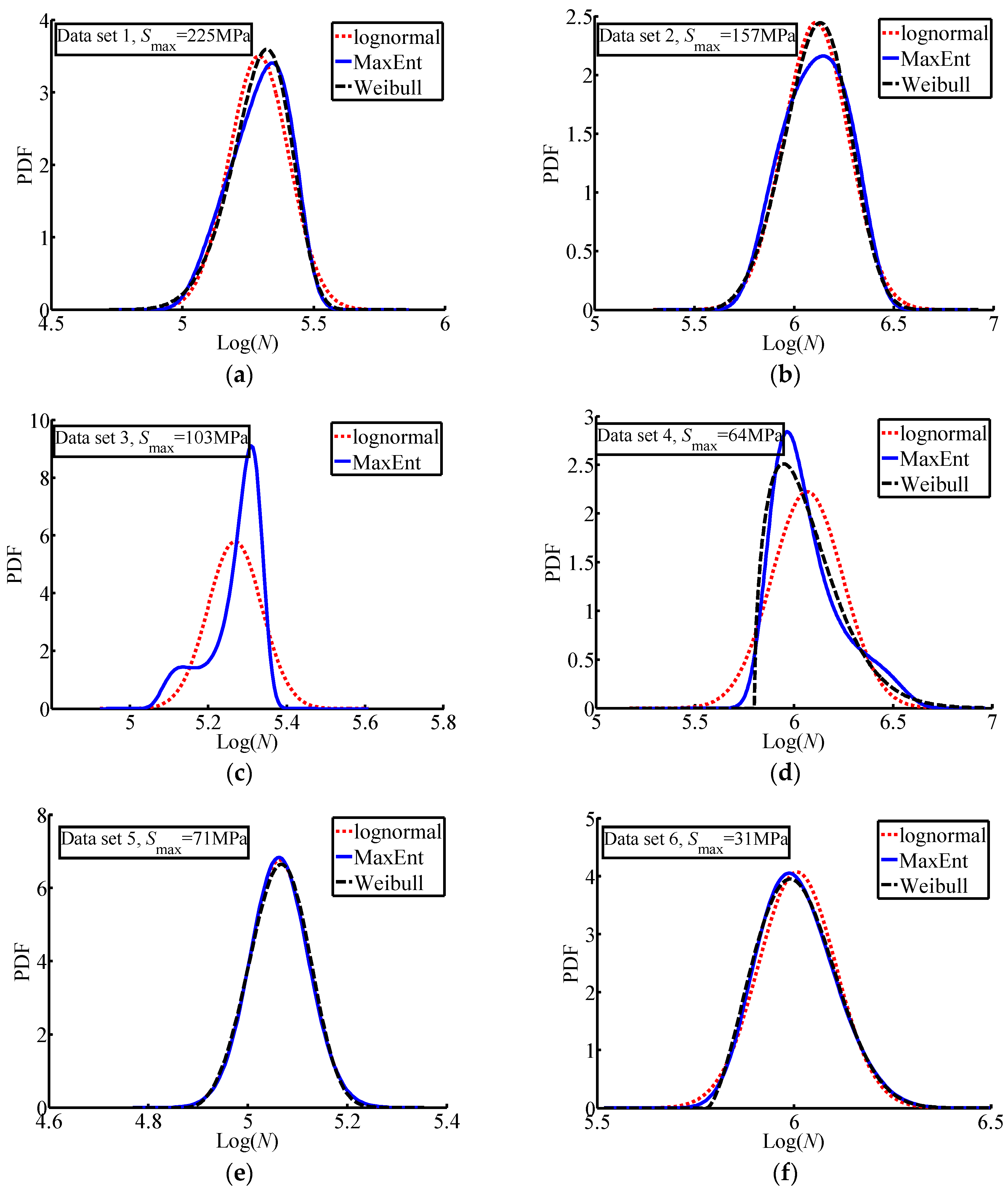
5.1. Six Fatigue Data Sets From Schijve’s Study

The presented MaxEnt distribution, the log-normal distribution and the three-parameter Weibull distribution are firstly applied to six fatigue data sets of 18 to 30 similar fatigue tests in Schijve’s work [4]. The experimental information is summarized in

Table 1. Experimental information of six fatigue data sets.

Specimen	Data Set	Thickness (mm)	Stress (MPa)		Number of Specimens
Unnotched Kt =1.15		2.0	Smax (R = 0)
	1		225		20
	2		157		18
Edge notched Kt =2.85		5.0	Smax (R = 0)
	3		103		20
	4		64		30
Riveted lap joint		0.8	Sm	Sa
	5		88	71	20
	6		88	31	20

. Three kinds of specimens were involved in this fatigue testing, i.e., unnotched, edge notched and riveted lap joint. In addition, two stress levels were considered. In order to apply the presented MaxEnt distribution, we first calculated the first four statistical moments of fatigue lives, as shown in

Table 2. Statistical moments of six fatigue data sets.

Data Set	Mean	SD	Skewness	Kurtosis
1	5.2921	0.1140	−0.3491	2.5835
2	6.1107	0.1632	−0.0985	2.3992
3	5.2680	0.0690	−1.0909	3.4517
4	6.0676	0.1795	0.8843	3.3241
5	5.0636	0.0589	0.0320	3.0828
6	6.0081	0.0980	0.3066	2.9434

. For the original test results, please refer to Schijve’s work [4].

The estimators of all parameters in three distributions are listed in

Table 3. Estimators of parameters in three probability distributions.

Data Set	Lognormal		Weibul1l			MaxEnt Distribution
	${\mu }_{\log \left(N\right)}$	${\sigma }_{\log \left(N\right)}$	$\alpha$	$\beta$	$\log (N_0)$	${\lambda }_0$	${\lambda }_1$	${\lambda }_2$	${\lambda }_3$	${\lambda }_4$
1	5.2921	0.1140	0.7082	6.8412	4.6301	−1.1427	0.3288	−0.2507	−0.1386	−0.0623
2	6.1107	0.1632	0.6799	4.3882	5.4911	−0.7592	0.0966	−0.2011	−0.0405	−0.0635
3	5.2680	0.0690	-	-	-	−1.6724	1.4226	−0.3391	−0.7755	−0.2071
4	6.0676	0.1795	0.2978	1.5187	5.8004	−0.7451	−0.8848	−0.3598	0.4182	−0.1045
5	5.0636	0.0589	0.2186	3.8061	4.8660	−1.9222	−0.0145	−0.5187	0.0047	0.0030
6	6.0081	0.0980	0.2575	2.5214	5.7800	−1.3785	−0.1945	−0.4412	0.0712	−0.0156

. Unfortunately, no Weibull distribution could be filled to data set 3 through the least square method. The computational results of fit indexes are listed in

Table 4. Fit indexes of three investigated probability distributions.

Data Set	Lognormal			Weibull			MaxEnt
	r.m.s.	d1	d2	r.m.s.	d1	d2	r.m.s.	d1	d2
1	0.0187	0.0112	0.0227	0.0149	0.0011	0.0102	0.0163	0.0067	0.0060
2	0.0335	−0.0022	0.0285	0.0325	−0.0048	0.0247	0.0337	−0.0003	0.0239
3	0.0242	0.0208	0.0143	-	-	-	0.0122	0.0102	−0.0373
4	0.0459	−0.0639	−0.0438	0.0193	0.0053	0.0188	0.0159	−0.0106	0.0095
5	0.0092	0.0078	−0.0107	0.0097	0.0097	−0.0135	0.0090	0.0081	−0.0093
6	0.0135	0.0000	−0.0371	0.0127	0.0181	−0.0330	0.0117	0.0111	−0.03113

. In addition, Figure 1 and Figure 2 show the PDF curves and probability plots of these six fatigue data set.

From Table 4, it can be seen that the r.m.s. of the Weibull distribution are similar or smaller than those of the log-normal distribution. It implies that the Weibull distribution has a better total fit effect than the log-normal distribution for the investigated data sets. Comparing the r.m.s. of the presented MaxEnt distribution and the log-normal distribution, a similar conclusion can be drawn from Table 4, i.e., the MaxEnt distribution gives a better total fit effect than the log-normal distribution on the average. For data set 2, the r.m.s. values is 0.0335 for the log-normal distribution, and 0.0337 for the MaxEnt distribution. In fact, these two values are too small and close to be distinguished. Then, the r.m.s. of the Weibull distribution and the MaxEnt distribution are compared. In 4 of 6 data sets, the MaxEnt distribution has a smaller value of the r.m.s. than the Weibull distribution. It should be pointed out that the MaxEnt distribution is suited for the fatigue data set 4, with a good fit (the r.m.s. is 0.0122), while the Weibull distribution cannot provide a fit. For data set 4, the MaxEnt distribution and the Weibull distribution are also hardly to be distinguished since they have small values for the r.m.s of deviation. The above observations indicate that, on the average, the MaxEnt distribution is better than the Weibull distribution for the investigated fatigue data sets.

In the following subsection, we are going to make comparisons of the tail fit effects. For the log-normal distribution, data sets 1, 2 and 4 have the same trends, i.e., $d_1<d_2$, and data 3, 5 and 6 have the same trends, i.e., $d_1>d_2$. The trend of $d_1<d_2$ is preferred in engineering design because the predicted fatigue life may be conservative for the investigated fatigue data sets. 2 of 6 data sets i.e., sets 2 and 4 show $d_1<0$, while the rest data sets have $d_1\ge 0$. For the Weibull distribution, data sets 1, 2 and 4 also show a trend of $d_1<d_2$, and data sets 5 and 6 have a trend of $d_1>d_2$. Based on this observation, it seems that the three-parameter Weibull distribution and log-normal distribution have the same predicted trend. For the MaxEnt distribution，data sets 2 and 4 have a trend of $d_1<d_2$, and the rest data set have a trend of $d_1>d_2$. However, the value of $d_1$ is very close to the $d_2$ in data set 1, which has been observed with a preferred trend of $d_1<d_2$. General speaking, those three distributions have similar predicted trend for the investigated fatigue data sets. In the next step, the number of data set with negative $d_1$ is checked for each probability distribution. Both the log-normal distribution and the MaxEnt distribution have 2 cases of $d_1<0$, i.e., data sets 2 and 4, while the Weibull distribution has only one cases of $d_1<0$, i.e., data sets 2. Considering these two parameters, all three probability distributions may give a non-conservative prediction in the tail region for the current investigated fatigue data.

The PDF curves of three distributions are shown in Figure 1. For data sets 1, 2, 5 and 6, the PDF shape obtained by three distributions are very similar to each other. This further confirms the observation from the comparison of r.m.s. in Table 4. Because the smallest differences among the r.m.s. are observed in Table 4, the smallest differences among the PDF curves of the three distributions can also be found in Figure 1e. As mentioned before, the three-parameter Weibull distribution is not suitable for data set 3. Both the log-normal distribution and the MaxEnt distribution can be used to fit data set 3. However, a bi-modal PDF is observed for the MaxEnt distribution. Investigating the r.m.s. values in Table 4, the MaxEnt distribution is better than the log-normal distribution for data set 3. For data set 4, the MaxEnt distribution is similar to the three-parameter Weibull, but different from the log-normal distribution (Figure 1d).

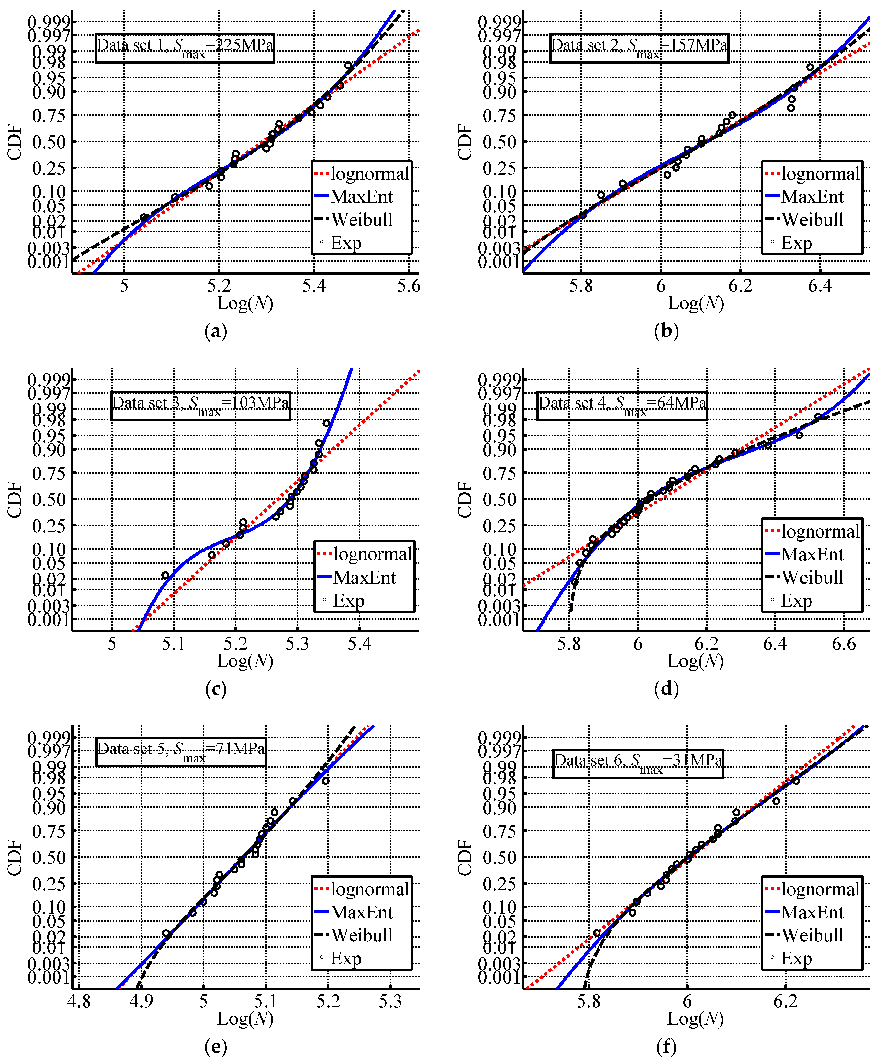
The probability plots of three distributions are given in Figure 2. For comparison purposes, the experimental data are plotted in Figure 2. These probability plots are obtained on a normal probability graph. This means the fitted normal distribution is a straight line, while the other two distributions are nonlinear curves. For data sets 1, 2, 5 and 6, the CDF curves obtained by the MaxEnt distribution and the Weibull distribution have good agreement with each other, especially for the region where experimental samples are available, and are better than those of the lognormal distribution. On the contrary, the difference among CDF curves is becoming bigger in the small probability region (left tail region on a PDF curve) and high reliability region (right tail region on a PDF curve). This phenomenon is not surprising since both the small probability region and high reliability region are generalized from the experimental data. From Figure 2c, it can be seen that data set 3 has an irregular trend. Although the lognormal distribution may be used to fit this data set, it is clear that the lognormal distribution disagrees with the trend of data. Integrating the information in Figure 2c, the MaxEnt distribution is the only proper distribution to fit data set 3, which has an irregular trend. For data set 4, the experimental data shows a similar trend as data set 3 because the specimens are the same just with different stress levels. All three investigated distributions may be used to fit it. However, Figure 2d further confirms the fact that both the MaxEnt distribution and the Weibull distribution are better than the lognormal distribution.

5.2. A Fatigue Data Set of Fatigue Crack Propagation

The experimental data of fatigue crack propagations [9] is selected to further demonstrate the performance of the presented MaxEnt distribution. The experimental system comprises an MTS dynamic testing machine, a machine controller, a LabVIEW signal generating/data acquisition system and a zoom microscope for the measurement of crack length. The metal material is 2024-T351 aluminum alloy, which is a major metal material in the aeronautical industry. The dimensions of the specimens were 50.0 mm wide and 12.0 mm thick. The nominal yield strength of the material is 320 MPa, the ultimate strength is 462 MPa, and the elongation is 15.4%.

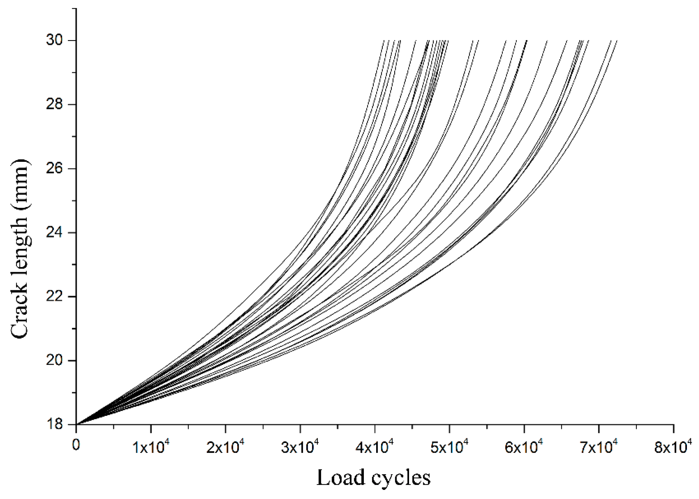
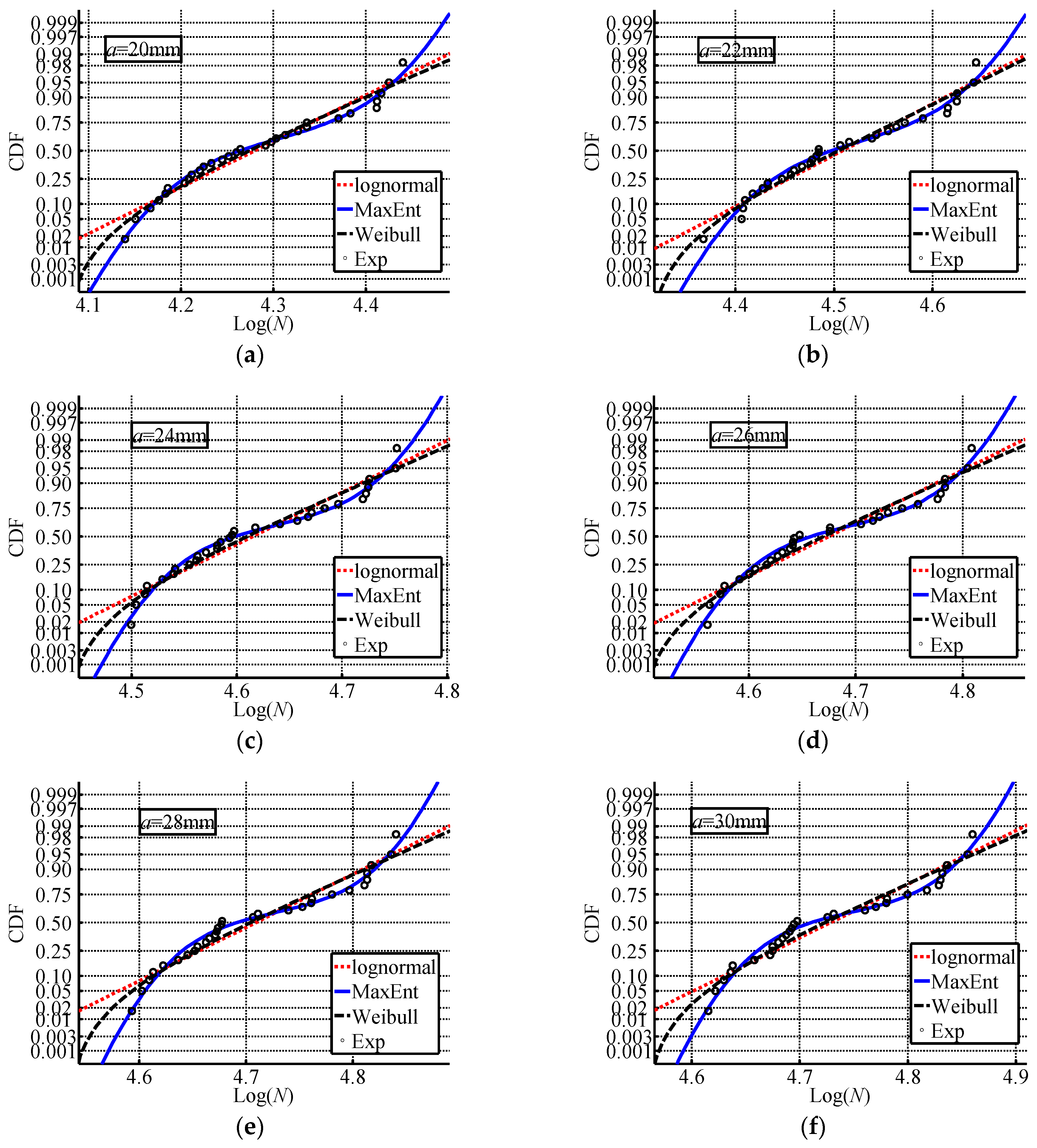
The crack length is started at a pre-cracking of 15.0 mm and extended to the length of 18.0 mm. During both the pre-cracking and fatigue crack growth tests, sinusoidal signals with maximum of 4.5 kN, minimum of 0.9 kN, and frequency of 15 Hz were used as the input loads. Figure 3 shows the crack propagation curves for all 30 specimens. According to Equations (18)–(21), the statistical moments of fatigue lives at different crack lengths are summarized in

Table 5. The statistical moments of fatigue lives at different crack lengths.

Length (mm)	Mean	SD	Skewness	Kurtosis
20	4.2796	0.0899	0.2884	1.9006
22	4.5084	0.0807	0.2222	1.8750
24	4.6152	0.0797	0.2899	1.7897
26	4.6747	0.0783	0.2766	1.7638
28	4.7090	0.0778	0.2753	1.7266
30	4.7285	0.0772	0.2840	1.7295

.

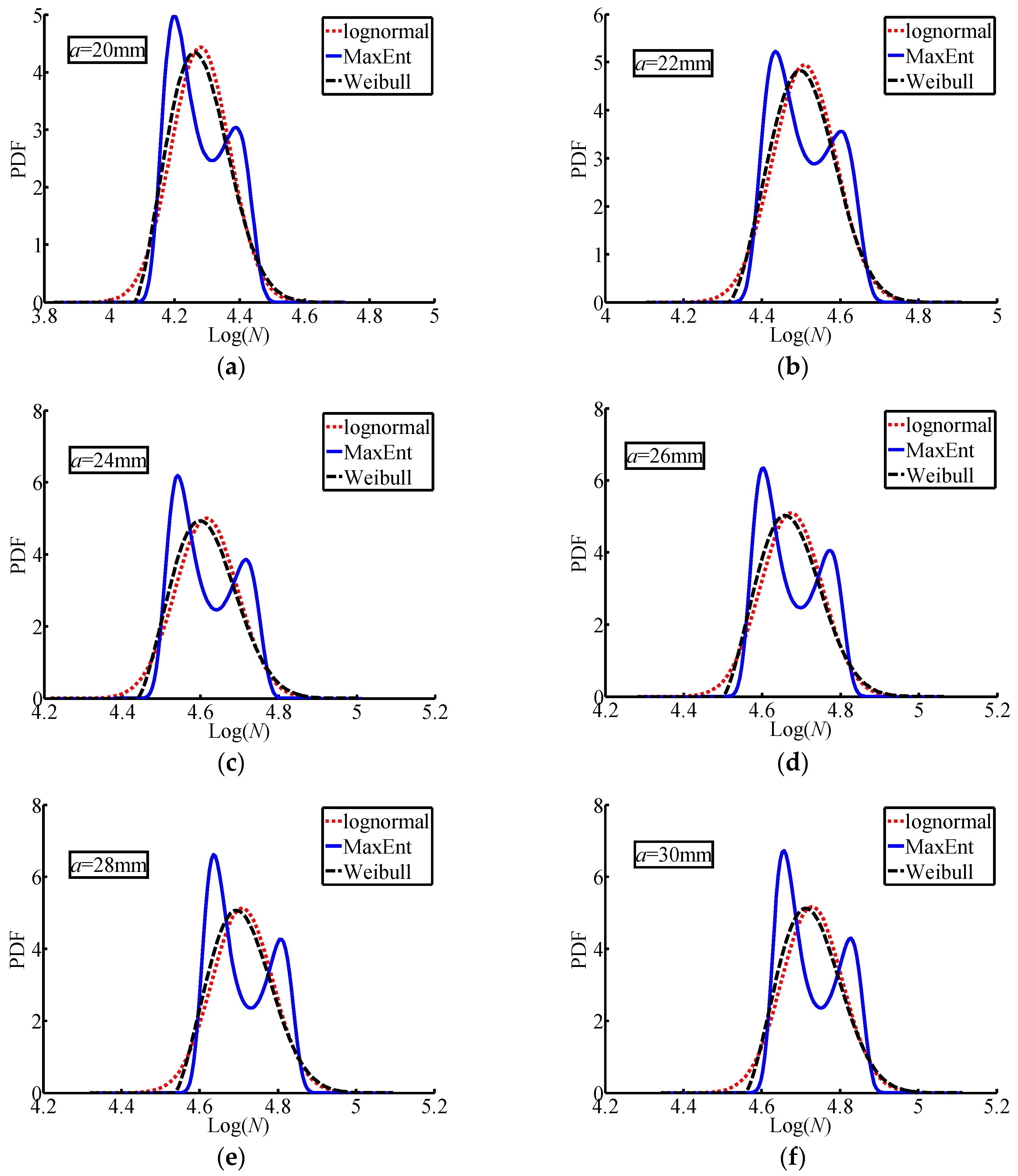
Based on the statistical moments in Table 5, the MaxEnt principle was applied to identify the probability distributions under different crack lengths, i.e., a = 22, 24, 26, 28 and 30 mm.

Table 6. Estimators of parameters in three probability distributions at different crack lengths.

Length (mm)	Lognormal		Weibull			MaxEnt Distribution
	${\mu }_{\log \left(N\right)}$	${\sigma }_{\log \left(N\right)}$	$\alpha$	$\beta$	$\log (N_0)$	${\lambda }_0$	${\lambda }_1$	${\lambda }_2$	${\lambda }_3$	${\lambda }_4$
20	4.2796	0.0899	0.2290	2.4495	4.0768	−1.0173	−0.5796	0.6485	0.3236	−0.3390
22	4.5084	0.0807	0.2205	2.6682	4.3126	−1.1289	−0.4404	0.6408	0.2433	−0.3258
24	4.6152	0.0797	0.1989	2.4115	4.4391	−1.0106	−0.6870	0.9801	0.4080	−0.4631
26	4.6747	0.0783	0.1972	2.4424	4.5001	−1.0030	−0.6743	1.0491	0.4043	−0.4867
28	4.7090	0.0778	0.1969	2.4616	4.5347	−0.9555	−0.7113	1.1876	0.4356	−0.5408
30	4.7285	0.0772	0.1923	2.4220	4.5582	−0.9618	−0.7362	1.1917	0.4516	−0.5447

gives the estimators of parameters in three distributions at different crack lengths.

Table 7. Fit indexes of three probability distributions at different crack lengths.

Length (mm)	Lognormal			Weibull			MaxEnt
	r.m.s.	d1	d2	r.m.s.	d1	d2	r.m.s.	d1	d2
20	0.0188	−0.0435	−0.0262	0.0154	−0.0250	−0.0111	0.0075	−0.0019	0.0118
22	0.0171	−0.0241	−0.0519	0.0151	−0.0079	−0.0458	0.0082	0.0102	−0.0388
24	0.0193	−0.0569	−0.0327	0.0163	−0.0386	−0.0165	0.0073	−0.0097	0.0111
26	0.0203	−0.0572	−0.0275	0.0165	−0.0395	−0.0106	0.0074	−0.0099	0.0186
28	0.0200	−0.0511	−0.0362	0.0175	−0.0318	−0.0208	0.0078	−0.0003	0.0090
30	0.0203	−0.0549	−0.0328	0.0177	−0.0351	−0.0154	0.0081	−0.0036	0.0153

summarizes the fit indexes of the three distributions. It is found that the expressions of PDFs for fatigue lives at different crack length are very similar to each other if only one of three distributions is considered. Comparing the r.m.s of deviations (Table 7), the presented MaxEnt distribution produced the smallest values among three distributions for all crack lengths, and the three-parameter Weibull distribution yields smaller values than the lognormal distribution for all crack lengths. In other words, regarding the total fit effects, the MaxEnt distribution is the best choice for this fatigue data set. For all three distributions, five out of six crack lengths show a trend of $d_1<d_2$, except at a = 22 mm, which indicates conservative evaluations in the left tails. In addition, most of $d_1$ have negative values, except for a = 22 mm from the MaxEnt distribution.

The PDF curves and probability plots for three distributions are plotted in Figure 4 and Figure 5, respectively. It is obvious that the identified distributions by the MaxEnt principle are not the commonly used standard distribution type. Taking a close look at the identified PDF curves, bimodal PDFs are observed from the MaxEnt principle in this case study (Figure 4). They are very different for standard probability distributions, e.g., the lognormal distribution and the Weibull distribution in this study. From Figure 5, it can be seen that all fatigue lives have an irregular trend like in data set 3 in test example 1. The MaxEnt distribution shows a better agreement with the experimental data than that of the lognormal distribution and the Weibull distribution. Using the same experimental data, both the lognormal and Weibull distribution can pass hypothesis testing. However, the CDFs of fatigue lives identified by the lognormal and Weibull distribution cannot match the experimental data well. This indicates that the commonly used standard probability distributions are not suitable to descript the scatter in fatigue lives in this case study.

For comparison purposes, the computational results reported by Wu and Ni [9] should be also considered in this study. It should be pointed out that Wu and Ni adopted a stochastic process method [7,26] which seems to have an advanced mathematical theory, however, the computational results are almost the same to the lognormal distribution. Compared with the experimental data, the MaxEnt distribution is better than the stochastic process method. Furthermore, the implementation procedure of the proposed method is much easier than that of the stochastic process method.

6. Conclusions

A new computational method is proposed in this paper for identifying the probability distribution of fatigue life of materials and structures. It is based on the first four statistical moments of fatigue life and the maximum entropy principle. The first four statistical moments are calculated from samples of fatigue life in a fatigue testing or measurement. Then, they serve as constraints in the maximum entropy principle. The corresponding optimization problem in the maximum entropy principle is solved by transferring it into an unconstrained optimization problem using a potential function. This strategy avoids the possible numerical singularity when solving N nonlinear equations. The following conclusions have been reached:

(1)

The MaxEnt distribution is the most natural distribution given the fatigue life samples. It reduces the introduction of subjective uncertainty when a standard distribution is chosen to model fatigue life. Additionally, the presented method has many significant characteristics, such as simply concept, high efficiency, easy programming, wide applicability, etc.

(2)

A careful comparison between the MaxEnt distribution, the lognormal distribution and the three-parameter distribution has been carried out in this paper. The three-parameter Weibull distribution has a minimum of fatigue life (N₀) as the third parameter. This seems to be consistent with fatigue physics, but the physical significance of this minimum fatigue life remains unclear because its estimated value is obtained by an iteration algorithm without any physical concepts. Due to the existing of the third parameter, the three-parameter Weibull distribution cannot be performed in extremely cases, e.g., data set 3 in test example 1.

(3)

The fatigue life distributions of two groups of fatigue data sets were identified by the lognormal distribution, the Weibull distribution and the MaxEnt distribution. The computational results show that both the Weibull distribution and the MaxEnt distribution have a better agreement with the experimental data than the lognormal distribution. The most attractive feature is that the MaxEnt distribution is better than the Weibull distribution on average, especially for the cases where the fatigue life CDF has an irregular trend.