An Estimator of Mutual Information and its Application to Independence Testing

Abstract

This paper proposes a novel estimator of mutual information for discrete and continuous variables. The main feature of this estimator is that it is zero for a large sample size n if and only if the two variables are independent. The estimator can be used to construct several histograms, compute estimations of mutual information, and choose the maximum value. We prove that the number of histograms constructed has an upper bound of $O(\log n)$ and apply this fact to the search. We compare the performance of the proposed estimator with an estimator of the Hilbert-Schmidt independence criterion (HSIC), though the proposed method is based on the minimum description length (MDL) principle and the HSIC provides a statistical test. The proposed method completes the estimation in $O(n\log n)$ time, whereas the HSIC kernel computation requires $O(n^3)$ time. We also present examples in which the HSIC fails to detect independence but the proposed method successfully detects it.

1. Introduction

Shannon’s information theory [1] has contributed to the development of communication and storage systems in which sequences can be compressed up to the entropy of the source assuming that the sender and receiver know the probability of each sequence. In the 30 years since its birth, information theory has developed such that sequences can be compressed without sharing the associated probability (universal coding): the probability of each future sequence can be learned from the past sequence such that the compression ratio of the total sequence converges to its entropy.

Mutual information is a quantity that can be used to analyze the performances of encoding and decoding in information theory, and its value expresses the dependency of two random variables and is nonnegative (that is, zero) if and only if they are independent. Mutual information can be estimated from actual sequences. In this paper, we construct an estimator of the mutual information based on the minimum description length (MDL) principle [2] such that the estimator is zero if and only if the two variables are independent for long sequences.

In any science, a law is determined based on experiments: the law should be simple and explain the experiments. Suppose that we generate pairs of a rule and its exceptions for the experiments and describe the pairs using universal coding. Then, the MDL principle chooses the rule of the pair that has the shortest description length (the number of bits) as the scientific law: the simpler the rule is, the more exceptions there are. In our situation, two variables may be either independent or dependent, and we compute the values of the corresponding description lengths to choose one of them based on which length is shorter. We estimate mutual information based on the difference between the description length values assuming that the two variables are independent and dependent, divided by the original sequence length n.

Let X and Y be discrete random variables. Suppose that we have examples $(X=x_1,Y=y_1),\cdots ,$ $(X=x_n,Y=y_n)$ and that we wish to know whether X and Y are independent, denoted as $X\perp \perp Y$, not knowing the distributions $P_X,P_Y$, and $P_{XY}$ of X, Y and $(X,Y)$, respectively.

One way of approaching this problem would be to estimate the correlation coefficient $\rho (X,Y)$ of $X,Y$ to determine whether it is close to zero. Although the notions of independence and correlation are close, simply because $\rho (X,Y)=0$ does not mean that X and Y are independent. For example, let X and U be mutually independent variables with a standard Gaussian distribution and $\{-1,1\}$ with probability 0.5, respectively, and let $Y=XU$. Apparently, X and Y are not independent, but note that $EX=EY=0$, $VX=E{X}^2=1$, $VY=E\left[U^2{X}^2\right]=E{X}^2=1$, and

$$cov(X,Y)=E\left[XY\right]=E\left[X^{2}U\right]=0.5·E{X}^2+0.5·E[-X^2]=0,$$

which means that $\rho (X,Y)=cov(X,Y)/\sqrt{VX·VY}=0.$

For this problem, we know that the mutual information defined by

$$I(X,Y):=\sum _x\sum _y{P}_{XY}(x,y)\log \frac{P_{XY}(x,y)}{P_X(x)P_Y(y)}$$

satisfies

$$I(X,Y)=0⟺X\perp \perp Y.$$

Thus, it is sufficient to estimate $I(X,Y)$ to determine whether it is positive.

Given $x^n=(x_1,\cdots ,x_n)$ and $y^n=(y_1,\cdots ,y_n)$, one might estimate $I(X,Y)$ by plugging in the frequencies $c_X(x)$, $c_Y(y)$, and $c_{XY}(x,y)$ of $X=x$, $Y=y$, and $(X,Y)=(x,y)$ divided by n into $P_X$, $P_Y$, and $P_{XY}$, respectively, to obtain the quantity

$$I_n:=\sum _x\sum _y\frac{c_{XY}(x,y)}{n}\log \frac{{\displaystyle \frac{c_{XY}(x,y)}{n}}}{{\displaystyle \frac{c_X(x)}{n}\frac{c_Y(y)}{n}}}.$$

(1)

However, we observe that $I_n>0$ even when $X\perp \perp Y$ for large values of n. In fact, since Equation (1) is the Kullback-Leibler divergence between $\frac{c_{XY}(x,y)}{n}$ and $\frac{c_X(x)}{n}·\frac{c_Y(x)}{n}$, we have $I_n\ge 0$, and $I_n=0$ if and only if

$$\frac{c_{XY}(x,y)}{n}=\frac{c_X(x)}{n}·\frac{c_Y(x)}{n}$$

for all $x,y$, which does not hold infinitely many times with a positive probability, even when $X\perp \perp Y$. Thus, we need to guess $X\perp \perp Y$ when $I_n$ is small, say when $I_n<\delta (n)$ for some appropriate function of n:

$$I_n\le \delta (n)⟺X\perp \perp Y.$$

(2)

Nobody was certain that such a function $\delta (n)$ of sample size n exists.

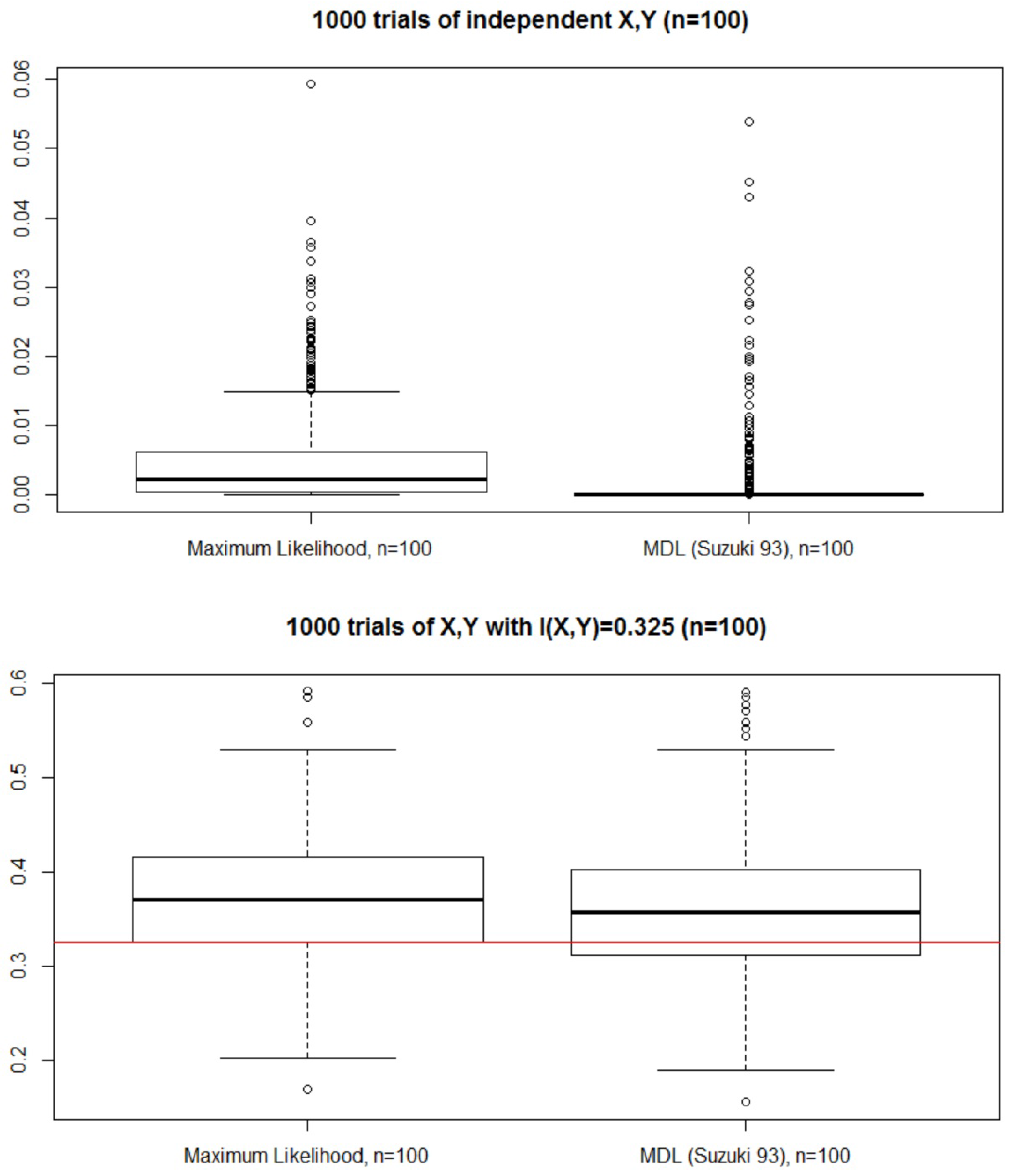
In 1993, Suzuki [3] identified such a function δ and proposed a new mutual information estimator $J_n:=I_n-\delta (n)$ such that

$$J_n\le 0⟺X\perp \perp Y$$

(3)

for large n based on the minimum description length (MDL) principle. The exact form of function δ is presented in Section 2. In this paper, we consider an extension of the estimation $J_n$ of mutual information $I(X,Y)$ for a case where X and Y may be continuous.

There are many ways of estimating mutual information for continuous variables. If we assume that X and Y are Gaussian, then the mutual information is expressed by

$$I(X,Y)=-\frac{1}{2}\log \{1-\rho {(X,Y)}^2\}$$

and we can show that

$$I_n-\frac{1}{2n}\log n\le 0⟺X\perp \perp Y$$

(4)

for large n, where $I_n$ is the maximum likelihood estimator of $I(X,Y)$. However, the equivalence only holds for Gaussian variables.

For general settings, several mutual information estimators are available, such as kernel density-based estimators [4], k-nearest neighbors [5,6], and other estimators based on quantizers [7]. In general, the kernel-based method requires an extraordinarily large computational effort to test for independence. To overcome this problem, efficient estimators have been proposed, such as one that completes the test in $O(n\log n)$ time [5]. However, correctness, such as consistency, is required and has a higher priority than efficiency. Although some of these methods converge to the correct value $I(X,Y)$ for large n in $O(n\log n)$ time [7], the estimation values are positive with nonzero probability for large n when X and Y are independent ($I(X,Y)=0$).

Currently, the construction of nonlinear alternatives of $cov(X,Y)$ to test for independence between X and Y by using positive definite kernels is becoming popular. In particular, a quantity known as the Hilbelt-Schmidt independence criterion (HSIC) [8], which is defined in Section 2, is extensively used for independence testing. It is known that the HSIC value $HSIC(X,Y,k,l)$ depends on the kernels k and l w.r.t. the ranges of X and Y, and

$$HSIC(X,Y,k,l)=0⟺X\perp \perp Y$$

(5)

if the kernel pair $(k,l)$ is chosen properly. In this paper, we assume that we always use such a kernel pair and denote $HSIC(X,Y,k,l)$ simply by $H(X,Y)$. For the estimation of $H(X,Y)$ given $x^n$ and $y^n$, the most popular estimator $H_n$ of $H(X,Y)$, which is defined in Section 2, always takes positive values, and given a significance level of $0<\alpha <1$ (typically, $\alpha =0.05$), we need to obtain $ϵ(\alpha )$ such that the decision

$$H_n<ϵ(\alpha )⟺X\perp \perp Y$$

is as accurate as possible.

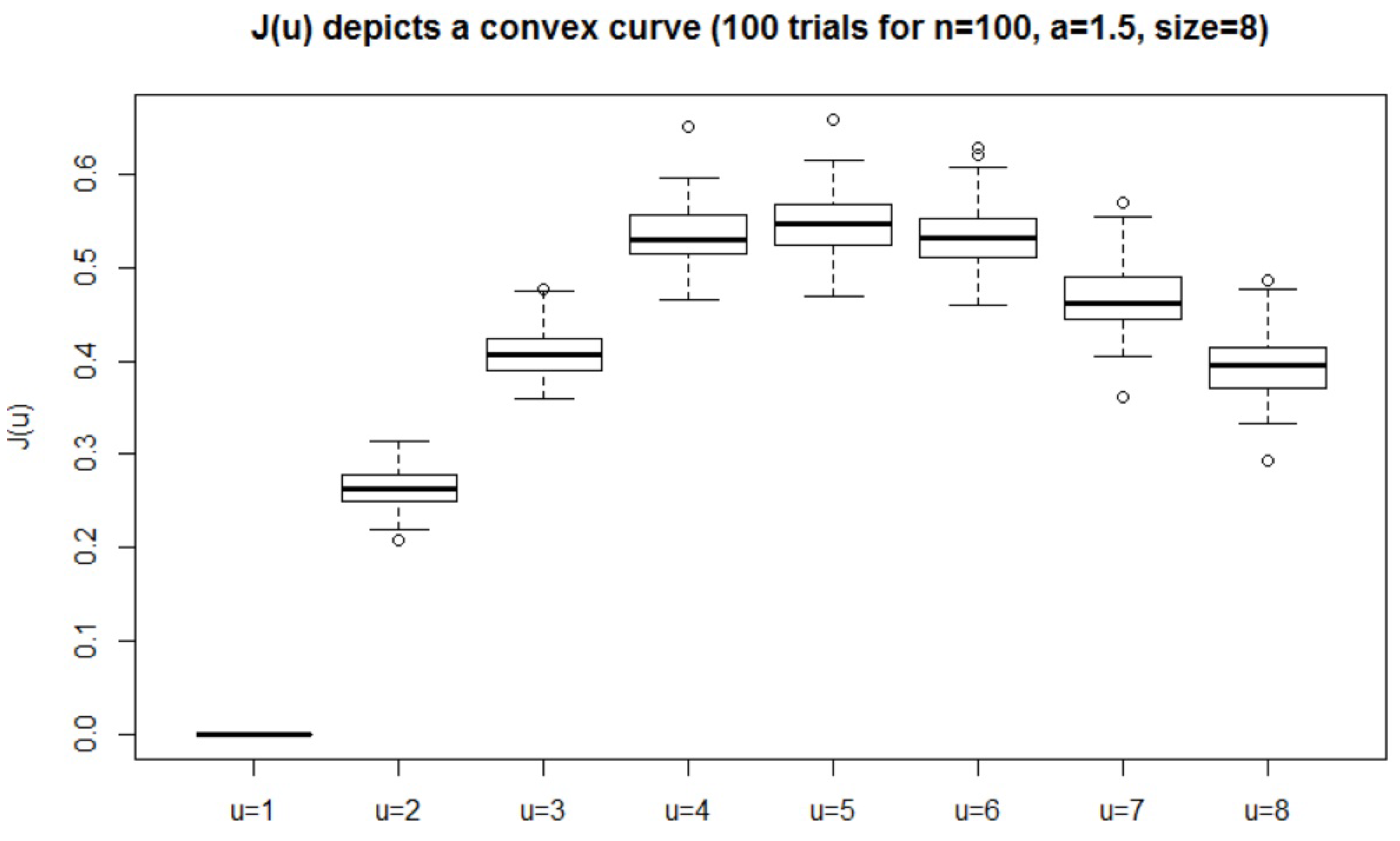
In this paper, we propose a new estimator $J_n$ of mutual information. This new estimator quantizes the two-dimensional Euclidean space ${\mathbb{R}}^2$ of X and Y into $2^u\times 2^u$ bins for $u=1,2\cdots$. For each value of u that indicates a histogram, we obtain the estimation $J_n^{(u)}$ of mutual information for discrete variables. The maximum value of $J_n^{(u)}$ over $u=1,2,\cdots$ is the final estimation. We prove that the optimal value of u is at most $O(\log n)$. In particular, the proposed method divides ${\mathbb{R}}^2$ without distinguishing between discrete and continuous data, and it satisfies Equation (3).

Then, we experimentally compare the proposed estimator $J_n$ of $I(X,Y)$ with the estimator $H_n$ of HSIC $H(X,Y)$ in terms of independence testing. Although we obtained several insights, we could not obtain confirmation that one of the estimators outperforms the other. However, we found that the HSIC only considers the magnitude of the data and would fail to detect relations among the data that cannot be identified by simply observing the changes in magnitude. We present two examples for which the HSIC fails to detect the dependencies among $x^n$ and $y^n$ due to the aforementioned limitation. The proposed estimation procedure completes the computation in $O(n\log n)$ time, whereas the HSIC requires $O(n^3)$ time. In this sense, the proposed method based on mutual information would be useful in many situations.

The remainder of this paper is organized as follows. Section 2 provides the background for the work presented in this paper, and Section 2.1 and Section 2.2 explain the mutual information and HSIC estimations, respectively. Section 3 presents the contributions of this paper, and Section 3.1 proposes the new algorithm for estimating mutual information. Section 3.2 mathematically proves the merits of the proposed method, and Section 3.3 presents the results of the preliminary experiments. Section 4 presents the results of the experiments using the R language to compare the performance in terms of independence testing for the proposed estimator of mutual information and its HSIC counterpart. Section 5 summarizes the contributions and discusses opportunities for future work.

Throughout the paper, the base two logarithm is assumed unless specified otherwise.

2. Background

This section describes the basic properties of the estimations of mutual information $I(X,Y)$ for discrete variables and HSIC $H(X,Y)$.

2.1. Mutual Information for Discrete Variables

In 1993, Suzuki [3] proposed an estimator of mutual information based on the minimum description length (MDL) principle [2]. Given examples, the MDL chooses a rule that minimizes the total description length when the examples are described in terms of a rule and its exceptions. In this case, there are two candidate rules: X and Y are either independent or not. When they are independent, for each X and Y, we first describe the independent conditional probability values, and using them, the examples can be described. The total length will be

$$L^n(x^n):=-\sum _x{c}_X(x)\log \frac{c_X(x)}{n}+\frac{\alpha -1}{2}\log n$$

(6)

plus

$$L^n(y^n):=-\sum _y{c}_Y(y)\log \frac{c_Y(y)}{n}+\frac{\beta -1}{2}\log n$$

(7)

up to constant values, where α and β are the cardinalities of X and Y, respectively. When they are not independent, we describe the examples in length

$$L^n(x^n,y^n):=-\sum _x\sum _y{c}_{XY}(x,y)\log \frac{c_{XY}(x,y)}{n}+\frac{\alpha \beta -1}{2}\log n$$

(8)

up to constant values. Hence, the difference Equation (6) + Equation (7) − Equation (8) divided by n is

$$J_n=I_n-\frac{(\alpha -1)(\beta -1)}{2n}\log n.$$

(9)

It is known that

$$J_n\le 0⟺X\perp \perp Y$$

(10)

for large n [9], which means that ${\displaystyle \delta (n)=\frac{(\alpha -1)(\beta -1)}{2n}\log n}$ in Equation (2). Figure 1 presents a box plot of 1000 trials for the two estimations for $n=100$ and $\alpha =\beta =2$, where X and Y are independent and dependent, respectively.

Figure 1. Estimating mutual information: the minimum description length (MDL) computes the correct values, whereas the maximum likelihood yields values that are larger than the correct values.

Although the estimator of mutual information is defined by Equation (9) in the original paper by Suzuki [3], in this paper, we define

$$J_n:=max\{I_n-\frac{(\alpha -1)(\beta -1)}{2n}\log n,0\}$$

instead such that Equation (10) is replaced by

$$J_n=0⟺X\perp \perp Y.$$

2.2. Maximizing the Posterior Probability

Note that this paper seeks whether $X\perp \perp Y$ or not rather than the mutual information value itself.

We claim that the decision (9.5) asymptotically maximizes the posterior probability of $X\perp \perp Y$ given $x^n$ and $y^n$. Let $Q^n(X):=\int {\prod }_x{\theta }_x^{n_x}w(\theta |a)d\theta$, where $n_x$ is the occurrence of $X=x$ in $x^n$, and $w(\theta |a)\propto {\prod }_x{\theta }_x^{a_x-1}$ is the prior probability of the probability $\theta =({\theta }_x)$ of $X=x$ assuming the hyper-parameters $a=(a_x)$ with $a_x>0$. Suppose that we similarly construct $Q^n(Y)$ and $Q^n(X,Y)$ with $a_y>0$ and $a_{xy}>0$. It is known that if we choose $a_x=0.5$, $a_y=0.5$, and $a_{xy}=0.5$, then $L^n(x^n)+\log Q^n(X)$, $L^n(y^n)+\log Q^n(Y)$, and $L^n(x^n,y^n)+\log Q^n(X,Y)$ are bounded by constants [10]. Hence, for large n, we have

$$p{Q}^n(X)Q^n(Y)\ge (1-p)Q^n(X,Y)⟺J_n=0,$$

where the prior probability p of $X\perp \perp Y$ is a constant and is negligible for large n.

On the other hand, Nemenman, Shafee, and Bialek [11] proposed a Bayesian estimator

$$H^n(x^n,a):=\int (-\sum _x{\theta }_x\log {\theta }_x)w(\theta |x^n,a)d\theta$$

and its expectation $H^n(x^n)$ w.r.t. a prior over the hyper-parameter $a=(a_x)$, where ${\theta }_x$ is the probability of the event $(X=x)$. If we similarly construct a Bayesian estimators $H^n(y^n)$ and $H^n(x^n,y^n)$ of entropies $H(Y)$, $H(X,Y)$, respectively, then we also obtain a Bayesian estimator

$$I_{NSB}^n(x^n,y^n):=H^n(x^n)+H^n(y^n)-H^n(x^n,y^n)$$

of mutual information $I(X,Y)$ [12]. M. Hutter [13] proposed another estimator

$$I^n(x^n,y^n,a):=\int (\sum _x\sum _y{\theta }_{xy}\log \frac{{\theta }_{xy}}{{\theta }_x{\theta }_y})w(\theta |x^n,y^n,a)d\theta$$

(11)

and its expectation $I_H^n(x^n,y^n)$ w.r.t. a prior over the hyper-parameter $a=(a_x,a_y)$, where ${\theta }_y$ and ${\theta }_{xy}$ are the probabilities of the events $(Y=y)$ and $(X=x,Y=y)$.

The main drawback of estimators $I_{NSB}^n$ and $I_H^n$ is that both of

$$I_{NSB}^n(x^n,y^n)=0⟺X\perp \perp Y$$

$$I_H^n(x^n,y^n)=0⟺X\perp \perp Y$$

fail for large n. For example, we have $I^n(x^n,y^n,a)>0$ unless $w(\theta |x^n,y^n,a)$ concentrates on the case ${\theta }_{xy}={\theta }_x{\theta }_y$ for all $x,y$, which occurs with probability zero even when $X\perp \perp Y$. Note that they seek the mutual information value itself rather than whether $X\perp \perp Y$ or not.

2.3. HSIC

The HSIC is formally defined by

$$H(X,Y):=E_{X{X}^{\prime }Y{Y}^{\prime }}\left[k(X,X^{\prime })l(Y,Y^{\prime })\right]+E_{X{X}^{\prime }}\left[k(X,X^{\prime })\right]·E_{Y{Y}^{\prime }}\left[l(Y,Y^{\prime })\right]-2E_{XY}\{E_{X^{\prime }}\left[k(X,X^{\prime })\right]E_{Y^{\prime }}\left[l(Y,Y^{\prime })\right]\}$$

(12)

using the positive definite kernels $k:{\mathcal{X}}^2\to \mathbb{R}$ and $l:{\mathcal{Y}}^2\to \mathbb{R}$, where $\mathcal{X}$ and $\mathcal{Y}$ are the ranges of X and Y, respectively, and $P_{XY}=P_{X^{\prime }{Y}^{\prime }}$. The most common estimator of $H(X,Y)$, given $x^n$ and $y^n$, would be

$$\begin{array}{c}\hfill H_n:=\frac{1}{n^2}\sum _{i,j}k(x_i,x_j)l(y_i,y_j)+\frac{1}{n^4}\sum _{i,j}k(x_i,x_j)\sum _{p,q}l(y_p,y_q)-\frac{2}{n^3}\sum _{i,p.q}k(x_i,x_p)l(y_i,y_q)\}.\end{array}$$

(13)

We prepare $0<\alpha <1$ (for example, $\alpha =0.05$). Then, there exists a threshold $ϵ(\alpha )$ such that if the null hypothesis is true, then the value of $H_n$ should be less than $ϵ(\alpha )$ with probability $1-\alpha$. The decision is based on

$$H_n<ϵ(\alpha )⟺X\perp \perp Y.$$

Applying HSIC to independence testing is widely accepted in the machine learning community; in addition to the equivalence Equation (5) with independence, (weak) consistency has been shown in the sense that the difference between Equations (12) and (13) is at most $O(1/\sqrt{n})$ in probability [8]. Furthermore, HSIC exhibits satisfactory performance in actual situations and is currently considered to be the de facto method for independence testing.

However, we still encounter serious problems when applying HSIC. The most significant problem is that HSIC requires $O(n^3)$ computational time, and n is required to be small if it is necessary that the test be completed within a predetermined time. Moreover, the calculation of the correct value of $ϵ(n)$ requires many hours for simulating the null hypothesis. Given $x^n$ and $y^n$, we randomly reorder $y^n$ to obtain independent pairs of examples and compute $H_n$ many times to obtain the $(1-\alpha )\times 100$ percentile point $ϵ(\alpha )$. If $\alpha =0.05$, then we obtain 10 samples of a higher $\alpha \times 100$ percentile to ensure that the value of $ϵ(\alpha )$ is correct by executing the computation more than 200 times.

3. Estimation of Mutual Information for both Discrete and Continuous Variables

This paper proposes a new estimator of mutual information that is able to address both discrete and continuous variables and that becomes zero if and only if X and Y are independent for large n.

3.1. Proposed Algorithm

The proposed estimation consists of three steps:

• prepare nested histograms [14],
• compute estimations $J_n^{(u)}$ of mutual information for the histogram $s=1,2,\cdots$, and
• choose the maximum among the estimations $J_n^{(u)}$ w.r.t. the histograms $u=1,2,\cdots$.

Suppose that we are given examples $x^n=(x_1,\cdots ,x_n)$ and $y^n=(y_1,\cdots ,y_n)$ and that they have been sorted as

$${\tilde{x}}_1\le {\tilde{x}}_2\le \cdots \le {\tilde{x}}_n\mathrm{and}{\tilde{y}}_1\le {\tilde{y}}_2\le \cdots \le {\tilde{y}}_n.$$

(14)

First, we assume that no consecutive values are equal in each of the two sequences Equation (14), which is true with probability one when the density function exists. Let $s\ge 1$ be an integer, and for each $u=1,\cdots ,s$, we prepare histograms with $2^u$ bins for X, Y, and $(X,Y)$. Let $t:=n/2^u$. The sequences Equation (14) are divided into clusters such as

$$({\tilde{x}}_1,\cdots ,{\tilde{x}}_{\lfloor t\rfloor }),\cdots ({\tilde{x}}_{{}_{\lfloor (j-1)t\rfloor }+1},\cdots ,{\tilde{x}}_{\lfloor jt\rfloor }),\cdots ,({\tilde{x}}_{{}_{\lfloor (2^u-1)t\rfloor }+1},\cdots ,{\tilde{x}}_n)$$

and

$$({\tilde{y}}_1,\cdots ,{\tilde{y}}_{\lfloor t\rfloor }),\cdots ({\tilde{y}}_{{}_{\lfloor (k-1)t\rfloor }+1},\cdots ,{\tilde{y}}_{\lfloor kt\rfloor }),\cdots ,({\tilde{y}}_{{}_{\lfloor (2^u-1)t\rfloor }+1},\cdots ,{\tilde{y}}_n).$$

Thus, we have quantized sequences $x^n\mapsto a_u^n=(a_1^{(u)},\cdots ,a_n^{(u)})$ and $y^n\mapsto b_u^n=(b_1^{(u)},\cdots ,b_n^{(u)})$ with $u=1,\cdots ,s$ using the clusters. For example, suppose that we generate $n=1000$ standard Gaussian random sequences $x^n$ and $y^n$ with a correlation coefficient of $0.8$. The frequency distribution tables of $a^n$ and $b^n$ for $u=3$ are

  1   2   3   4   5   6   7   8

125 125 125 125 125 125 125 125

and that of $(a^n,b^n)$ for $u=3$ are as follows:

   1  2  3  4  5  6  7  8

1 75 32 12  5  1  0  0  0

2 25 41 25 18  9  7  0  0

3 15 23 32 27 14 11  1  2

4  5 17 24 22 27 19 11  0

5  5  9 19 24 23 23 17  5

6  0  3  7 18 26 26 28 17

7  0  0  6  9 19 21 45 25

8  0  0  0  2  6 18 23 76

Thus, the distributions of $a^n$ and $b^n$ are nearly uniform. Because a sufficient number of samples is allocated to each cluster, at least for one-dimensional $X,Y$ if n is large, the estimations are more robust than for other histogram-based methods [9].

Because the obtained sequences $a_u^n$ and $b_u^n$ are discrete, we can compute

$${\displaystyle J_n^{(u)}=I_n^{(u)}-\frac{K_n^{(u)}}{2n}\log n,}$$

(15)

where $I_n^{(u)}$ is the empirical mutual information w.r.t. histogram $u=1,2,\cdots$ and $K_n^{(u)}={(2^u-1)}^2$ is the number of independent parameters. The derivation of Equation (15) is similar to that of Equation (9).

Let $(X_u,Y_u)$ and $(X_v,Y_v)$ be the random variables for histograms u and v such that $u\le v$. Suppose that examples $a_v^n$ and $b_v^n$ have been emitted from $(X_v,Y_v)$; we wish to know whether $(X_v,Y_v)$ are conditionally independent given $(X_u,Y_u)$ based on the MDL principle. Then, we can answer the question affirmatively if we compare the description length values to find that $J_n^{(v)}\le J_n^{(u)}$. This means that according to the MDL principle, we can use the decision that $(X_v,Y_v)$ are conditionally independent given $(X_u,Y_u)$ if and only if $J_n^{(v)}\le J_n^{(u)}$. Hence, if u provides the maximum value of $J_n^{(u)}$, then we choose the histogram u. Thus, we propose the estimation given by ${\displaystyle J_n:=\underset{1\le u\le s}{max}{J}_n^{(u)}}$, and we prove why the optimal value of u is at most $s=\lfloor 0.5\log n\rfloor$ in Section 3.2 (Theorem 1).

Another interpretation is that if the sample size in each bin is smaller, then the estimation is less robust. However, if the number of bins is smaller, then the approximation of the histogram is less appropriate. These two factors are balanced by the MDL principle.

For example, suppose that $n=1000$; thus, $s=\lfloor 0.5\log 1000\rfloor =4$. If we have the following four values:

u    J(u)

1 0.2664842

2 0.5077115

3 0.5731657

4 0.4601272

then the final estimation will be 0.5731657 ($u=3$). Note that there are other methods for finding the maximum mutual information. For example, $s=\lfloor 0.5{\log }_{a}n\rfloor$ and $a^u$ clusters for each of $(X,Y)$ work if $a>1$ (the smaller a is, the larger s is). For $a=1.5$, we experimentally find (Figure 2) that the value of $J(u)$ depicts a concave curve, i.e., the maximum value is obtained at the point $u=5$ at which the sample size of each bin (robustness of the estimation) and the number of bins (approximation of the histogram) are balanced.

Figure 2. Values of $J_n^{(u)}$ with $1\le u\le s$: the maximum value is obtained at the point where the sample size of each bin and the number of bins are balanced.

Next, we consider the case for which two values at consecutive locations are the same in one of the two sequences Equation (14). In general, we divide each cluster in half at each stage $u=1,2,\cdots ,s$. If two values at consecutive locations are equal and they need to be divided, then we choose another border: suppose that k values are equal from the $(j+1)$-th location,

$${\tilde{x}}_j<{\tilde{x}}_{j+1}=\cdots ={\tilde{x}}_{j+k}<{\tilde{x}}_{j+k+1}.$$

and that we need to divide the $(j+i)$-th and $(j+i+1)$-th positions ($1\le i\le k-1$); rather, we either divide between the j-th and $(j+1)$-th positions or between the $(j+k)$-th and $(j+k+1)$-th positions, depending on whether $i<k/2$ or $i\ge k/2$. For example, if $n=8$ and $x^8=(2,4,1,2,3,4,3,3)$, then the cluster generating process for $({\tilde{x}}_1,\cdots ,{\tilde{x}}_8)=(1,2,2,3,3,3,4,4)$ is as follows:

$$\{(1,2,2,3,3,3,4,4)\}\to \{(1,2,2),(3,3,3,4,4)\}\to \{(1),(2,2),(3,3,3),(4,4)\}$$

In this way, even when the sequence $x^n$ is discrete, we can obtain the quantization $x^n\mapsto a_u^n=(a_1^{(u)},\cdots ,a_n^{(u)})$. In particular, we have $a_u^n=x^n$ if u is sufficiently large. The proposed scheme does not distinguish whether each of the given sequences is discrete or continuous.

3.2. Properties

In this subsection, we prove two fundamental claims:

• The optimal u that maximizes $J_n^{(u)}$ is no larger than $s:=\lfloor 0.5\log n\rfloor$.
• For large n, the mutual information estimation of each histogram converges to the correct approximated value.
• For large n, the estimation is zero if and only if X and Y are independent.

First, we have the following lemma from the law of large numbers:

Lemma 1. 

The $2^u-1$ breaking points of histograms $u=1,2,\cdots ,$ converge to the correct values ($100\times j/2^u$ percentile points, $j=1,\cdots ,2^u-1$) with probability one as the sample size n (hence, its maximum depth s) increases, and the value of a is assumed to be two for simplicity.

Let $I(X_u,Y_u)$ be the true mutual information w.r.t. the correct breaking points of the histogram $u=1,\cdots ,s$.

Theorem 1. 

For $n\ge 4$, the optimal u is no larger than $s=\lfloor 0.5\log n\rfloor$.

We observe that for all $u=1,2,\cdots$,

$$I_n^{(u+1)}-I_n^{(u)}\le 2.$$

(16)

In fact, from u to $u+1$, the increases in the empirical entropies of X and Y are at most one, respectively, and the decrease in the empirical entropy of $(X,Y)$ is at least zero. If we have the inequality

$$J_n^{(u)}=I_n^{(u)}-\frac{{(2^u-1)}^2}{2n}\log n\ge J_n^{(u+1)}=I_n^{(u+1)}-\frac{{(2^{u+1}-1)}^2}{2n}\log n$$

(17)

for some $1\le u\le s$, then we cannot expect $u+1$ to be the optimal value. However, when $u=s=0.5\log n$, under Equation (16), Equation (17) implies that

$$-\frac{{(2^u-1)}^2}{2n}\log n\ge 2-\frac{{(2^{u+1}-1)}^2}{2n}\log n,$$

which is equivalent to

$$\log n\ge \frac{4}{3-2/\sqrt{n}}$$

and is true for $n\ge 4$. Moreover, for $n\ge 4$ and $j=2,3,\cdots$, from $I_n^{(u+j)}-I_n^{(u)}\le 2$ and

$$-\frac{{(2^{u+1}-1)}^2}{2n}\ge -\frac{{(2^{u+j}-1)}^2}{2n}\log n,$$

we also have $J_n^{(u)}\ge J_n^{(u+j)}$. This completes the proof.

Theorem 2. 

For large n, the estimation of the mutual information of each histogram converges to the correct value.

Proof. Each boundary converges to the true value for each histogram (Lemma 1), and the number of samples in each bin increases as n becomes larger; therefore, the estimation in histogram $u=1,2,\cdots$ converges to the correct mutual information value $I(X_u,Y_u)$.

Theorem 3. 

With probability one as $n\to \infty$, $J_n=0$ if and only if X and Y are independent.

Proof. Suppose that X and Y are not independent. Because $I(X,Y)>0$, we have $I(X_u,Y_u)>0$ for the value u. Thus, the $J_n^{(u)}$ for u is positive mutual information $I(X,Y)$ with probability one as $n\to \infty$ (Theorem 2), and $J_n>0$. For proof of the other direction, see the Appendix.

3.3. Preliminary Experiments

If the random variables are known to be Gaussian a priori, it is considered to be easier to use a Gaussian method to estimate the correlation coefficient and to compute the estimation based on Equation (4) than by using the proposed method, which does not require the variables to be Gaussian. We compared the proposed algorithm with the Gaussian method.

• X and Y follow the negative binomial distribution with parameters $(P,w_x)$ and $(P,w_y)$ such that X and Y are the numbers of occurrences before an event with probability P occurs $w_x$ and $w_y$ ($w_x\le w_y$) times, respectively. In particular, we set $P=0.5$, $w_x=3$, $w_y=4$, and $n=200,500,2,000$.
• $X\sim \mathcal{N}(0,{\sigma }^2)$ with ${\sigma }^2>0$, $W\in \{-1,1\}$ with probability 0.5, $Y=X+W$, and $n=100$.
• $X\in \{-1,1\}$ with probability 0.5, $W\sim \mathcal{N}(0,{\sigma }^2)$ with ${\sigma }^2>0$, $Y=X+W$, and $n=100$.

For the first experiment, because X and Y are discrete, we expect the proposed method to successfully compute the mutual information values even though none of the ranges of X and Y are bounded. The Gaussian method only considers the correlation between two variables, whereas the proposed method counts the occurrences of the pairs. Consequently, particularly for large n, the proposed method outperformed the Gaussian method and tended to converge to the true mutual information value as n increased (Figure 3).

Figure 3. Experiment 1: for large n, the proposed method outperforms the Gaussian method.

For the second experiment, although X and Y are continuous, the difference is discrete, as is the probabilistic relation. The proposed method can count the differences (integers) and the quantized values. Consequently, the proposed method estimated the mutual information values more correctly than the Gaussian method (Figure 4a).

Figure 4. Experiments 2 and 3: the proposed method outperformed the Gaussian method for both experiments. The difference is less in Experiment 3 than in Experiment 2.

However, for the ANOVA case (Experiment 3), the mutual information values obtained using the proposed method are closer to the true value than those obtained using the Gaussian method (Figure 4b). We expected that the Gaussian method would outperform the proposed method, but in this case, X is discrete and the mutual information is at most the entropy of X; thus, the proposed method shows a slightly better performance than the Gaussian method. However, the difference between the two methods is not as large as that in Experiment 2, which is because the noise is Gaussian and the Gaussian method is designed to address Gaussian noise.

4. Application to Independence Tests

We conducted experiments using the R language, and we obtained evidence that supports the “No Free Lunch” theorem [15] for independence tests: no single independence test is capable of outperforming all the other tests. The proposed and HSIC methods require $O(n\log n)$ and $O(n^3)$ time, respectively, to perform the computation; thus, the former is considerably faster than the latter, particularly for large values of n.

For the HSIC method, we used the Gaussian kernel [8]

$$k(x,x^{\prime })=exp\{-\frac{{(x-x^{\prime })}^2}{2{\sigma }^2}\},x,x^{\prime }\in \mathcal{X}$$

with ${\sigma }^2=1$ for both $k:\mathcal{X}\times \mathcal{X}\to \mathbb{R}$ and $l:\mathcal{Y}\times \mathcal{Y}\to \mathbb{R}$. We set the significance level α to be 0.05. To compute the threshold $ϵ(\alpha )$ such that we decide $X\perp \perp Y$ if and only if $H_n\le ϵ(\alpha )$, because only $x^n$ and $y^n$ are available, this requires us to repeatedly and randomly reorder $y^n$ to generate mutually independent $x^n$ and $y^n$ such that we can simulate the null hypothesis. However, this process is time-consuming for our experiments, and we generate mutually independent pairs $x^n$ and $y^n$ to compute $H_n$ 200 times to estimate the distribution of $H_n$ under the null hypothesis and the 95 percentile point $ϵ(0.05)$.

For the proposed method, we set the prior probability of $X\perp \perp Y$ to be 0.5.

4.1. Binary and Gaussian Sequences

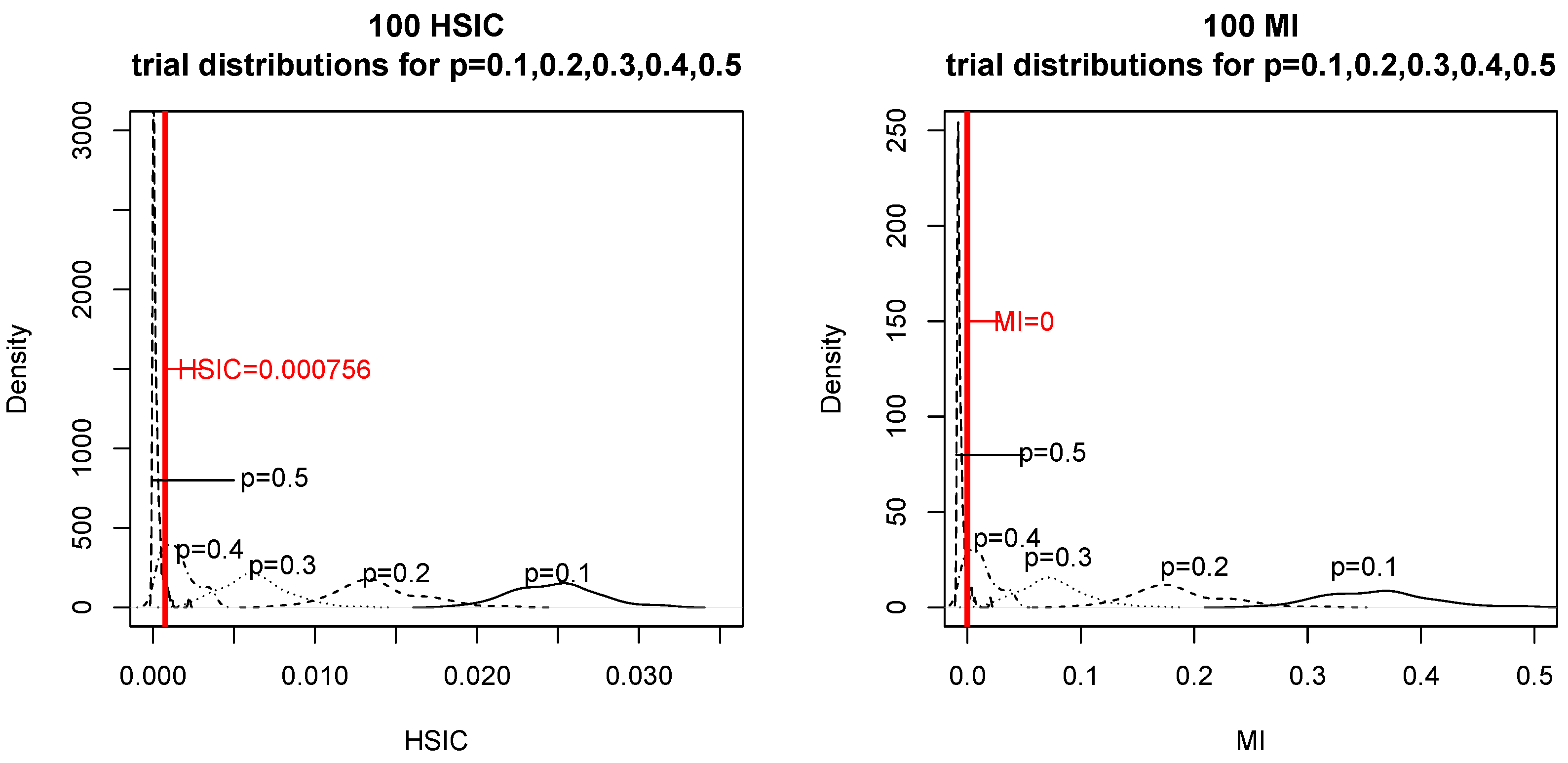
First, we generated mutually independent binary X and U, with the probabilities of $X=1$ and $U=1$ being 0.5 and $p=0.1,0.2,0.3,0.4,0.5$, respectively, to obtain $Y=X+U$ mod 2. When we simulated the null hypothesis, we generated $y^n$ in the same way as that used for generating $x^n$. We computed $J_n$ and $H_n$ 100 times for $n=100$ and $n=200$.

The obtained results are presented in Figure 5. For each p and $n=200$, we depict the distributions of $H_n$ and $J_n$ in the plots on the left and right, respectively. If the data occur to the left of the red vertical line, then the tests consider $x^n$ and $y^n$ to be independent. In particular, for $p=0.5$ ($X\perp \perp Y$) and $p=0.4$ (X Y), we counted how many times the two tests chose $X\perp \perp Y$ and X Y (see Table 1).

Figure 5. Experiments for binary sequences ($n=200$).

Table 1. Experiments for binary sequences: the figures show how many times (out of 100) the HSIC and the proposed method regarded the two sequences as being independent ($\perp \perp$) and dependent ( ) for $p=0.5,0.4,0.3$.

n = 200	p = 0.5		p = 0.4		n =100	p = 0.5		p = 0.4
(100 Trials)	$\perp \perp$		$\perp \perp$		(100 Trials)	$\perp \perp$		$\perp \perp$
HSIC	95	5	24	76	HSIC	95	5	49	51
Proposed	94	6	19	81	Proposed	88	12	33	67

We could not find any significant difference in the correctness of testing for the two tests.

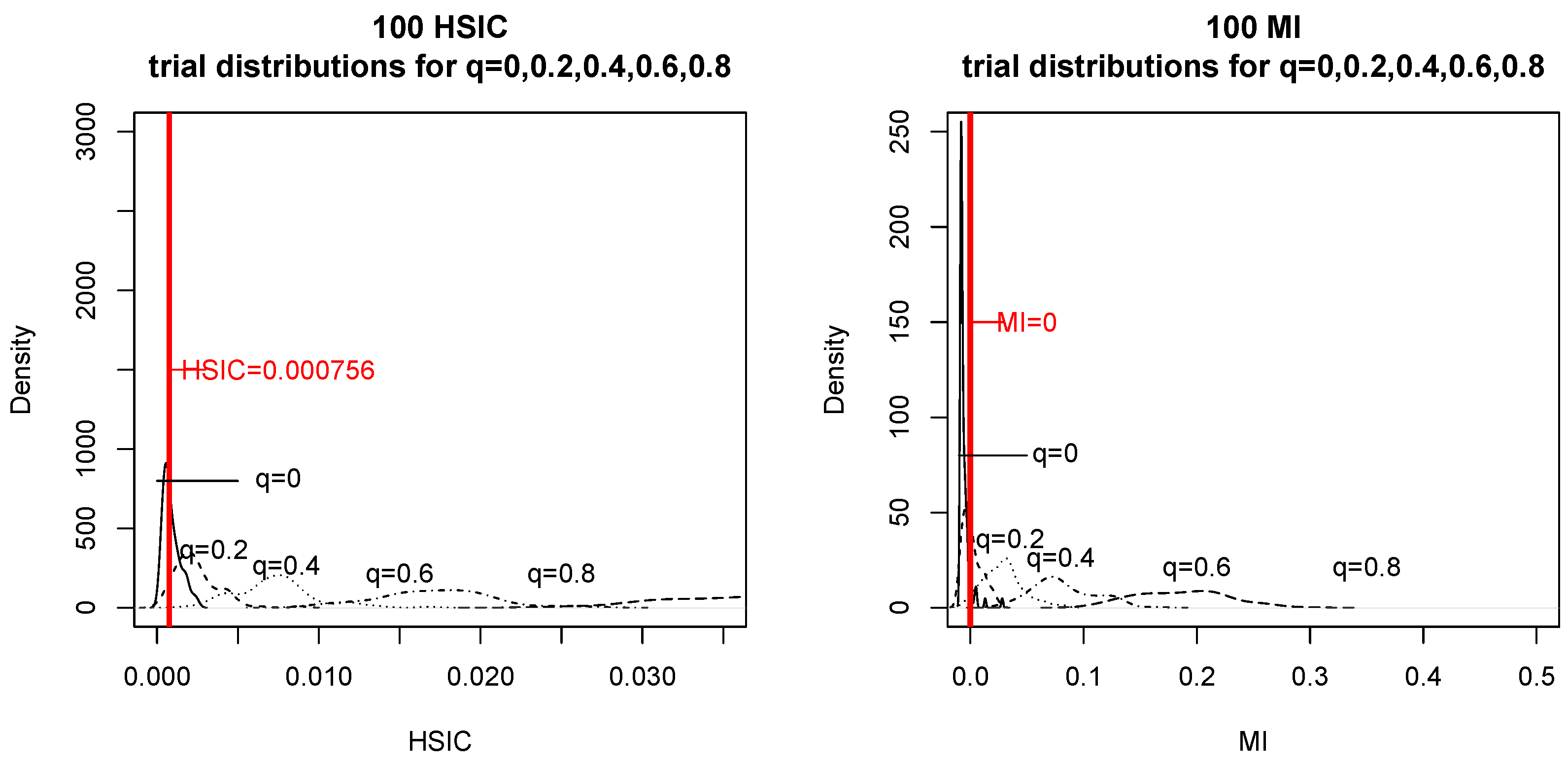
Next, we generated mutually independent Gaussian X and U with mean zero and variance one, and $Y=qX+\sqrt{1-q^2}U$ for $q=0,0.2,0.4,0.6,0.8$. When we simulated the null hypothesis, we generated $y^n$ in the same way as that used for generating $x^n$. We computed $J_n$ and $H_n$ 100 times for $n=100$ and $n=200$.

The obtained results are presented in Figure 6. For each q and $n=200$, we depict the distributions of $H_n$ and $J_n$ on the left and right, respectively. If the data occur to the left of the red vertical line, then the tests consider $x^n$ and $y^n$ to be independent. In particular, for $q=0.5$ ($X\perp \perp Y$) and $q=0.4$ (X Y), we counted how many times the two tests chose $X\perp \perp Y$ and X Y (see Table 2).

Figure 6. Experiments for Gaussian sequences ($n=200$).

Table 2. Experiments for Gaussian sequences: the figures show how many times (out of 100) the HSIC and the proposed method regarded the two sequences as being independent ($\perp \perp$) and dependent ( ) for $q=0,0.1,0.2$.

n = 200	q = 0		q = 0.2		q = 0.4		n = 100	q = 0		q = 0.2		q = 0.4
(100 Trials)	$\perp \perp$		$\perp \perp$		$\perp \perp$		(100 Trials)	$\perp \perp$		$\perp \perp$		$\perp \perp$
HSIC	97	3	51	49	0	100	HSIC	93	7	74	26	11	89
Proposed	95	5	58	42	4	92	Proposed	94	6	56	44	23	77

We could not find any significant difference in the correctness of testing between the two tests.

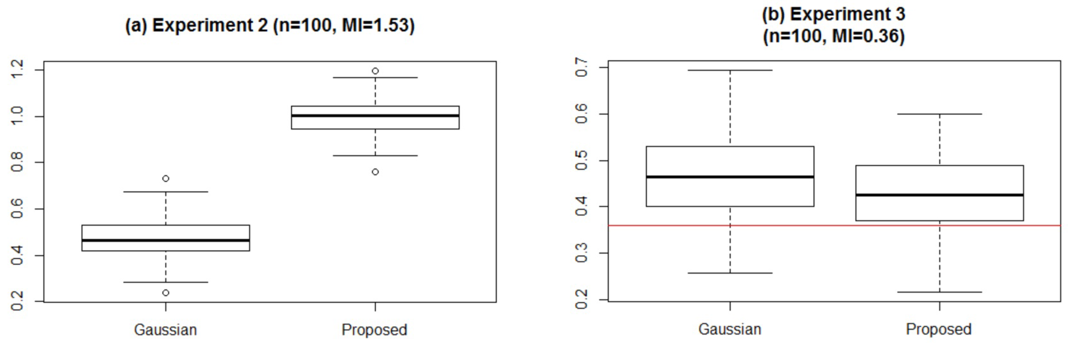
4.2. When is the Proposed Method Superior?

We found two cases in which the proposed method outperforms the HSIC:

• X and U are mutually independent and follow the Gaussian distribution with mean 0 and variance 0.25, and $Y=X-round(X)+round(U)$, where $round(x)$ is the rounded integer of x ($round(1.1)$ = 1$,round(1.6)=2,round(-1.1)=-1,round(-1.6)=-2$) (ROUNDING).
• X takes a value in $\{0,1,\cdots ,9\}$ uniformly and Y takes a value in either $\{0,2,4,6,8\}$ or $\{1,3,5,7,9\}$ uniformly depending on the value of X such that $X+Y$ is an even number (INTEGER).

We refer to the two problems as ROUNDING and INTEGER, respectively. Apparently, the answers to both of these are that $X,Y$ are not independent, although the correlation coefficient $\rho (X,Y)$ is zero.

Table 3 shows the number of times the tests chose $X\perp \perp Y$ and X Y for the experiments. We observed that the HSIC failed to detect dependencies for both of the problems, whereas the proposed method successfully found X and Y to not be independent.

Table 3. Hilbert-Schmidt independence criterion (HSIC) fails to detect dependencies.

n = 200	ROUNDING		n = 200	INTEGER
(100 Trials)	$\perp \perp$		(100 Trials)	$\perp \perp$
HSIC	100	0	HSIC	96	4
Proposed	1	99	Proposed	0	100

The obvious reason appears to be that the HSIC simply considers the magnitudes of $X,Y$. For the ROUNDING problem, $X,Y$ are independent for the integer parts, but the fractional parts are related. However, when using HSIC, because the integer part contributes to the score considerably more than the fractional part, the HSIC cannot detect the relation between the whole parts.

The same reasoning can be applied to the INTEGER problem. In fact, the values of $\lfloor X/2\rfloor$ and $\lfloor Y/2\rfloor$ are independent, where $\lfloor x\rfloor$ denotes the largest integer not exceeding x. However, the relation $X\equiv Y$ mod 2 always holds, and this cannot be detected by the HSIC.

Note that we do not claim that the proposed method is always superior to the HSIC. Admittedly, for many problems, the HSIC performs better. For example, for typical problems such as

3

X and U follow the standard Gaussian and binary (probability 0.5) distributions, and $Y=XU$ (ZERO-COV),

we find that the HSIC offers more advantages (see Table 4).

Table 4. HSIC outperforms the proposed method.

n = 200	ZERO-COV
(100 Trials)	$\perp \perp$
HSIC	0	100
Proposed	12	88

We rather claim that no single independence test outperforms all the others.

4.3. Execution Time

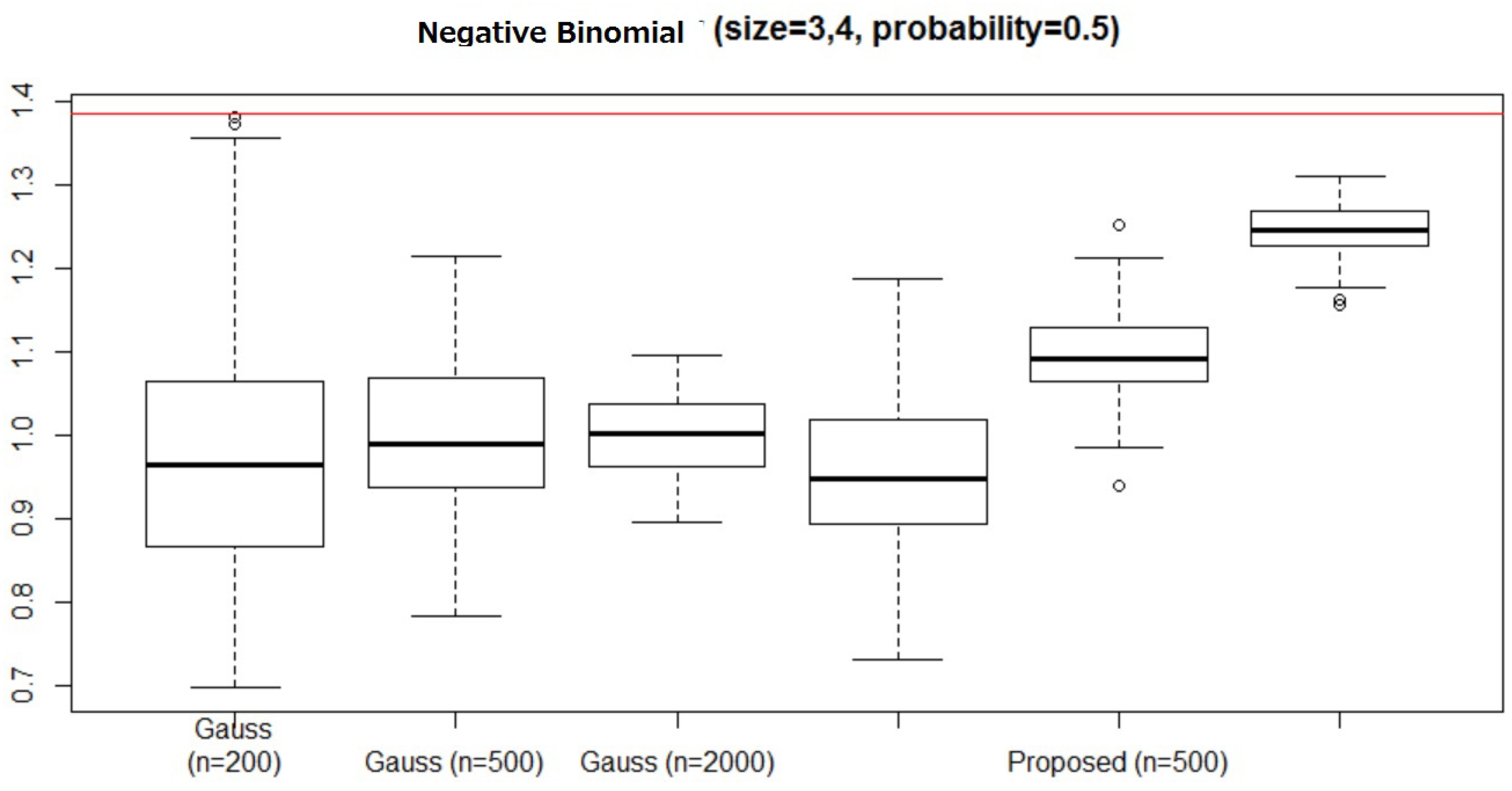
We compare the execution times for the Gaussian sequences. Table 5 lists the average execution times for $n=100,500,1000$, and 2000 and $q=0.2$ (the results were almost identical for the other values of q).

Table 5. Execution time (seconds).

n	100	500	1000	2000
HSIC	0.50	9.51	40.28	185.53
Proposed	0.30	0.33	0.62	1.05

We find that the proposed method is considerably faster than the HSIC, particularly for large n. This result occurs because the proposed method requires $O(n\log n)$ time for the computation, whereas the HSIC requires $O(n^3)$ time. Although the HSIC estimator might detect some independence for large n because of its (weak) consistency, it appears that the HSIC is not efficient for large n. Because the HSIC requires the null hypothesis to be simulated, a considerable amount of additional computation would be required.

5. Concluding Remarks

We proposed an estimator of mutual information and demonstrated the effectiveness of the algorithm in solving the independence testing problem.

Although estimating mutual information of continuous variables was considered to be difficult, the proposed estimator was shown to detect independence for a large sample size if and only if the two variables are independent. The estimator constructs many histograms of size $2^u\times 2^u$, estimates their mutual information $J_n^{(u)}$, and chooses the one with the maximum $J_n^{(u)}$ value over $u=1,2,\cdots$. We find that the optimal u has an upper bound of $\lfloor 0.5\log n\rfloor$. The proposed algorithm requires $O(n\log n)$ time to perform the computation.

Then, we compared the performance of our proposed estimator with that of the HSIC estimator, de facto for the independence testing principle. The two methods differ in that the proposed method is based on the MDL principle given data $x^n,y^n$, although the HSIC detects abnormalities assuming the null hypothesis given the data. We could not obtain a definite answer to enable us to determine which method is superior for general settings; rather, we obtained evidence that no single statistical test outperforms all the others for all problems. In fact, although HSIC will clearly be superior when certain specific dependency structures form the alternative hypothesis, the proposed estimator is more universal.

One meaningful insight obtained is that the HSIC only considers the magnitude of the data and neglects to find relations that cannot be detected by simply considering the changes in magnitude.

The most notable merit of the proposed algorithm compared to the HSIC is its efficiency. The HSIC requires $O(n^3)$ computational time for one test. However, prior to the test, it is necessary to simulate the null hypothesis and set the threshold such that the algorithm determines that the data are independent if and only if the HSIC values do not exceed the threshold. In this sense, executing the HSIC would be time-consuming, and it would be safe to say that the proposed algorithm is useful for designing intelligent machines, whereas the HSIC is appropriate for scientific discovery.

In future work, we will consider exactly when the proposed method exhibits a particularly good performance.

Moreover, we should address the question of how generalizations to three dimensions might work. In this paper, it is not clear whether one would want to estimate some form of total independence such as ${\displaystyle E\log \frac{p(X,Y,Z)}{p(X)p(Y)p(Z)}}$ or conditional mutual information such as ${\displaystyle E\log \frac{p(X,Y,Z)p(X)}{p(X,Z)p(X,Y)}}$. In fact, for Bayesian network structure learning (BNSL), we need to compute Bayesian scores of conditional mutual information from the data to apply a standard scheme of BNSL based on dynamic programming [16]. Currently, a constraint-based approach for estimating conditional mutual information values using positive definite kernels is available [17], but no theoretical guarantee, such as consistency, is obtained by the method.

References

- Shannon, C.E. A Mathematical Theory of Communication. Bell Syst. Tech. J. 1948, 27, 379–423. [Google Scholar] [CrossRef]
- Rissanen, J. Modeling by shortest data description. Automatica 1978, 14, 465–471. [Google Scholar] [CrossRef]
- Suzuki, J. A Construction of Bayesian Networks from Databases on an MDL Principle. In Proceedings of the Conference on Uncertainty in Artificial Intelligence, Washington, DC, USA, 9–11 July 1993; pp. 266–273.
- Härdle, W.; Müller, M.; Sperlich, S.; Werwatz, A. Nonparametric and Semiparametric Models; Springer-Verlag: Berlin/Heidelberg, Germany, 2004. [Google Scholar]
- Evans, D. A computationally efficient estimator for mutual information. Proc. R. Soc. A 2013, 464, 1203–1215. [Google Scholar] [CrossRef]
- Kraskov, A.; Stögbauer, H.; Grassberger, P. Estimating mutual information. Phys. Rev. E 2004, 69, 066138. [Google Scholar] [CrossRef] [PubMed]
- Silva, J.; Narayanan, S.S. Nonproduct Data-Dependent Partitions for Mutual Information Estimation: Strong Consistency and Applications. IEEE Trans. Signal Process. 2010, 58, 3497–3511. [Google Scholar] [CrossRef]
- Gretton, A.; Bousquet, O.; Smola, A.J.; Scholkopf, B. Measuring Statistical Dependence with Hilbert-Schmidt Norms. In Proceedings of the 16th Conference on Algorithmic Learning Theory, Singapore, Singapore, 8–11 October 2005.
- Suzuki, J. The Bayesian Chow-Liu Algorithm. In Proceedings of the Sixth European Workshop on Probabilistic Graphical Models, Granada, Spain, 19–21 September 2012.
- Krichevsky, R.E.; Trofimov, V.K. The Performance of Universal Encoding. IEEE Trans. Inf. Theory 1981, 27, 199–207. [Google Scholar] [CrossRef]
- Nemenman, I.; Shafee, F.; Bialek, F.W. Entropy and inference, revisited. In Advances in Neural Information Processing Systems 14; MIT Press: Cambridge, MA, USA, 2002; pp. 471–478. [Google Scholar]
- Archer, E.; Park, M.I.; Pillow, J. Bayesian and Quasi-Bayesian Estimators for Mutual Information from Discrete Data. Entropy 2013, 15, 1738–1755. [Google Scholar] [CrossRef]
- Hutter, M. Distribution of mutual information. In Advances in Neural Information Processing Systems 14; MIT Press: Cambridge, MA, USA, 2002; pp. 399–406. [Google Scholar]
- Gessaman, M.P. A Consistent Nonparametric Multivariate Density Estimator Based on Statistically Equivalent Blocks. Ann. Math. Stat. 1970, 41, 1344–1346. [Google Scholar] [CrossRef]
- Wolpert, D.; Macready, W. No Free Lunch Theorems for Optimization. IEEE Trans. Evol. Comput. 1997, 1, 67–82. [Google Scholar] [CrossRef]
- Silander, T.; Myllymaki, P. A simple approach for finding the globally optimal Bayesian network structure. In Proceedings of the 22nd Conference on Uncertainty in Artificial Intelligence, Cambridge, MA, USA, 13–16 July 2006.
- Zhang, K.; Peters, J.; Janzing, D.; Scholkopf, B. Kernel-based Conditional Independence Test and Application in Causal Discovery. In Proceedings of the Conference on Uncertainty in Artificial Intelligence, Barcelona, Spain, 14–17 July 2011; pp. 804–813.
- Suzuki, J. On Strong Consistency of Model Selection in Classification. IEEE Trans. Inf. Theory 2006, 52, 4767–4774. [Google Scholar] [CrossRef]
- Suzuki, J. Consistency of Learning Bayesian Network Structures with Continuous Variables: An Information Theoretic Approach. Entropy 2015, 17, 5752–5770. [Google Scholar] [CrossRef]
© 2016 by the author; licensee MDPI, Basel, Switzerland. This article is an open access article distributed under the terms and conditions of the Creative Commons by Attribution (CC-BY) license (http://creativecommons.org/licenses/by/4.0/).