1. Intoduction
Parameter inference is an important task in the interpretation of magnetic resonance spectra and may be accomplished by a variety of means. One approach of particular note is the early and important work of Bretthorst who established methods for the analysis of high resolution Nuclear Magnetic Resonance (NMR) lineshapes that are complementary to the Markov Chain Monte Carlo methods developed in this work [
1,
2,
3]. Markov Chain Monte Carlo simulations are frequently used in statistics for sampling probability distributions to compute quantities that would otherwise be difficult to evaluate by conventional means. In this paper we will discuss a Markov Chain Monte Carlo algorithm optimized for parameter inference of the absorption lineshape of a Pake Doublet, which arises from the magnetic dipole-dipole interaction between coupled spins. This Lineshape is important in both NMR and Electron Paramagnetic Resonance (EPR). In modern applications, the details of the lineshape can provide distance information for various spin systems [
4]. For the purposes of this paper, we will explore the process of parameter inference for a case of historical interest and reanalyze Pake’s original distance determination of a hydrated gypsum crystal [
5].
The probability of absorption is [
5,
6]:
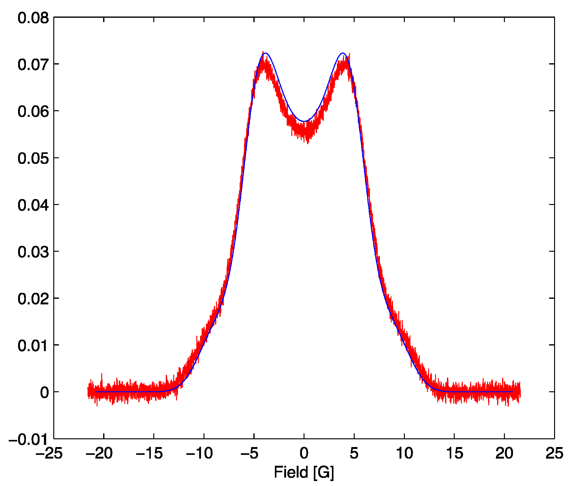
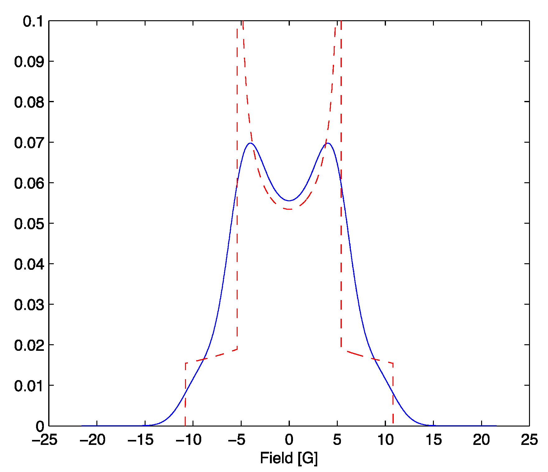
This distribution (1) is convolved with a Gaussian to represent inhomogeneities in the magnetic field as well as contributions from neighboring atoms. The Gaussian has the form:
and the lineshape has the form:
shown in
Figure 1.
Figure 1.
Absorption probability for α = 5.4 in red. The result of (3) in blue with β = 1.54.
Figure 1.
Absorption probability for α = 5.4 in red. The result of (3) in blue with β = 1.54.
Note that the absorption lineshape (3) is normalized and is non-negative, and so may be treated as a probability mass function [
7].
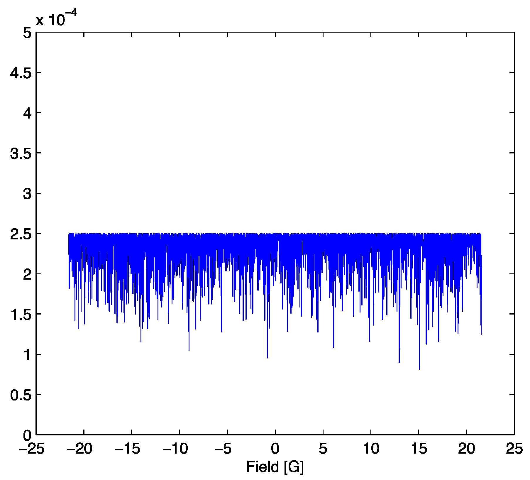
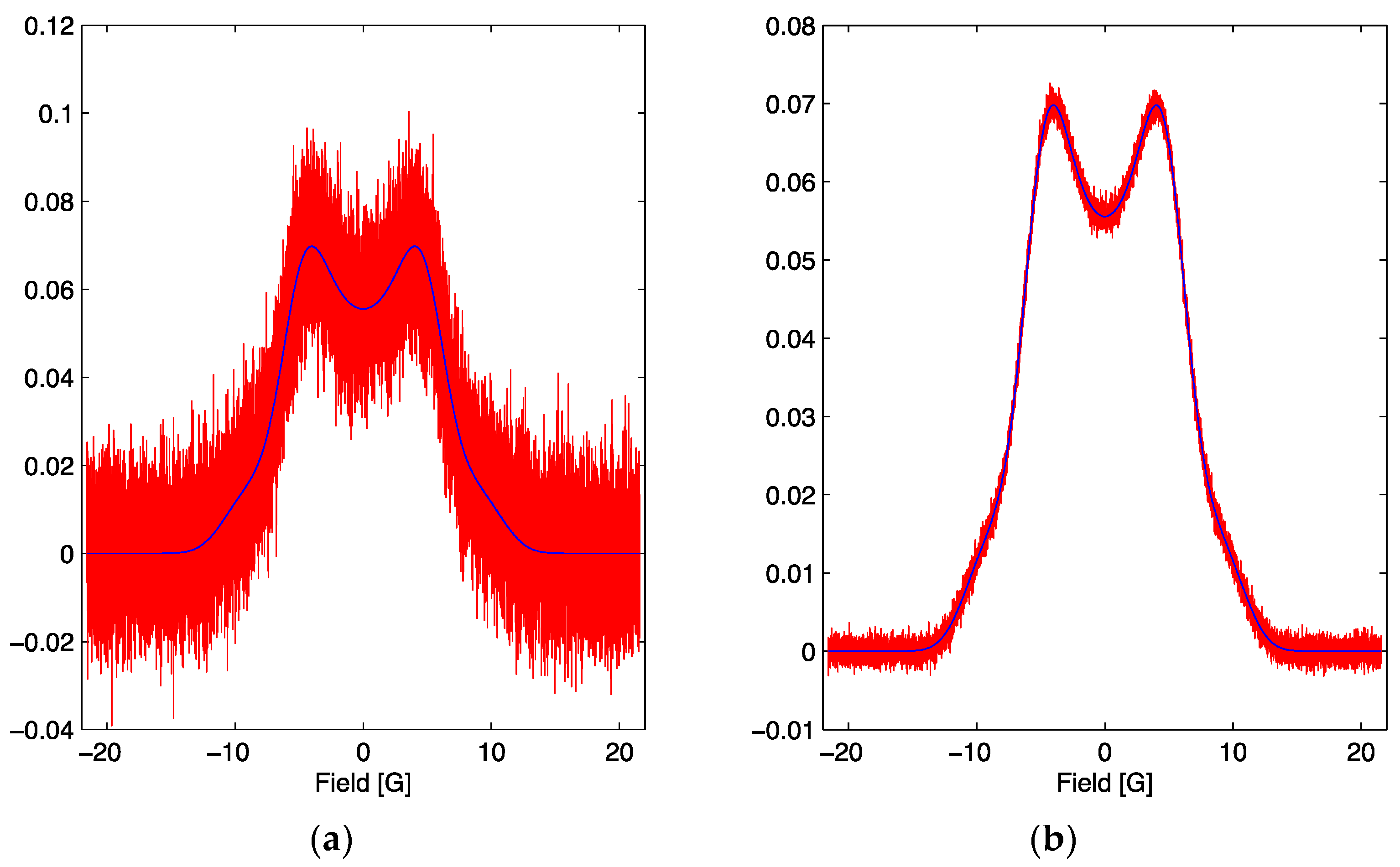
In this work we will study two cases, one with a SNR = 7,
Figure 2a, and the second with a SNR = 70,
Figure 2b, with emphasis on the latter since it is more sensitive to the explicit values of the parameters. SNR is the signal to noise ratio and is defined as the ratio of the maximum amplitude of the signal to the root mean square noise width of the signal.
Figure 2.
(a) The simulated signal for the optimum parameter set with the addition of noise (red) and the noiseless lineshape (blue). The red signal corresponds to a signal to noise ratio of 7. (b) The simulated signal for the optimum parameter set with the addition of noise (red) and the noiseless lineshape (blue). The red signal corresponds to a signal to noise ratio of 70.
We will use the maximum likelihood distribution [
8]:
which can be derived from manipulation of Bayes’ Theorem. In (4),
F is the model (3), σ is the width of the noise (
Nk/n, where
Nk is the normal noise generated in MATLAB (version R2013a), which has a width = 1 which is then scaled by n to obtain the desired SNR), {
X} represents a set of parameters (in this case α and β), our signal
, and the
k subscript indicates a specific observation frequency in the bandwidth of the spectrum. Here, {
Xo} is the optimum parameter set, {α
o, β
o}.
The maximum likelihood distribution (4) is analogous to the canonical ensemble (5) [
9]:
We can obtain equality if we set
and
or
, the analog to temperature used in Boltzmann statistics [
9,
10]. Note that we measure our pseudotemperature
T in units of
Ek. We can normalize Equation (4) by constructing a probability mass function whose evidence (or partition function) may be defined by using Equations (4) and (6):
The probability mass function then takes the form:
where {
Xi} is the
i-th set of parameters being evaluated, {α
i, β
i}.
By analogy to the canonical distribution, we observe that there are many computable quantities with connections to classical thermodynamics such as the heat capacity, which in this case gives a measure of the fluctuations of the mean-squared residual in the presence of noise; the expectation of the residual, which is controlled by the pseudo temperature
; and the Shannon and Boltzmann entropy [
10]. The residual squared:
is expected to be a minimum at the parameter optimum {
X0}.
At the optimum parameter set,
[
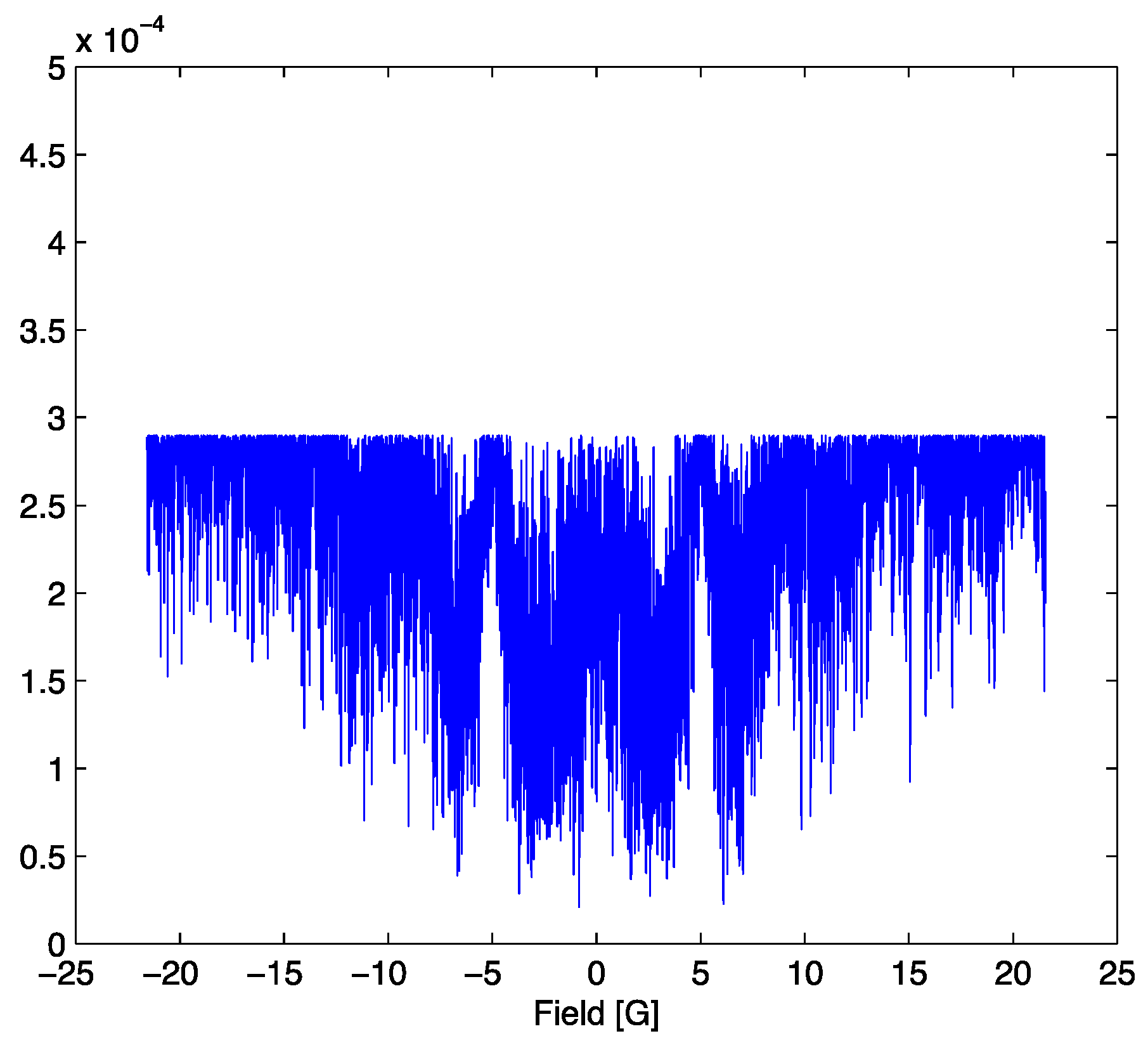
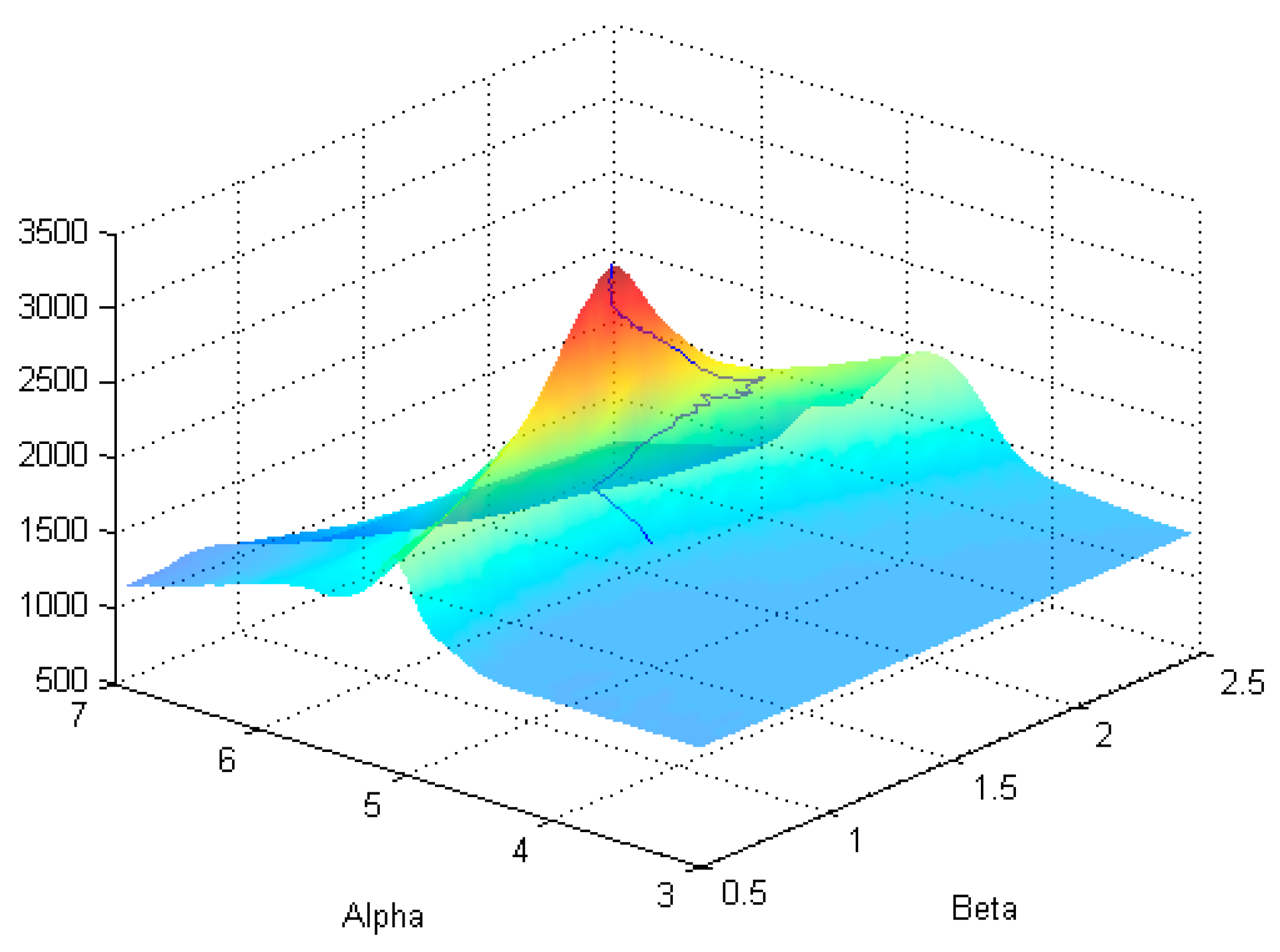
5] and a signal to noise ratio of 70 our probability mass function (8) is shown in
Figure 3. This is the optimum set used in all simulations discussed. An example simulated signal with parameter set
with a signal to noise ratio of 70 is shown in
Figure 4 and the resulting probability mass function (8) in
Figure 5.
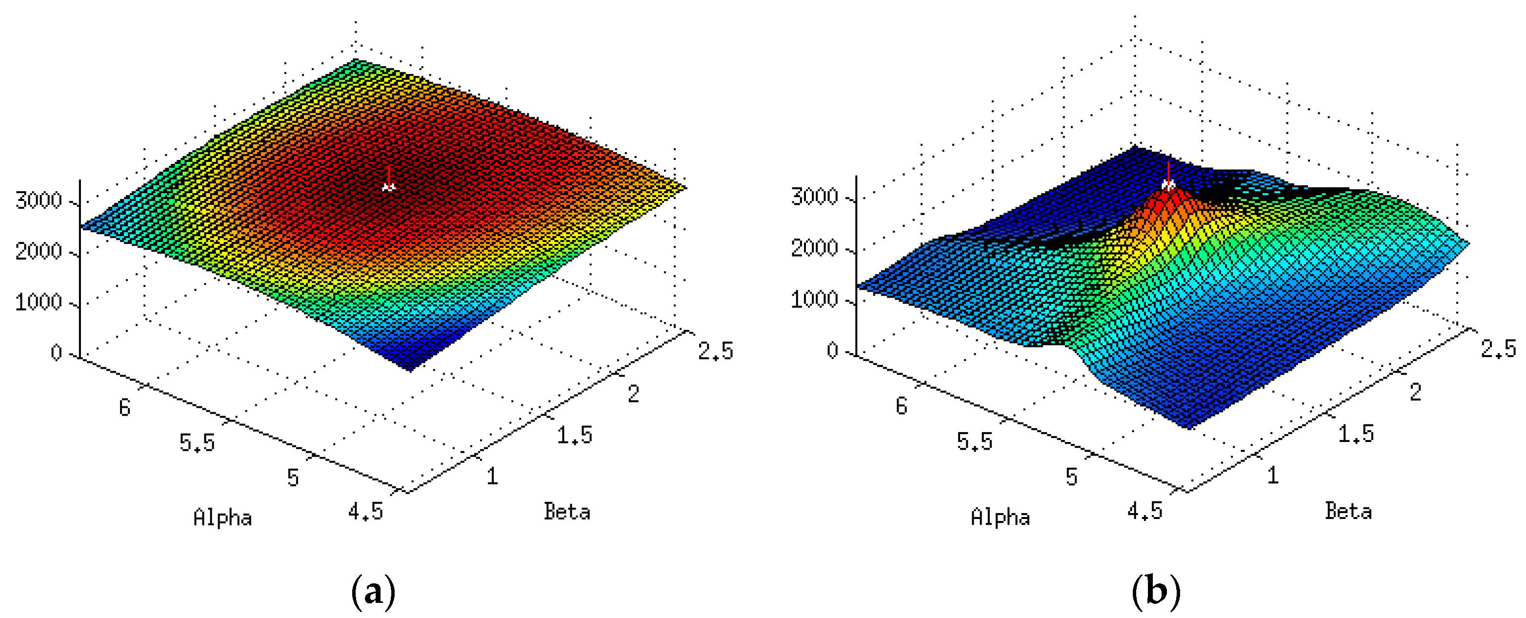
Figure 3.
Probability mass function (8) evaluated at the optimal parameter set and SNR = 70.
Figure 3.
Probability mass function (8) evaluated at the optimal parameter set and SNR = 70.
Figure 4.
The simulated signal for the optimum parameter set with SNR = 70 in red and the model lineshape evaluated at α = 5.2, β = 1.49 in blue.
Figure 4.
The simulated signal for the optimum parameter set with SNR = 70 in red and the model lineshape evaluated at α = 5.2, β = 1.49 in blue.
Figure 5.
Probability mass function (8) evaluated at α = 5.2 and β = 1.49 and SNR = 70.
Figure 5.
Probability mass function (8) evaluated at α = 5.2 and β = 1.49 and SNR = 70.
Note that the maximum amplitude of the probability mass function in
Figure 5 is slightly higher than that in
Figure 3. This is a result of a decrease in the value of the normalization constant, the partition function (7), which leads to a slight increase in the probability of points far from the center of the distribution where the model and signal still coincide. The decrease in the partition function arises because deviations from the optimum parameter set distort the probability mass function. This may be interpreted in a thermodynamic analogy as a non-equilibrium state where the residual is treated as a distortion energy. When the parameter set is non-optimum, the distortion energy increases, corresponding to a “perturbation” away from equilibrium. During a successful search process, the mean squared residual approaches a minimum and “equilibrium” is achieved at the optimum parameter set. In order to accurately estimate the uncertainties in the parameters, it is necessary to quantify precisely how the mean-squared distortion energy changes in the neighborhood of the parameter optimum. In some sense, we need a measure of how far “apart” different posteriors are. The tool of choice for this purpose is the Fisher information matrix which can be treated as a metric in the space of lineshape model parameters [
7]. The Fisher information matrix induces a geometry on parameter space. For the particular case studied here, we will show in
Section 3 that the resulting geometry has negative curvature, analogous to the surface of a saddle, and this has consequences for accurate computation of parameter uncertainties. The
Appendix contains a brief formulary for some needed results from differential geometry for the computation of quantities related to curvature. Some of these results are only valid for the two dimensional parameter space treated here. The references should be consulted for the extensions needed to accommodate parameter spaces of higher dimension.
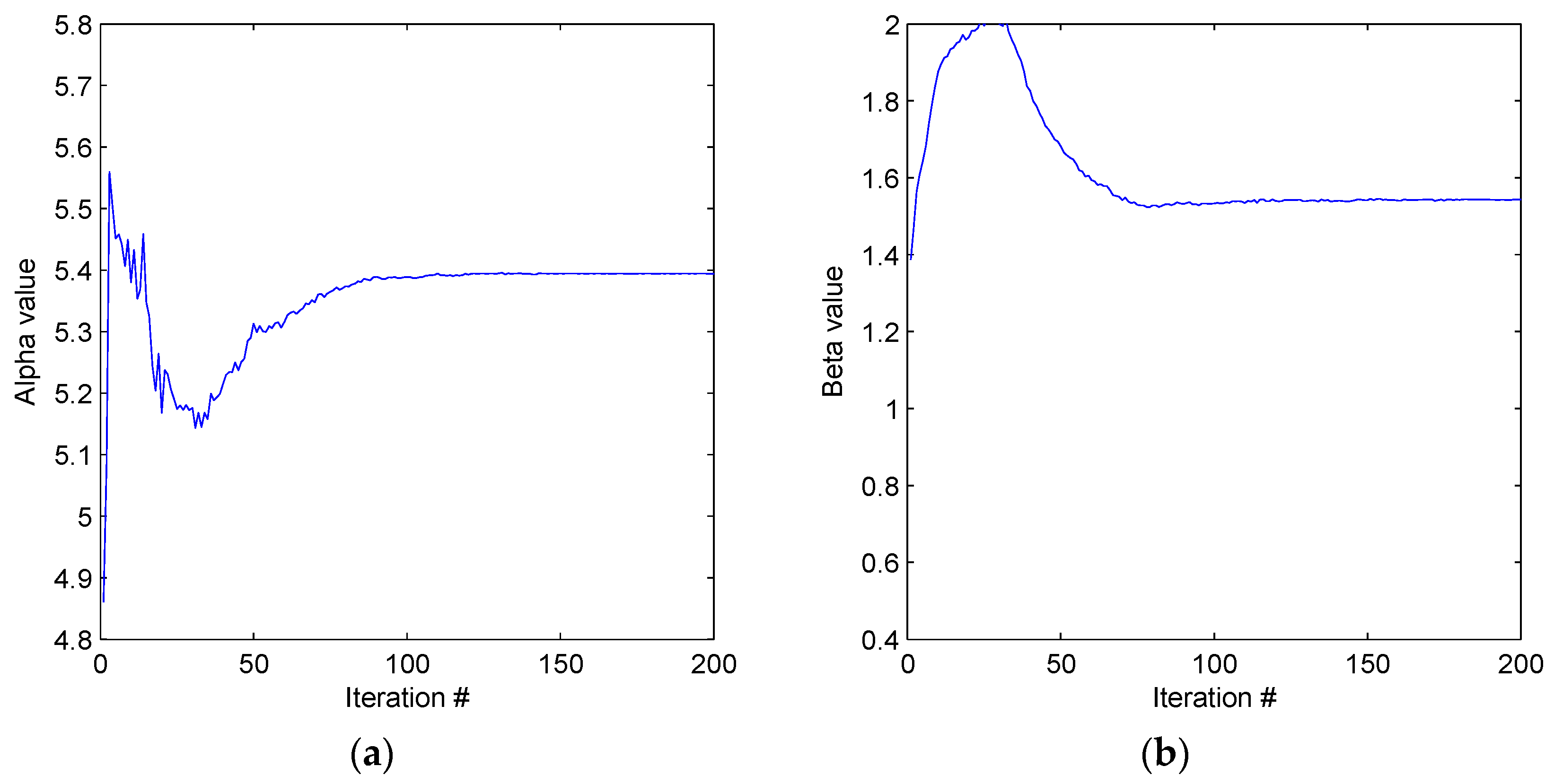
4. Discussion
Our motivation for studying this problem was to extend the methods of [
7] which were applied to a simple absorption line to a more complex problem. As noted in the introduction, the work of Bretthorst provides an alternative perspective and approach [
1,
2,
3]. In addition, we wanted to further explore the consequences of the curvature corrections implied by the probability mass function introduced in [
10], which explicitly accounts for noise in the spectrum. These considerations encouraged us to develop an algorithm for finding the optimum parameter set of an inhomogeneously broadened Pake doublet spectrum in the presence of noise. This algorithm proves to be accurate and reliable in cases with good signal to noise; its accuracy drops off in both the high and low SNR regions. For these cases, a nested sampling algorithm [
8] was used but is not discussed in this paper. The algorithm also requires a sampling procedure that can accurately accommodate the inverse square root singularity of Euqation (1). It does exemplify how the principles of a Metropolis Hastings Markov Chain Monte Carlo algorithm can be adapted to suit the requirements of parameter optimization for a magnetic resonance lineshape of importance for distance determinations [
4,
5]. It should be noted that the cases treated in this work do not account for the systematic errors that certainly complicate parameter inference in practical applications. As illustrative but by no means exhaustive examples, we have considered the effects of an unmodeled background signal, as well as an admixture of dispersion into the Pake doublet spectrum, as summarized elsewhere [
10]. Athough we have shown that systematic errors can be accommodated by our methods [
10], we felt that explicit consideration of such errors would detract from our principle aim in the work reported on here, which was to estimate and demonstrate the effets of parameter space curvature in idealized cases.
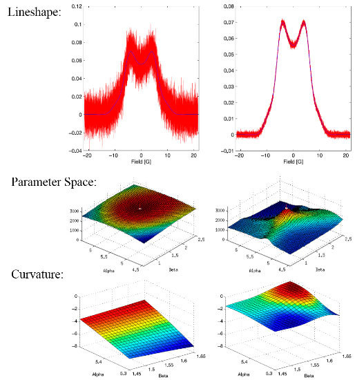
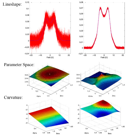
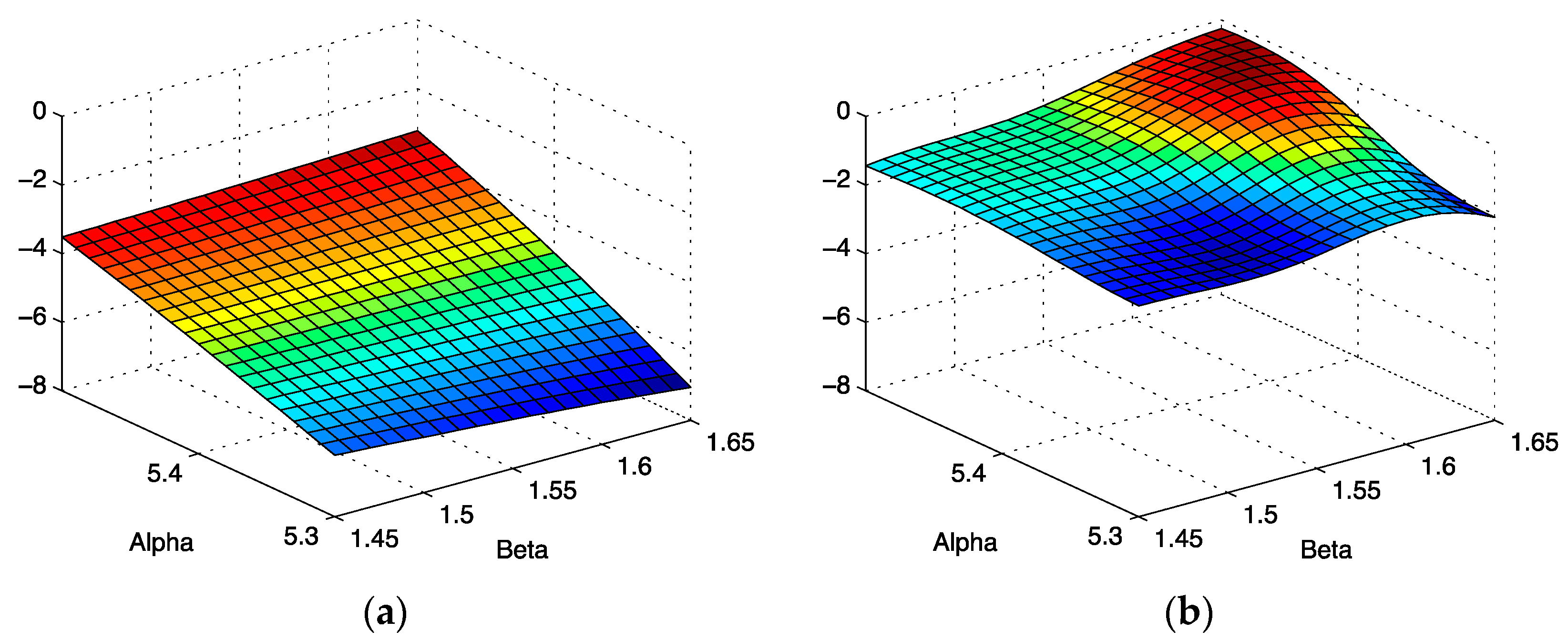
Our results provide some justification for standard error estimate practices for spectra with good signal to noise [
11], exemplified by the spectrum shown in
Figure 2. The scalar curvature for this case, shown in
Figure 12b, is smaller in magnitude over the entire parameter space explored than the scalar curvature for the low signal to noise ratio case shown in
Figure 12a. A scalar curvature of zero corresponds to a flat, or Euclidean geometry. In computing error estimates, the standard computation uses a Hessian constructed under the assumption that curvature effects may be neglected, or equivalently, that the Christoffel symbols are all zero in this space. We see that for high signal to noise, this is a well-justified assumption, but our results do indicate that it is an approximation. For the case of low signal to noise ratio, error estimates computed without curvature corrections are even more of an approximation than one might otherwise suppose. In applications, the parameter uncertainties are important criteria for assessing the reliability of the parameter inference for models of the environments in which the spin-bearing moments are found with consequences for what structural information may be trusted. In addition, the signal to noise is often sub-optimal for samples of biological interest. For these cases, the methods developed in this work permit significant refinements over conventional methods.
The methods reported on here may be applied to any lineshape model for which analytical derivatives are available. Numerical derivatives may be used when necessary, but the number of required derivatives for curvature calculations, as many as four, can result in significant loss of accuracy if the computations are performed without care. MATLAB scripts comprising an implementation of the algorithm described here are available for download from the Earle research website: earlelab.rit.albany.edu.

