Article

The Information Geometry of Sparse Goodness-of-Fit Testing

1
Department of Statistics and Actuarial Science, University of Waterloo, 200 University Avenue West, Waterloo, ON N2L 3G1, Canada
2
School of Mathematics and Statistics, The Open University, Walton Hall, Milton Keynes, Buckinghamshire MK7 6AA, UK
3
Department of Mathematics & ECARES, Université libre de Bruxelles, Avenue F.D. Roosevelt 42, 1050 Brussels, Belgium
*
Author to whom correspondence should be addressed.
Entropy 2016, 18(12), 421; https://doi.org/10.3390/e18120421
Submission received: 31 August 2016 / Revised: 16 November 2016 / Accepted: 19 November 2016 / Published: 24 November 2016
(This article belongs to the Special Issue Differential Geometrical Theory of Statistics)

Abstract

:
This paper takes an information-geometric approach to the challenging issue of goodness-of-fit testing in the high dimensional, low sample size context where—potentially—boundary effects dominate. The main contributions of this paper are threefold: first, we present and prove two new theorems on the behaviour of commonly used test statistics in this context; second, we investigate—in the novel environment of the extended multinomial model—the links between information geometry-based divergences and standard goodness-of-fit statistics, allowing us to formalise relationships which have been missing in the literature; finally, we use simulation studies to validate and illustrate our theoretical results and to explore currently open research questions about the way that discretisation effects can dominate sampling distributions near the boundary. Novelly accommodating these discretisation effects contrasts sharply with the essentially continuous approach of skewness and other corrections flowing from standard higher-order asymptotic analysis.

1. Introduction

We start by emphasising the threefold achievements of this paper, spelled out in detail in terms of the paper’s section structure below. First, we present and prove two new theorems on the behaviour of some standard goodness-of-fit statistics in the high dimensional, low sample size context, focusing on behaviour “near the boundary” of the extended multinomial family. We also comment on the methods of proof which allow explicit calculations of higher order moments in this context. Second, working again explicitly in the extended multinomial context, we fill a hole in the literature by linking information-geometric-based divergences and standard goodness-of-fit statistics. Finally, we use simulation studies to explore discretisation effects that can dominate sampling distributions “near the boundary”. Indeed, we illustrate and explore how—in the high dimensional, low sample size context—all distributions are affected by boundary effects. We also use these simulation results to explore currently open research questions. As can be seen, the overarching theme is the importance of working in the geometry of the extended exponential family [1], rather than the traditional manifold-based structure of information geometry.
In more detail, the paper extends and builds on the results of [2], and we use notation and definitions consistently across these two papers. Both papers investigate the issue of goodness-of-fit testing in the high dimensional sparse extended multinomial context, using the tools of Computational Information Geometry (CIG) [1].
Section 2 gives formal proofs of two results, Theorems 1 and 2, which were announced in [2]. These results explore the sampling performance of standard goodness-of-fit statistics—Wald, Pearson’s χ 2 , score and deviance—in the sparse setting. In particular, they look at the case where the data generation process is “close to the boundary” of the parameter space where one or more cell probabilities vanish. This complements results in much of the literature, where the centre of the parameter space—i.e., the uniform distribution—is often the focus of attention.
Section 3 starts with a review of the links between Information Geometry (IG) [3] and goodness-of-fit testing. In particular, it looks at the power family of Cressie and Read [4,5] in terms of the geometric theory of divergences. In the case of regular exponential families, these links have been well-explored in the literature [6], as has the corresponding sampling behaviour [7]. What is novel here is the exploration of the geometry with respect to the closure of the exponential family; i.e., the extended multinomial model—a key tool in CIG. We illustrate how the boundary can dominate the statistical properties in ways that are surprising compared to standard—and even high-order—analyses, which are asymptotic in sample size.
Through simulation experiments, Section 4 explores the consequences of working in the sparse multinomial setting, with the design of the numerical experiments being inspired by the information geometry.

2. Sampling Distributions in the Sparse Case

One of the first major impacts that information geometry had on statistical practice was through the geometric analysis of higher order asymptotic theory (e.g., [8,9]). Geometric interpretations and invariant expressions of terms in the higher order corrections to approximations of sampling distributions are a good example, [8] (Chapter 4). Geometric terms are used to correct for skewness and other higher order moment (cumulant) issues in the sampling distributions. However, these correction terms grow very large near the boundary [1,10]. Since this region plays a key role in modelling in the sparse setting—the maximum likelihood estimator (MLE) often being on the boundary—extensions to the classical theory are needed. This paper, together with [2], start such a development. This work is related to similar ideas in categorical, (hierarchical) log–linear, and graphical models [1,11,12,13]. As stated in [13], “their statistical properties under sparse settings are still very poorly understood. As a result, analysis of such data remains exceptionally difficult”.
In this section we show why the Wald—equivalently, the Pearson χ 2 and score statistics—are unworkable when near the boundary of the extended multinomial model, but that the deviance has a simple, accurate, and tractable sampling distribution—even for moderate sample sizes. We also show how the higher moments of the deviance are easily computable, in principle allowing for higher order adjustments. However, we also make some observations about the appropriateness of these classical adjustments in Section 4.
First, we define some notation, consistent with that of [2]. With i ranging over { 0 , 1 , , k } , let n = ( n i ) Multinomial ( N , ( π i ) ) , where here each π i > 0 . In this context, the Wald, Pearson’s χ 2 , and score statistics all coincide, their common value, W, being
W : = i = 0 k ( π i n i / N ) 2 π i 1 N 2 i = 0 k n i 2 π i 1 .
Defining π ( α ) : = i π i α , we note the inequality, for each m 1 ,
π ( m ) ( k + 1 ) m + 1 0 ,
in which equality holds if and only if π i 1 / ( k + 1 ) —i.e., iff ( π i ) is uniform. We then have the following theorem, which establishes that the statistic W is unworkable as π min : = min ( π i ) 0 for fixed k and N.
Theorem 1.
For k > 1 and N 6 , the first three moments of W are:
E ( W ) = k N , V a r ( W ) = π ( 1 ) ( k + 1 ) 2 + 2 k ( N 1 ) N 3
and E [ W E ( W ) 3 ] given by
π ( 2 ) ( k + 1 ) 3 ( 3 k + 25 22 N ) π ( 1 ) ( k + 1 ) 2 + g ( k , N ) N 5 ,
where g ( k , N ) = 4 ( N 1 ) k ( k + 2 N 5 ) > 0 .
In particular, for fixed k and N, as π min 0
V a r ( W ) and γ ( W ) + ,
where γ ( W ) : = E [ W E ( W ) 3 ] / { V a r ( W ) } 3 / 2 .
A detailed proof is found in Appendix A, and we give here an outline of its important features. The machinery developed is capable of delivering much more than a proof of Theorem 1. As indicated there, it provides a generic way to explicitly compute arbitrary moments or mixed moments of multinomial counts, and could in principle be implemented by computer algebra. Overall, there are four stages. First, a key recurrence relation is established; secondly, it is exploited to deliver moments of a single cell count. Third, mixed moments of any order are derived from those of lower order, exploiting a certain functional dependence. Finally, results are combined to find the first three moments of W, higher moments being similarly obtainable.
The practical implication of Theorem 1 is that standard first (and higher-order) asymptotic approximations to the sampling distribution of the Wald, χ 2 , and score statistics break down when the data generation process is “close to” the boundary, where at least one cell probability is zero. This result is qualitatively similar to results in [10], which shows how asymptotic approximations to the distribution of the maximum likelihood estimate fail; for example, in the case of logistic regression, when the boundary is close in terms of distances as defined by the Fisher information.
Unlike statistics considered in Theorem 1, the deviance has a workable distribution in the same limit: that is, for fixed N and k as we approach the boundary of the probability simplex. In sharp contrast to that theorem, we see the very stable and workable behaviour of the k-asymptotic approximation to the distribution of the deviance, in which the number of cells increases without limit.
Define the deviance D via
D / 2 = { 0 i k : n i > 0 } n i log ( n i / N ) i = 0 k n i log ( π i ) = { 0 i k : n i > 0 } n i log ( n i / μ i ) ,
where μ i : = E ( n i ) = N π i . We will exploit the characterisation that the multinomial random vector ( n i ) has the same distribution as a vector of independent Poisson random variables conditioned on their sum. Specifically, let the elements of ( n i * ) be independently distributed as Poisson P o ( μ i ) . Then, N * : = i = 0 k n i * P o ( N ) , while ( n i ) : = ( n i * | N * = N ) Multinomial ( N , ( π i ) ) . Define the vector
S * : = N * D * / 2 = i = 0 k n i * n i * log ( n i * / μ i ) ,
where D * is defined implicitly and 0 log 0 : = 0 . The terms ν, τ, and ρ are defined by the first two moments of S * via the vectors
N ν : = E ( S * ) = N i = 0 k E ( n i * log n i * / μ i ) ,
N ρ τ N · τ 2 : = C o v ( S * ) = N i = 0 k C i · i = 0 k V i ,
where C i : = C o v ( n i * , n i * log ( n i * / μ i ) ) and V i : = V a r ( n i * log ( n i * / μ i ) ) .
Theorem 2.
Each of the terms ν, τ, and ρ remains bounded as π min 0 .
We start with some preliminary remarks. We use the following notation: N : = { 1 , 2 , } denotes the natural numbers, while N 0 : = { 0 } N . Throughout, X P o ( μ ) denotes a Poisson random variable having positive mean μ—that is, X is discrete with support N 0 and probability mass function p : N 0 ( 0 , 1 ) given by:
p ( x ) : = e μ μ x / x ! ( μ > 0 ) .
Putting:
m N 0 , F [ m ] ( μ ) : = Pr ( X m ) = x = 0 m p ( x ) ( 0 , 1 ) ,
for given μ, { 1 F [ m ] ( μ ) } is strictly decreasing with m, vanishing as m . For all ( x , m ) N 0 2 , we define x ( m ) by:
x ( 0 ) : = 1 ; x ( m ) : = x ( x 1 ) ( x ( m 1 ) ) ( m N )
so that, if x m , x ( m ) = x ! / ( x m ) ! .
The set A 0 comprises all functions a 0 : ( 0 , ) R such that, as ξ 0 + :
( i )   a 0 ( ξ )   tends to an infinite limit   a 0 ( 0 + ) { , + } ,   while :   ( ii )   ξ a 0 ( ξ ) 0 .
Of particular interest here, by l’Hôspital’s rule,
m N , ( log ) m A 0 ,
where ( log ) m : ξ ( log ξ ) m ( ξ > 0 ) . For each a 0 A 0 , a 0 ¯ denotes its continuous extension from ( 0 , ) to [ 0 , ) —that is: a 0 ¯ ( 0 ) : = a 0 ( 0 + ) ; a 0 ¯ ( ξ ) : = a 0 ( ξ ) ( ξ > 0 ) —while, appealing to continuity, we also define 0 a 0 ¯ ( 0 ) : = 0 . Overall, denoting the extended reals by R ¯ : = R { } { + } , and putting
A : = { a : N 0 R ¯ such that 0 a ( 0 ) = 0 }
we have that A contains the disjoint union:
{ all functions a : N 0 R } { a 0 ¯ | N 0 : a 0 A 0 } .
We refer to a 0 ¯ | N 0 as the member of A based on a 0 A 0 .
We make repeated use of two simple facts. First:
x N 0 , 0 log ( x + 1 ) x ,
equality holding in both places if, and only if, x = 0 . Second, (3) and (5) give:
( x , m ) N 0 2 with x m , x ( m ) p ( x ) = μ m p ( x m )
so that, by definition of A :
m N 0 , a A , E ( X ( m ) a ( X ) ) = μ m E ( a ( X + m ) ) ,
equality holding trivially when m = 0 . In particular, taking a = 1 A —that is, a ( x ) = 1 ( x N 0 ) —(9) recovers, at once, the Poisson factorial moments:
m N 0 , E ( X ( m ) ) = μ m
whence, in further particular, we also recover:
E ( X ) = μ , E ( X 2 ) = μ 2 + μ and E ( X 3 ) = μ 3 + 3 μ 2 + μ .
We are ready now to prove Theorem 2.
Proof of Theorem 2.
In view of (1) and (2), it suffices to show that the first two moments of S * remain bounded as π min 0 . By the Cauchy–Schwarz inequality, this in turn is a direct consequence of the following result. ☐
Lemma 1.
Let X P o ( μ ) ( μ > 0 ) , and put X μ : = X log ( X / μ ) , with 0 log 0 : = 0 . Then, there exist b ( 1 ) , b ( 2 ) : ( 0 , ) ( 0 , ) such that:
(a) 
0 E ( X μ ) b ( 1 ) ( μ ) and 0 E ( X μ 2 ) b ( 2 ) ( μ ) , while:
(b) 
for i = 1 , 2 : b ( i ) ( μ ) 0 as μ 0 + .
Proof. 
By (6), a 0 ( 1 ) ( ξ ) : = log ( ξ / μ ) A 0 . Taking m = 1 and a A based on a 0 ( 1 ) in (9), and using (7), gives at once the stated bounds on E ( X μ ) with b ( 1 ) ( μ ) = μ ( μ log μ ) , which does indeed tend to 0 as μ 0 + .
Further, let a 0 ( 2 ) ( ξ ) : = ξ ( log ( ξ / μ ) ) 2 . Taking m = 1 and a as the restriction of a 0 ( 2 ) to N 0 in (9) gives E ( X μ 2 ) = μ E ( a ( 2 ) ( X + 1 ) ) . Noting that
{ x N 0 : log ( ( x + 1 ) / μ ) < 0 } = ( μ 1 ) { 0 , , μ ¯ 2 } ( μ > 1 ) ,
in which μ ¯ denotes the smallest integer greater than or equal to μ, and putting
B ( μ ) : = 0 ( μ 1 ) μ x = 0 μ ¯ 2 a ( 2 ) ( x + 1 ) p ( x ) ( μ > 1 ) ,
(7), (10), and l’Hôpital’s rule give the stated bounds on E ( X μ 2 ) , with
b ( 2 ) ( μ ) = B ( μ ) + μ x = 0 ( x + 1 ) ( x log μ ) 2 p ( x ) = B ( μ ) + μ E { X 3 + X 2 ( 1 2 log μ ) + X ( ( log μ ) 2 2 log μ ) + ( log μ ) 2 } = B ( μ ) + μ 4 + 4 μ 3 + 2 μ 2 + μ ( log μ ) 2 + ( μ log μ ) 2 2 μ ( μ + 2 ) ( μ log μ )
which, indeed, tends to 0 as μ 0 + . ☐
As a result of Theorem 2, the distribution of the deviance is stable in this limit. Further, as noted in [2], each of ν, τ, and ρ can be easily and accurately approximated by standard truncate and bound methods in the limit as π min 0 . These are detailed in Appendix B.

3. Divergences and Goodness-of-Fit

The emphasis of this section is the importance of the boundary of the extended multinomial when understanding the links between information geometric divergences and families of goodness-of-fit statistics. For completeness, a set of well-known results linking the Power-Divergence family and information geometry in the manifold sense are surveyed in Section 3.1, Section 3.2, and Section 3.3. The extension to the extended multinomial family is discussed in Section 3.4, where we make clear how the global behaviour of divergences is dominated by boundary effects. This complements the usual local analysis, which links divergences with the Fisher information, [8]. Perhaps the key point is that, since counts in the data can be zero, information geometric structures should also allow probabilities to be zero. Hence, closures of exponential families seem to be the correct geometric object to work on.

3.1. The Power-Divergence Family

The results of Section 2 concern the boundary behaviour of two important members of a rich class of goodness-of-fit statistics. An important unifying framework which encompasses these and other important statistics can be found in [5] (page 16) with the so-called Power-Divergence statistics. These are defined, for < λ < , by
2 N I λ n N : π : = 2 λ ( λ + 1 ) i = 0 k n i n i N π i λ 1 ,
with the cases λ = 1 , 0 being defined by taking the appropriate limit to give
lim λ 1 2 N I λ n N : π = 2 i = 0 k N π i log N π i / n i , lim λ 0 2 N I λ n N : π = 2 i = 0 k n i log n i / N π i .
Important special cases are shown in Table 1 (whose first column is described below in Section 3.3), and we also note the case λ = 2 / 3 , which Read and Cressie recommend [5] (page 79) as a reasonably robust statistic with an easily calculable critical value for small N. In a sense, it lies “between” the Pearson χ 2 and deviance statistics, which we compared in Section 2.
This paper is primarily concerned with the sparse case where many of the n i counts are zero, and we are also interested in letting probabilities, π i , becoming arbitrarily small, or even zero.

3.2. Literature Review

Before we look at this, we briefly review the literature on the geometry of goodness-of-fit statistics. A good source for the historical developments (in the discrete context) can be found in [5] (pages 131–153) and [7]. Important examples include the analysis of contingency tables, log-linear, and discrete graphical models. Testing is often used to check the consistency of a parametric model with given data, and to check dependency assumptions such as independence between categorical variables. However, we note an important caveat: as pointed out by [14,15], the fact that a parametric model “passes” a goodness-of-fit test only weakly constrains the resulting inference. The essential point here is that goodness-of-fit is a necessary, but not sufficient, condition for model choice, since—in general—many models will be empirically supported. This issue has recently been explored geometrically in [16] using CIG.
There have been many possible test statistics proposed for goodness-of-fit testing, and one of the attractions of the Power-Divergence family, defined in (11), is that the most important ones are included in the family and indexed by a single scalar λ. Of course, when there is a choice of test statistic, different inferences can result from different choices. One of the main themes of [5] is to give the analyst insight about selecting a particular λ. Key considerations for making the selection of λ include the tractability of the sampling distribution, its power against important alternatives, and interpretation when hypotheses are rejected.
The first order, asymptotic in N, χ 2 -sampling distribution for all members of the Power-Divergence family, which is appropriate when all observed counts are “large enough”, is the most commonly used tool, and a very attractive feature of the family. However, this can fail badly in the “sparse” case and when the model is close to the boundary. Elementary, moment based corrections, to improve small sample performance, are discussed in [5] (Chapter 5). More formal asymptotic approaches to these issues include the doubly asymptotic, in N and k, approach of [17], discussed in Section 2 and similar normal approximation ideas in [18]. See also [19]. Extensive simulation experiments have been undertaken to learn in practice what ‘large enough’ means, see [5,20,21].
When there are nuisance parameters to be estimated (as is common), [22] points out that it is the sampling distribution conditional upon these estimates which needs to be approximated, and proposes higher order methods based on the Edgeworth expansion. Simulation approaches are often used in the conditional context due to the common intractability of the conditional distribution [23,24], and importance sampling methods play an important role—see [25,26,27]. Other approaches used to investigate the sampling distribution include jackknifing [28], the Chen–Stein method [29], and detailed asymptotic analysis in [30,31,32].
In very high dimensional model spaces, considerations of the power of tests rarely generates uniformly best procedures but, we feel, geometry can be an important tool in understanding the choices that need to be made. Further, [5], states the situation is “complicated”, showing this through simulation experiments. One of the reasons for Read and Cressie’s preferred choice of λ = 2 / 3 is its good power against some important types of alternative–the so-called bump or dip cases–as well as the relative tractability of its sampling distribution under the null. Other considerations about power can be found in [33] which looks specifically at mixture model based alternatives.

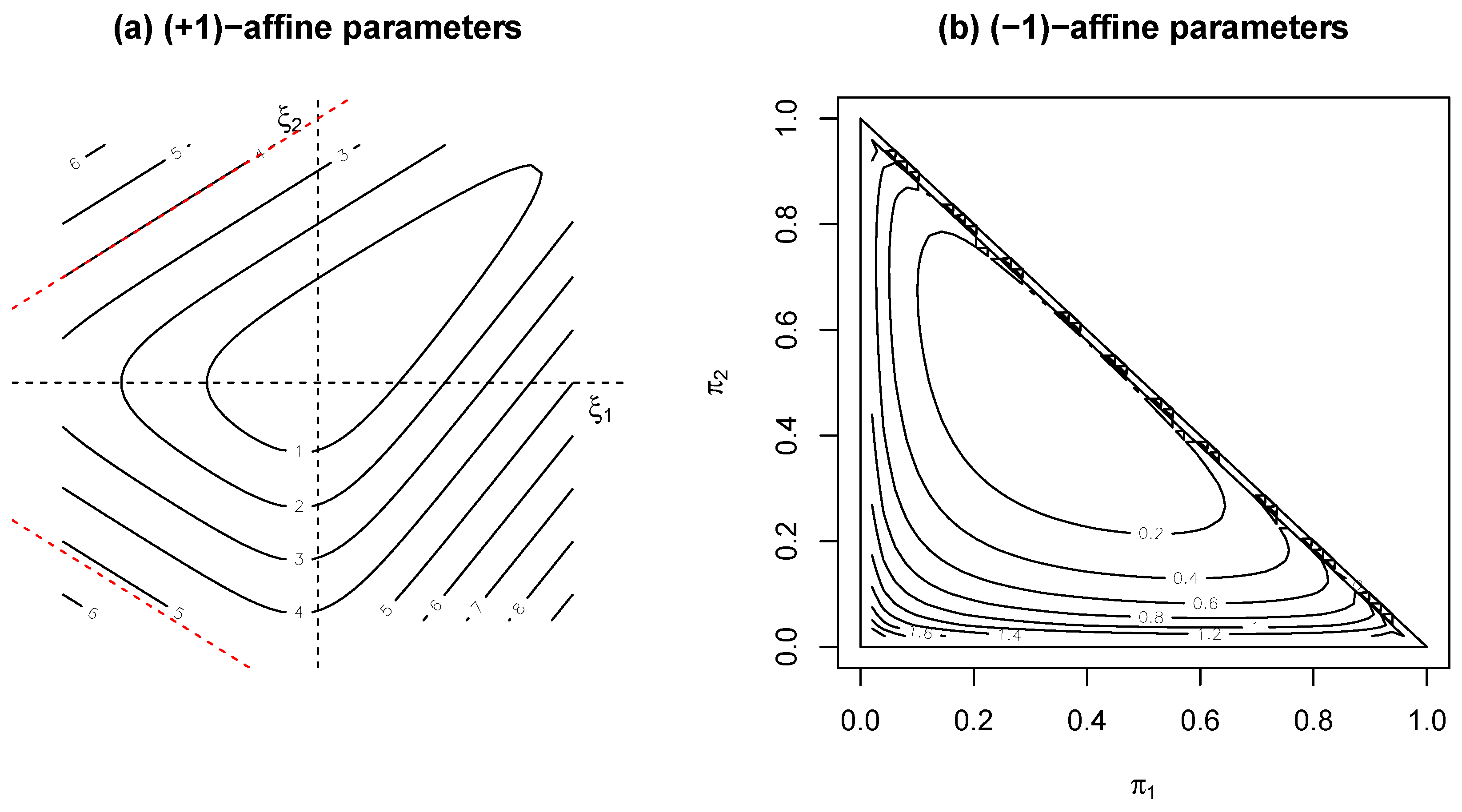
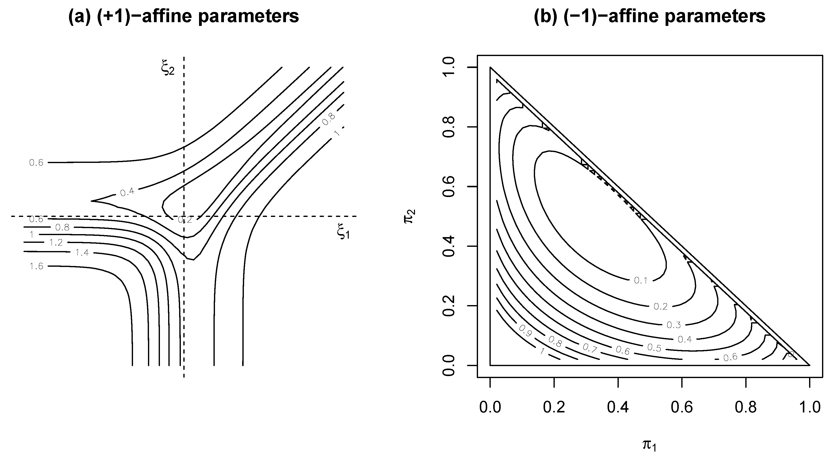
3.3. Links with Information Geometry

At the time that the Power-Divergence family was being examined, there was a parallel development in Information Geometry; oddly, however, it seemed to have taken some time before the links between the two areas were fully recognised. A good treatment of these links can be found in [6] (Chapter 9). Since it is important to understand the extreme values of divergence functions, considerations of convexity can clearly play an important role. The general class of Bregman divergences, [6,34] (page 240), and [35] (page 13) is very useful here. For each Bregman divergence, there will exist affine parameters of the exponential family in which the divergence function is convex. In the class of product Poisson models—which are the key building blocks of log–linear models—all members of the Power-Divergence family have the Bregman property. These are then α-divergences, capable of generating the complete Information Geometry of the model [35], with the link between α and λ given in Table 1. The α-representation highlights the duality properties, which are a cornerstone of Information Geometry, but which is rather hidden in the λ representation. The Bregman divergence representation for the Poisson is given in Table 2. The divergence parameter—in which we have convexity—is shown for each λ, as is the so-called potential function, which generates the complete information geometry for these models.

3.4. Extended Multinomial Case

In this paper, we are focusing on the class of log–linear models where the multinomial is the underlying class of distributions; that is, we condition on the sample size, N, being fixed in the product Poisson space. In particular, we focus on extended multinomials, which includes the closure of the multinomials, so we have a boundary. Due to the conditioning (which induces curvature), only the cases where λ = 0 , 1 remain Bregman divergences, but all are still divergences in the sense of being Csiszár f-divergences [36,37].
The closure of an exponential family (e.g., [11,38,39,40]), and its application in the theory of log–linear models has been explored in [12,13,41,42]. The key here is understanding the limiting behaviour in the natural— α = 1 in the sense of [8]—parameter space. This can be done by considering the polar dual [43], or, alternatively, the directions of recession—[12] or [42]. The boundary polytope determines key statistical properties of the model, including the behaviour of the sampling distribution of (functions of) the MLE and the shape of level sets of divergence functions.
Figure 1 and Figure 2 show level sets of the α = ± 1 Power-Divergences in the ( + 1 ) -affine and ( 1 ) -affine parameters (Panels (a) and (b), respectively) for the k = 2 extended multinomial model. The boundary polytope in this case is a simple triangle “at infinity”, and the shape of this is strongly reflected in the behaviour of the level sets. In Figure 1, we show—in the simplex ( π 0 , π 1 , π 2 ) | i = 0 2 π i = 1 , π i 0 —the level sets of the α = 1 divergence, which, in the Csiszár f-divergence form, is
K ( π 0 , π ) : = i = 0 2 log π i 0 π i π i 0 .
The figures show how in Panel (a), the directions of recession dominate the shape of level sets, and in Panel (b) the duals of these directions (i.e., the vertices of the simplex) each have different maximal behaviour. The lack of convexity of the level sets in Panel (a) corresponds to the fact that the natural parameters are not the affine divergence parameters for this divergence, so we do not expect convex behaviour. In Panel (b), we do get non-convex level sets, as expected.
Figure 2 shows the same story, but this time for the dual divergence,
K * ( π , π 0 ) : = K ( π 0 , π ) .
Now, the affine divergence parameters are shown in Panel (a), the natural parameters. We see that in the limit the shape of the divergence is converging to that of the polar of the boundary polytope. In general, local behaviour is quadratic, but boundary behaviour is polygonal.

4. Simulation Studies

In this section, we undertake simulation studies to numerically explore what has been discussed above. Separate sub-sections address three general topics—focusing on one particular instance of each, as follows:
  • The transition as ( N , k ) varies between discrete and continuous features of the sampling distributions of goodness-of-fit statistics—focusing on the behaviour of the deviance at the uniform discrete distribution;
  • The comparative behaviour of a range of Power-Divergence statistics—focusing on the relative stability of their sampling distributions near the boundary;
  • The lack of uniformity—across the parameter space—of the finite sample adequacy of standard asymptotic sampling distributions, focusing on testing independence in 2 × 2 contingency tables.
For each topic, the results presented invite further investigation.

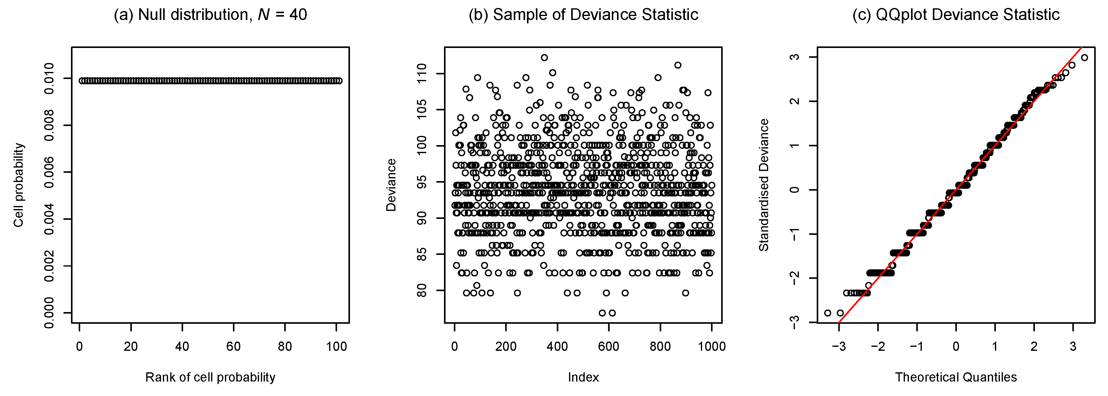
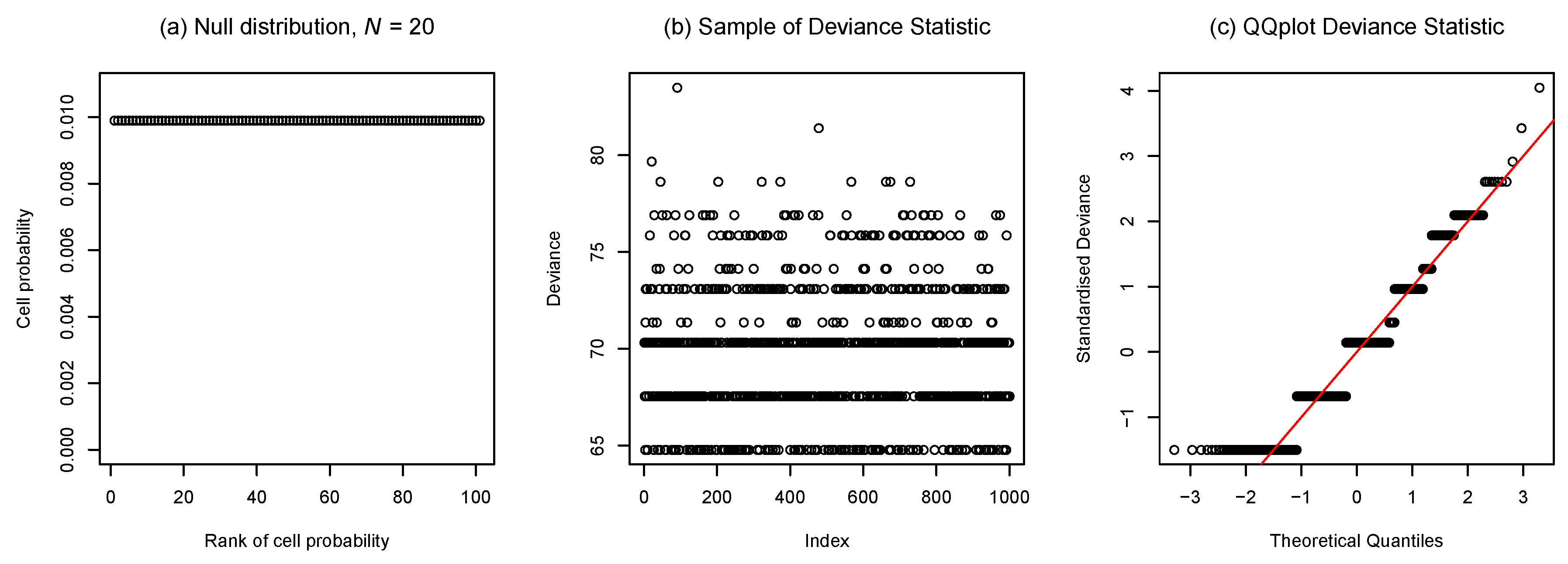
4.1. Transition Between Discrete and Continuous Features of Sampling Distributions

Earlier work [2] used the decomposition:
D * / 2 = { 0 i k : n i * > 0 } n i * log ( n i * / μ i ) = Γ * + Δ * ,
Γ * : = i = 0 k α i n i *   and   Δ * : = { 0 i k : n i * > 1 } n i * log n i * 0 ,   where   α i : = log μ i ,
to show that a particularly bad case for the adequacy of any continuous approximation to the sampling distribution of the deviance D : = D * | ( N * = N ) is the uniform discrete distribution: π i = 1 / ( k + 1 ) . In this case, the Γ * term contributes a constant to the deviance, while the Δ * term has no contributions from cells with 0 or 1 observations—these being in the vast majority in the N < < k situation considered here. In other words, all of the variability in D comes from that between the n i log n i values for the (relatively rare) cell counts above 1. This gives rise to a discreteness phenomenon termed “granularity” in [2], whose meaning was conveyed graphically there in the case N = 30 and k = 200 . Work by Holst [19] predicts that continuous (indeed, normal) approximations will improve with larger values of N / k , as is intuitive. Remarkably, simply doubling the sample size to N = 60 was shown in [2] to be sufficient to give a good enough approximation for most goodness-of-fit testing purposes. In other words, N being 30% of k = 200 was found to be good enough for practical purposes.
Here, we illustrate the role of k-asymptotics (Section 2) in this transition between discrete and continuous features by repeating the above analyses for different values of k. Figure 3 and Figure 4 (where k = 100 while N = 20 and 40, respectively) are qualitatively the same as those presented in [2]. The difference here is that the smaller value of k means that a higher value of N / k (40%) is needed in Figure 4 to adequately remove the granularity evident in Figure 3. For k = 400 , the figures with N = 50 and N = 100 (omitted here for brevity) are, again, qualitatively the same as in [2]—the larger value of k needing only a smaller value of N / k (25%) for practical purposes. Note the QQ-plots used in these two figures are relative to normal quantiles.
The results of this section show the universality of boundary effects. The simulations of Figure 3 and Figure 4 are undertaken under the uniform model, which might be felt to be far from the boundary. In fact, the results show that in the high dimensional, low sample size case, all distributions are “close to” the boundary, and that discretisation effects can dominate.

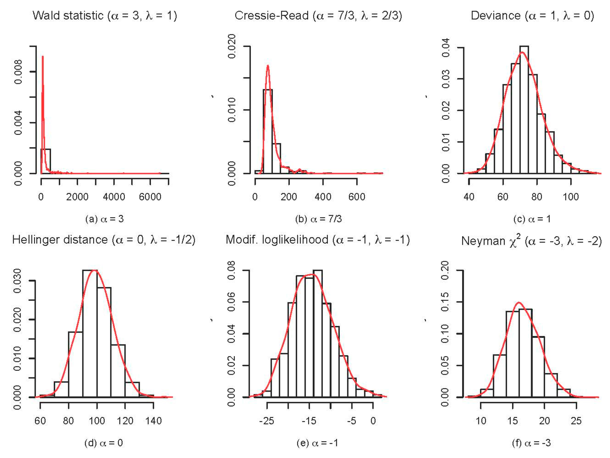
4.2. Comparative Behaviour of Power-Divergence Statistics near the Boundary

Here we study the relative stability—near the boundary of the simplex—of the sampling distributions of a range of Power-Divergence statistics indexed by Amari’s parameter α. Figure 5 shows histograms for six different values of α, N = 50 , k = 200 , and exponentially decreasing values of { π i } , as plotted in Figure 6. In it, red lines depict kernel density estimates using the bandwidth suggested in [44].
These sampling distributions differ markedly. The instability for α = 3 expected from Theorem 1 is clearly visible: very large values contribute to high variance and skewness. Analogous instability features (albeit at a lower level) remain with the Cressie–Read recommended value α = 7 / 3 . In contrast (as expected from the discussion around Theorem 2), the distribution of the deviance ( α = 1 ) is stable and roughly normal. Lower values of α retain these same features.

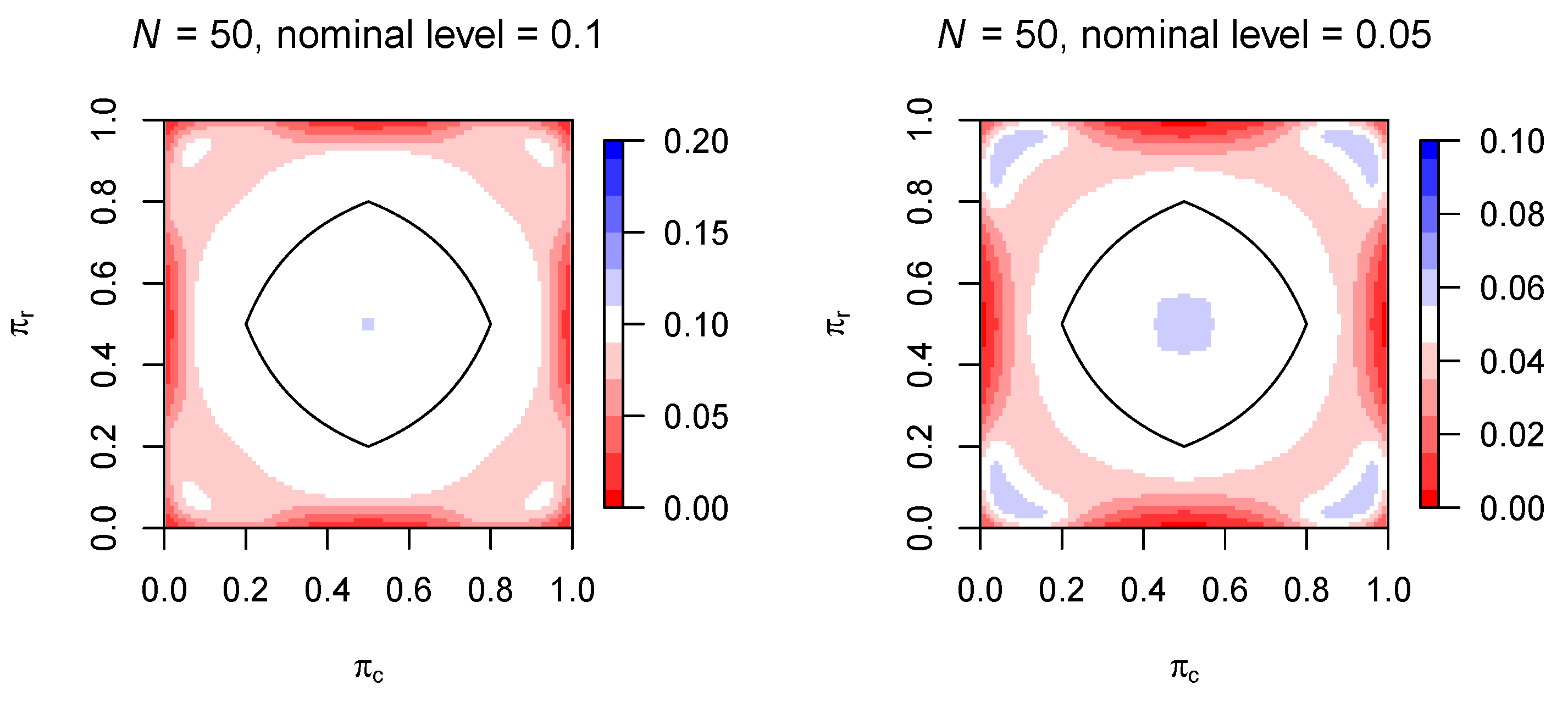
4.3. Variation in Finite Sample Adequacy of Asymptotic Distributions across the Parameter Space

Pearson’s χ 2 statistic ( α = 3 ) is widely used to test independence in contingency tables, a standard rule-of-thumb for its validity being that each expected cell frequency should be at least 5. For illustrative purposes, we consider 2 × 2 contingency tables, the relevant N-asymptotic null distribution being χ 1 2 . We assess the adequacy of this asymptotic approximation by comparing nominal and actual significance levels of this test, based on 10,000 replications. Particular interest lies in how these actual levels vary across different data generation processes within the same null hypothesis of independence.
Figure 7 and Figure 8 show the actual level of the Pearson χ 2 test for nominal levels 0.1 and 0.05 for sample sizes N = 20 and N = 50 , with π r and π c denoting row and column probabilities, respectively. The above general rule applies only at the central black dot in Figure 7, and inside the closed black curved region in Figure 8. The actual level was computed for all pairs of values of π r and π c , averaged using the symmetry of the parameter space, and smoothed using the kernel smoother for irregular 2D data (implemented in the package fields in R). In each case, the white tone contains the nominal level, while red tones correspond to liberal and blue tones to conservative actual levels.
The finite sample adequacy of this standard asymptotic test clearly varies across the parameter space. In particular, its nominal and actual levels agree well at some parameter values outside the standard rule-of-thumb region; and, conversely, disagree somewhat at other parameter values inside it. Intriguingly, the agreement between nominal and actual levels does not improve everywhere with sample size. Overall, the clear patterns evident in this lack of uniformity invite further theoretical investigation.

5. Discussion

This paper has illustrated the key importance of working with the boundary of the closure of exponential families when studying goodness-of-fit testing in the high dimensional, low sample size context. Some of this work is new (Section 2), while some uses the structure of extended exponential families to add insight to standard results in the literature (Section 3). The last section, Section 4, uses simulation studies to start to explore open questions in this area.
One open question—related to the results of Theorems 1 and 2—is to see if a unified theory, for all values of α, and over large classes of extended exponential families, can be developed.

Acknowledgments

The authors would like to thank the EPSRC for the support of grant number EP/L010429/1. Germain Van Bever would also like to thank FRS-FNRS for its support through the grant FC84444. We would also like to thank the referees for very helpful comments.

Author Contributions

All four authors made critical contributions to the paper. R.S. made key contribution to, especially, Section 4. P.M. and F.C. provided the overall structure and key content details of the paper. G.V.B. provided invaluable suggestions throughout.

Conflicts of Interest

The authors declare no conflicts of interest.

Appendix A. Proof of Theorem 1

We start by noting an important recurrence relation which will be exploited in the computations below. By definition, for any t : = ( t i ) R k + 1 , n = ( n i ) has moment generating function
M ( t ; N ) : = E { exp ( t T n ) } = [ m ( t ) ] N
with m ( t ) = i = 0 k a i and a i = a i ( t i ) = π i e t i . Putting
f N , i ( t ; r ) : = N ( r ) m ( t ) N r a i r ( 0 r N ) ,
where
N ( r ) : = N P r = 1 if   r = 0 N ( N 1 ) ( N ( r 1 ) ) if   r { 1 , , N } ,
we have
M ( t ; N ) = f N , i ( t ; 0 ) 0 i k
and the recurrence relation:
f N , i ( t ; r ) t i = f N , i ( t ; r + 1 ) + r f N , i ( t ; r ) 0 i k ; 0 r < N .
When there is no risk of confusion, we may abbreviate M ( t ; N ) to M and f N , i ( t ; r ) to f N ( r ) , or even to f ( r ) —so that (A1) becomes M = f ( 0 ) . Again, we may write r M ( t ; N ) / t i r as M r , r + s M ( t ; N ) / t i r t j s as M r , s and r + s + u M ( t ; N ) / t i r t j s t l u as M r , s , u , with similar conventions for higher order mixed derivatives.
We can now use this to explicitly calculate low order moments of the count vectors. Using E ( n i r ) = r M ( t ; N ) / t i r | t = 0 , the first N moments of n i now follow from (A1) and repeated use of (A2), noting that m ( 0 ) = 1 and a i ( 0 ) = π i .
In particular, the first 6 moments of each n i can be obtained as follows, where N 6 is assumed. Using (A1) and (A2), we have
M 1 = f ( 1 ) M 2 = f ( 2 ) + f ( 1 ) M 3 = f ( 3 ) + 2 f ( 2 ) + f ( 2 ) + f ( 1 ) = f ( 3 ) + 3 f ( 2 ) + f ( 1 ) M 4 = f ( 4 ) + 6 f ( 3 ) + 7 f ( 2 ) + f ( 1 ) M 5 = f ( 5 ) + 10 f ( 4 ) + 25 f ( 3 ) + 15 f ( 2 ) + f ( 1 ) M 6 = f ( 6 ) + 15 f ( 5 ) + 65 f ( 4 ) + 90 f ( 3 ) + 31 f ( 2 ) + f ( 1 ) .
Substituting in, we have
E ( n i ) = N π i E ( n i 2 ) = N ( 2 ) π i 2 + N π i E ( n i 3 ) = N ( 3 ) π i 3 + 3 N ( 2 ) π i 2 + N π i E ( n i 4 ) = N ( 4 ) π i 4 + 6 N ( 3 ) π i 3 + 7 N ( 2 ) π i 2 + N π i E ( n i 5 ) = N ( 5 ) π i 5 + 10 N ( 4 ) π i 4 + 25 N ( 3 ) π i 3 + 15 N ( 2 ) π i 2 + N π i E ( n i 6 ) = N ( 6 ) π i 6 + 15 N ( 5 ) π i 5 + 65 N ( 4 ) π i 4 + 90 N ( 3 ) π i 3 + 31 N ( 2 ) π i 2 + N π i .
This can be formalised in the following Lemma
Lemma A1.
The integer coefficients in any expansion
M r = s = 1 r c r ( s ) f ( s ) ( 1 r N )
can be computed using c r ( 1 ) = c r ( r ) = 1 together, for r 3 , with the update:
c r ( s ) = c r 1 ( s 1 ) + s c r 1 ( s ) ( 1 < s < r ) .
We note that if M r is required for r > N , we may repeatedly differentiate
M N = s = 1 N c N ( s ) f ( s )
w.r.t. t i , noting that f ( N ) = N ! a i N no longer depends on m ( t ) so that, for all h > 0 , h f ( N ) / t i h = N h f ( N ) .
Mixed moments of any order can be derived from those of lower order, exploiting the fact that a i depends on t only via t i . We illustrate this by deriving those required for the second and third moments of W.
First consider the mixed moments required for the second moment of W. Of course, V a r ( W ) = 0 if k = 0 . Otherwise, k > 0 , and computing V a r ( W ) requires E ( n i 2 n j 2 ) for i j . We find this as follows, assuming N 4 .
The relation M 2 = f ( 2 ) + f ( 1 ) established above gives
2 M / t j 2 = N ( 2 ) a j 2 f N 2 ( 0 ) + N a j f N 1 ( 0 ) .
Repeated use of (A3) now gives
M 2 , 2 = N ( 4 ) a i 2 a j 2 f N 4 ( 0 ) + N ( 3 ) a i a j ( a i + a j ) f N 3 ( 0 ) + N ( 2 ) a i a j f N 2 ( 0 )
so that
E ( n i 2 n j 2 ) = N ( 4 ) π i 2 π j 2 + N ( 3 ) π i π j ( π i + π j ) + N ( 2 ) π i π j .
We further look at the mixed moments needed for the third moment of W. For the skewness of W, we need E ( n i 2 n j 4 ) for i j and, when k > 1 , E ( n i 2 n j 2 n l 2 ) for i , j , l distinct. We find these similarly, as follows, assuming k > 1 and N 6 .
Equation (A4) above gives
2 M / t j 2 t l 2 = N ( 4 ) a j 2 a l 2 f N 4 ( 0 ) + N ( 3 ) a j a l ( a j + a l ) f N 3 ( 0 ) + N ( 2 ) a j a l f N 2 ( 0 )
from which, using (A3) repeatedly, we have
M 2 , 2 , 2 = a j 2 a l 2 { N ( 6 ) a i 2 f N 6 ( 0 ) + N ( 5 ) a i f N 5 ( 0 ) } + a j a l ( a j + a l ) { N ( 5 ) a i 2 f N 5 ( 0 ) + N ( 4 ) a i f N 4 ( 0 ) } + a j a l { N ( 4 ) a i 2 f N 4 ( 0 ) + N ( 3 ) a i f N 3 ( 0 ) } = N ( 6 ) a i 2 a j 2 a l 2 f N 6 ( 0 ) + N ( 5 ) a i a j a l { a i a j + a j a l + a l a i } f N 5 ( 0 ) + N ( 4 ) a i a j a l { a i + a j + a l } f N 4 ( 0 ) + N ( 3 ) a i a j a l f N 3 ( 0 )
so that E ( n i 2 n j 2 n l 2 ) equals
N ( 6 ) π i 2 π j 2 π l 2 + N ( 5 ) π i π j π l { π i π j + π j π l + π l π i } + N ( 4 ) π i π j π l { π i + π j + π l } + N ( 3 ) π i π j π l .
Finally, the relation M 4 = f ( 4 ) + 6 f ( 3 ) + 7 f ( 2 ) + f ( 1 ) established above gives
4 M / t j 4 = N ( 4 ) a j 4 f N 4 ( 0 ) + 6 N ( 3 ) a j 3 f N 3 ( 0 ) + 7 N ( 2 ) a j 2 f N 2 ( 0 ) + N a j f N 1 ( 0 )
so that, again using (A3) repeatedly, yields
E ( n i 2 n j 4 ) = N ( 6 ) π i 2 π j 4 + N ( 5 ) π i π j 3 ( 6 π i + π j ) + N ( 4 ) π i π j 2 ( 7 π i + 6 π j ) + N ( 3 ) π i π j ( π i + 7 π j ) + N ( 2 ) π i π j .
Combining above results, we obtain here the first three moments of W. Higher moments may be found similarly.
We first look at E ( W ) . We have W = 1 N 2 i = 0 k n i 2 π i 1 and E ( n i 2 ) = N ( 2 ) π i 2 + N π i , so that
E ( W ) = N ( 2 ) N 2 + ( k + 1 ) N 1 = k N .
The variance is computed by recalling that N 2 ( W + 1 ) = i n i 2 π i , while E ( W ) = k N ,
V a r ( W ) = V a r ( W + 1 ) = A ( 2 ) N 4 k N + 1 2 ,
where
A ( 2 ) : = N 4 E { ( W + 1 ) 2 } = i E ( n i 4 ) π i 2 + i j E ( n i 2 n j 2 ) π i π j .
Using expressions for E ( n i 4 ) and E ( n i 2 n j 2 ) established above, and putting
π ( α ) : = i π i α ,
we have
i E ( n i 4 ) π i 2 = i { N ( 4 ) π i 2 + 6 N ( 3 ) π i + 7 N ( 2 ) + N π i 1 } = N ( 4 ) π ( 2 ) + 6 N ( 3 ) + 7 N ( 2 ) ( k + 1 ) + N π ( 1 )
and
i j E ( n i 2 n j 2 ) π i π j = i j { N ( 4 ) π i π j + N ( 3 ) ( π i + π j ) + N ( 2 ) } = N ( 4 ) ( 1 π ( 2 ) ) + 2 N ( 3 ) k + N ( 2 ) k ( k + 1 ) ,
so that
A ( 2 ) = N ( 4 ) + 2 N ( 3 ) ( k + 3 ) + N ( 2 ) ( k + 1 ) ( k + 7 ) + N π ( 1 ) ,
whence
V a r ( W ) = N ( 4 ) + 2 N ( 3 ) ( k + 3 ) + N ( 2 ) ( k + 1 ) ( k + 7 ) + N π ( 1 ) N 4 1 + k N 2 = π ( 1 ) ( k + 1 ) 2 + 2 k ( N 1 ) N 3 , after some simplification .
Note that V a r ( W ) depends on ( π i ) only via π ( 1 ) while, by strict convexity of x 1 / x ( x > 0 ) ,
π ( 1 ) ( k + 1 ) 2 , equality holding iff π i i 1 / ( k + 1 ) .
Thus, for given k and N, V a r ( W ) is strictly increasing as ( π i ) departs from uniformity, tending to ∞ as one or more π i 0 + .
Finally, for these calculations, we look at E [ W E ( W ) 3 ] . Recalling again that N 2 ( W + 1 ) = i n i 2 π i ,
E [ W E ( W ) 3 ] = E [ ( W + 1 ) E ( W + 1 ) 3 ] = N 6 A ( 3 ) 3 V a r ( W ) ( E ( W ) + 1 ) ( E ( W ) + 1 ) 3 ,
where A ( 3 ) : = N 6 E { ( W + 1 ) 3 } is given by
A ( 3 ) = i E ( n i 6 ) π i 3 + 3 i j E ( n i 2 n j 4 ) π i π j 2 + i , j , l distinct E ( n i 2 n j 2 n l 2 ) π i π j π l .
Given that
E ( W ) = k / N and V a r ( W ) = π ( 1 ) ( k + 1 ) 2 + 2 k ( N 1 ) N 3 ,
it suffices to find A ( 3 ) .
Using expressions for E ( n i 6 ) , E ( n i 2 n j 2 n l 2 ) , and E ( n i 2 n j 4 ) established above, we have
i E ( n i 6 ) π i 3 = N ( 6 ) π ( 3 ) + 15 N ( 5 ) π ( 2 ) + 65 N ( 4 ) + 90 N ( 3 ) ( k + 1 ) + 31 N ( 2 ) π ( 1 ) + N π ( 2 )
i j E ( n i 2 n j 4 ) π i π j 2 = N ( 6 ) π i π j 2 + N ( 5 ) π j ( 6 π i + π j ) + N ( 4 ) ( 7 π i + 6 π j ) + N ( 3 ) ( π i / π j + 7 ) + N ( 2 ) π j 1 = N ( 6 ) { π ( 2 ) π ( 3 ) } + N ( 5 ) { 6 + ( k 6 ) π ( 2 ) } + 13 N ( 4 ) k + N ( 3 ) { π ( 1 ) + ( 7 k 1 ) ( k + 1 ) } + N ( 2 ) k π ( 1 )
and
i , j , l distinct E ( n i 2 n j 2 n l 2 ) π i π j π l = N ( 6 ) { 1 + 2 π ( 3 ) 3 π ( 2 ) } + 3 N ( 5 ) ( k 1 ) { 1 π ( 2 ) } + 3 N ( 4 ) k ( k 1 ) + N ( 3 ) k ( k 2 1 )
so that, after some simplification,
A ( 3 ) = N ( 6 ) + 3 N ( 5 ) ( k + 5 ) + N ( 4 ) { 3 k ( k + 12 ) + 65 } + N ( 3 ) { k 3 + 21 k 2 + 107 k + 87 } + 3 N ( 3 ) π ( 1 ) + N ( 2 ) ( 31 + 3 k ) π ( 1 ) + N π ( 2 ) .
Substituting in and simplifying, we find E [ W E ( W ) 3 ] to be:
π ( 2 ) ( k + 1 ) 3 ( 3 k + 25 22 N ) π ( 1 ) ( k + 1 ) 2 + g ( k , N ) N 5 ,
where
g ( k , N ) = 4 ( N 1 ) k ( k + 2 N 5 ) > 0 .
Note that E [ W E ( W ) 3 ] depends on ( π i ) only via π ( 1 ) and the larger quantity π ( 2 ) . In particular, for given k and N, the skewness of W tends to + as one or more π i 0 + .

Appendix B. Truncate and Bound Approximations

In the notation of Lemma 1, it suffices to find truncate and bound approximations for each of E ( X μ ) , E ( X . X μ ) , and E ( X μ 2 ) .
For all r , s in N , define h r , s ( μ ) : = E { ( log ( X + r ) ) s } . Appropriate choices of m N 0 and a A in (9), together with (10), give:
E ( X μ ) = μ h 1 , 1 ( μ ) μ log μ , E ( X . X μ ) = { μ 2 h 2 , 1 ( μ ) + μ h 1 , 1 ( μ ) } ( μ 2 + μ ) log μ , and : E ( X μ 2 ) = μ 2 h 2 , 2 ( μ ) + μ h 1 , 2 ( μ ) + ( μ 2 + μ ) ( log μ ) 2 2 log μ { μ 2 h 2 , 1 ( μ ) + μ h 1 , 1 ( μ ) } ,
so that it suffices to truncate and bound h r , s ( μ ) for r , s { 1 , 2 } .
For all r , s in N , and for all m N 0 , we write:
h r , s ( μ ) = h r , s [ m ] ( μ ) + ε r , s [ m ] ( μ )
in which:
h r , s [ m ] ( μ ) : = x = 0 m { ( log ( x + r ) ) s } p ( x ) and ε r , s [ m ] ( μ ) : = x = m + 1 { ( log ( x + r ) ) s } p ( x ) .
Using again (7), the “error term” ε r , s [ m ] ( μ ) has lower and upper bounds:
0 < ε r , s [ m ] ( μ ) < ε ¯ r , s [ m ] ( μ ) : = x = m + 1 ( x + ( r 1 ) ) s p ( x ) .
Restricting attention now to r , s { 1 , 2 } , as we may, and requiring m s so that F [ m s ] ( μ ) given by (4) is defined, (8) gives:
ε ¯ 1 , 1 [ m ] ( μ ) = x = m + 1 x p ( x ) = μ x = m p ( x ) = μ { 1 F [ m 1 ] ( μ ) } ,
ε ¯ 2 , 1 [ m ] ( μ ) = x = m + 1 ( x + 1 ) p ( x ) = ε ¯ 1 , 1 [ m ] ( μ ) + { 1 F [ m ] ( μ ) } ,
ε ¯ 1 , 2 [ m ] ( μ ) = x = m + 1 x 2 p ( x ) = x = m + 1 { x ( x 1 ) + x } p ( x ) = μ 2 { 1 F [ m 2 ] ( μ ) } + ε ¯ 1 , 1 [ m ] ( μ )
and:
ε ¯ 2 , 2 [ m ] ( μ ) = x = m + 1 ( x + 1 ) 2 p ( x ) = x = m + 1 { x 2 + ( x + 1 ) + x } p ( x ) = ε ¯ 1 , 2 [ m ] ( μ ) + ε ¯ 2 , 1 [ m ] ( μ ) + ε ¯ 1 , 1 [ m ] ( μ ) .
Accordingly, for given μ, each ε ¯ r , s [ m ] ( μ ) decreases strictly to zero with m providing—to any desired accuracy—truncate and bound approximations for each of ν, τ, and ρ. In this connection, we note that the upper tail probabilities involved here can be bounded by standard Chernoff arguments.

References

  1. Critchley, F.; Marriott, P. Computational Information Geometry in Statistics: Theory and practice. Entropy 2014, 16, 2454–2471. [Google Scholar] [CrossRef]
  2. Marriott, P.; Sabolova, R.; Van Bever, G.; Critchley, F. Geometry of goodness-of-fit testing in high dimensional low sample size modelling. In Geometric Science of Information: Second International Conference, GSI 2015, Palaiseau, France, October 28–30, 2015, Proceedings; Nielsen, F., Barbaresco, F., Eds.; Springer: Berlin, Germany, 2015; pp. 569–576. [Google Scholar]
  3. Amari, S.-I.; Nagaoka, H. Methods of Information Geometry; Translations of Mathematical Monographs; American Mathematical Society: Providence, RI, USA, 2000. [Google Scholar]
  4. Cressie, N.; Read, T.R.C. Multinomial goodness-of-fit tests. J. R. Stat. Soc. B 1984, 46, 440–464. [Google Scholar]
  5. Read, T.R.C.; Cressie, N.A.C. Goodness-of-Fit Statistics for Discrete Multivariate Data; Springer: New York, NY, USA, 1988. [Google Scholar]
  6. Kass, R.E.; Vos, P.W. Geometrical Foundations of Asymptotic Inference; John Wiley & Sons, Inc.: Hoboken, NJ, USA, 1997. [Google Scholar]
  7. Agresti, A. Categorical Data Analysis, 3rd ed.; Wiley: Hoboken, NJ, USA, 2013. [Google Scholar]
  8. Amari, S.-I. Differential-geometrical methods in statistics. In Lecture Notes in Statistics; Springer: New York, NY, USA, 1985; Volume 28. [Google Scholar]
  9. Barndorff-Nielsen, O.E.; Cox, D.R. Asymptotic Techniques for Use in Statistics; Chapman & Hall: London, UK, 1989. [Google Scholar]
  10. Anaya-Izquierdo, K.; Critchley, F.; Marriott, P. When are first-order asymptotics adequate? A diagnostic. STAT 2014, 3, 17–22. [Google Scholar] [CrossRef]
  11. Lauritzen, S.L. Graphical Models; Clarendon Press: Oxford, UK, 1996. [Google Scholar]
  12. Geyer, C.J. Likelihood inference in exponential families and directions of recession. Electron. J. Stat. 2009, 3, 259–289. [Google Scholar] [CrossRef]
  13. Fienberg, S.E.; Rinaldo, A. Maximum likelihood estimation in log-linear models. Ann. Stat. 2012, 40, 996–1023. [Google Scholar] [CrossRef]
  14. Eguchi, S.; Copas, J. Local model uncertainty and incomplete-data bias. J. R. Stat. Soc. B 2005, 67, 1–37. [Google Scholar]
  15. Copas, J.; Eguchi, S. Likelihood for statistically equivalent models. J. R. Stat. Soc. B 2010, 72, 193–217. [Google Scholar] [CrossRef]
  16. Anaya-Izquierdo, K.; Critchley, F.; Marriott, P.; Vos, P. On the geometric interplay between goodness-of-fit and estimation: Illustrative examples. In Computational Information Geometry: For Image and Signal Processing; Lecture Notes in Computer Science (LNCS); Nielsen, F., Dodson, K., Critchley, F., Eds.; Springer: Berlin, Germany, 2016. [Google Scholar]
  17. Morris, C. Central limit theorems for multinomial sums. Ann. Stat. 1975, 3, 165–188. [Google Scholar] [CrossRef]
  18. Osius, G.; Rojek, D. Normal goodness-of-fit tests for multinomial models with large degrees of freedom. JASA 1992, 87, 1145–1152. [Google Scholar] [CrossRef]
  19. Holst, L. Asymptotic normality and efficiency for certain goodness-of-fit tests. Biometrika 1972, 59, 137–145. [Google Scholar] [CrossRef]
  20. Koehler, K.J.; Larntz, K. An empirical investigation of goodness-of-fit statistics for sparse multinomials. JASA 1980, 75, 336–344. [Google Scholar] [CrossRef]
  21. Koehler, K.J. Goodness-of-fit tests for log-linear models in sparse contingency tables. JASA 1986, 81, 483–493. [Google Scholar] [CrossRef]
  22. McCullagh, P. The conditional distribution of goodness-of-fit statistics for discrete data. JASA 1986, 81, 104–107. [Google Scholar] [CrossRef]
  23. Forster, J.J.; McDonald, J.W.; Smith, P.W.F. Monte Carlo exact conditional tests for log-linear and logistic models. J. R. Stat. Soc. B 1996, 58, 445–453. [Google Scholar]
  24. Kim, D.; Agresti, A. Nearly exact tests of conditional independence and marginal homogeneity for sparse contingency tables. Comput. Stat. Data Anal. 1997, 24, 89–104. [Google Scholar] [CrossRef]
  25. Booth, J.G.; Butler, R.W. An importance sampling algorithm for exact conditional tests in log-linear models. Biometrika 1999, 86, 321–332. [Google Scholar] [CrossRef]
  26. Caffo, B.S.; Booth, J.G. Monte Carlo conditional inference for log-linear and logistic models: A survey of current methodology. Stat. Methods Med. Res. 2003, 12, 109–123. [Google Scholar] [CrossRef] [PubMed]
  27. Lloyd, C.J. Computing highly accurate or exact P-values using importance sampling. Comput. Stat. Data Anal. 2012, 56, 1784–1794. [Google Scholar] [CrossRef]
  28. Simonoff, J.S. Jackknifing and bootstrapping goodness-of-fit statistics in sparse multinomials. JASA 1986, 81, 1005–1011. [Google Scholar] [CrossRef]
  29. Gaunt, R.E.; Pickett, A.; Reinert, G. Chi-square approximation by Stein’s method with application to Pearson’s statistic. arXiv, 2015; arXiv:1507.01707. [Google Scholar]
  30. Fan, J.; Hung, H.-N.; Wong, W.-H. Geometric understanding of likelihood ratio statistics. JASA 2000, 95, 836–841. [Google Scholar] [CrossRef]
  31. Ulyanov, V.V.; Zubov, V.N. Refinement on the convergence of one family of goodness-of-fit statistics to chi-squared distribution. Hiroshima Math. J. 2009, 39, 133–161. [Google Scholar]
  32. Asylbekov, Z.A.; Zubov, V.N.; Ulyanov, V.V. On approximating some statistics of goodness-of-fit tests in the case of three-dimensional discrete data. Sib. Math. J. 2011, 52, 571–584. [Google Scholar] [CrossRef]
  33. Zelterman, D. Goodness-of-fit tests for large sparse multinomial distributions. JASA 1987, 82, 624–629. [Google Scholar] [CrossRef]
  34. Bregman, L.M. The relaxation method of finding the common point of convex sets and its application to the solution of problems in convex programming. USSR Comp. Math. Math. 1967, 7, 200–217. [Google Scholar] [CrossRef]
  35. Amari, S.-I. Information Geometry and Its Applications; Springer: Tokyo, Japan, 2015. [Google Scholar]
  36. Csiszár, I. On topological properties of f-divergences. Stud. Sci. Math. Hung. 1967, 2, 329–339. [Google Scholar]
  37. Csiszár, I. Information measures: A critical survey. In Transactions of the Seventh Prague Conference on Information Theory, Statistical Decision Functions, Random Processes and of the 1974 European Meeting of Statisticians; Kozesnik, J., Ed.; Springer: Houten, The Netherlands, 1977; Volume B, pp. 73–86. [Google Scholar]
  38. Barndorff-Nielsen, O. Information and Exponential Families in Statistical Theory; John Wiley & Sons, Ltd.: Chichester, UK, 1978. [Google Scholar]
  39. Brown, L.D. Fundamentals of Statistical Exponential Families with Applications in Statistical Decision Theory; Lecture Notes-Monograph Series; Integrated Media Systems (IMS): Hayward, CA, USA, 1986; Volume 9. [Google Scholar]
  40. Csiszár, I.; Matúš, F. Closures of exponential families. Ann. Probab. 2005, 33, 582–600. [Google Scholar] [CrossRef]
  41. Eriksson, N.; Fienberg, S.E.; Rinaldo, A.; Sullivant, S. Polyhedral conditions for the nonexistence of the MLE for hierarchical log-linear models. J. Symb. Comput. 2006, 41, 222–233. [Google Scholar] [CrossRef]
  42. Rinaldo, A.; Feinberg, S.; Zhou, Y. On the geometry of discrete exponential families with applications to exponential random graph models. Electron. J. Stat. 2009, 3, 446–484. [Google Scholar] [CrossRef]
  43. Critchley, F.; Marriott, P. Computing with Fisher geodesics and extended exponential families. Stat. Comput. 2016, 26, 325–332. [Google Scholar] [CrossRef]
  44. Sheather, S.J.; Jones, M.C. A reliable data-based bandwidth selection method for kernel density estimation. J. R. Stat. Soc. B 1991, 53, 683–690. [Google Scholar]
Figure 1. Level sets of K ( π 0 , π ) , for fixed π 0 = ( 1 6 , 2 6 , 3 6 ) in: (a) the natural parameters, and (b) the mean parameters.
Entropy 18 00421 g001
Figure 2. Level sets of K * ( π 0 , π ) , for fixed π 0 = ( 1 6 , 2 6 , 3 6 ) in: (a) the natural parameters, and (b) the mean parameters.
Entropy 18 00421 g002
Figure 3. k = 100 , N = 20 .
Entropy 18 00421 g003
Figure 4. k = 100 , N = 40 .
Entropy 18 00421 g004
Figure 5. Sampling distributions for six members of the Power-Divergence family.
Entropy 18 00421 g005
Figure 6. Exponentially decreasing values of π i .
Entropy 18 00421 g006
Figure 7. Heatmap of the actual level of the test for N = 20 at nominal levels 0.1 and 0.05; the standard rule-of-thumb (where expected counts are greater than 5) applies only at the black dot.
Entropy 18 00421 g007
Figure 8. Heatmap of the actual level of the test for N = 50 at nominal levels 0.1 and 0.05; the standard rule-of-thumb (where expected counts are greater than 5) applies inside the closed black curved region.
Entropy 18 00421 g008
Table 1. Special cases of the Power-Divergence statistics.
α:= 1+ 2λλFormulaName
31 i = 0 k ( n i N π i ) 2 N π i Pearson χ 2
7/32/3 9 5 i = 0 k n i n i N π i 2 3 1 Read–Cressie
10 2 i = 0 k n i log n i / N π i Twice log-likelihood (deviance)
0 1 2 4 i = 0 k n i N π i 2 Freeman–Tukey or Hellinger
−1−1 2 i = 0 k N π i log N π i / n i Twice modified log-likelihood
−3−2 i = 0 k ( n i N π i ) 2 n i Neyman χ 2
Table 2. Power-Divergence in the Poisson model with mean μ, where λ * = 1 λ .
λαDivergence D λ ( μ 1 , μ 2 ) Divergence Parameter ξPotential
−1−1 μ 1 μ 2 μ 2 log ( μ 1 ) log ( μ 2 ) ξ = log ( μ ) exp ( ξ )
01 μ 2 μ 1 μ 1 log ( μ 2 ) log ( μ 1 ) ξ = μ ξ log ( ξ ) ξ
λ 0 , 1 α ± 1 λ * μ 1 λ * μ 2 μ 2 μ 1 μ 2 λ * 1 λ * ( 1 λ * ) ξ = 1 λ * μ λ * ( λ * ξ ) 1 / λ * 1 λ *

