Non-Asymptotic Confidence Sets for Circular Means ^†

Abstract

The mean of data on the unit circle is defined as the minimizer of the average squared Euclidean distance to the data. Based on Hoeffding’s mass concentration inequalities, non-asymptotic confidence sets for circular means are constructed which are universal in the sense that they require no distributional assumptions. These are then compared with asymptotic confidence sets in simulations and for a real data set.

1. Introduction

In applications, data assuming values on the circle, i.e., circular data, arise frequently, examples being measurements of wind directions, or time of the day that patients are admitted to a hospital unit. We refer to the literature, e.g., [1,2,3,4,5], for an overview of statistical methods for circular data, in particular the ones described in this section.

Here, we will concern ourselves with the arguably simplest statistic, the mean. However, given that a circle does not carry a vector space structure, i.e., there is neither a natural addition of points on the circle nor can one divide them by a natural number, what should the meaning of “mean” be?

In order to simplify the exposition, we specifically consider the unit circle in the complex plane, ${\mathsf{S}}^1=\{z\in \mathbf{C}:|z|=1\}$, and we assume the data can be modelled as independent random variables $Z_1,\cdots ,Z_n$ which are identically distributed as the random variable Z taking values in ${\mathsf{S}}^1$. In the literature, however, the circle is often taken to lie in the real plane ${\mathbf{R}}^2$, i.e., while we denote the point on the circle corresponding to an angle $\theta \in (-\pi ,\pi ]$ by $\exp \left(i\theta \right)=\cos \left(\theta \right)+i\sin \left(\theta \right)\in \mathbf{C}$ one may take it to be $(\cos \theta ,\sin \theta )\in {\mathbf{R}}^2$.

Of course, C is a real vector space, so the Euclidean sample mean ${\overline{Z}}_n=\frac{1}{n}{\sum }_{k=1}^n{Z}_k\in \mathbf{C}$ is well-defined. However, unless all $Z_k$ take identical values, it will (by the strict convexity of the closed unit disc) lie inside the circle, i.e., its modulus $|{\overline{Z}}_n|$ will be less than 1. Though ${\overline{Z}}_n$ cannot be taken as a mean on the circle, if ${\overline{Z}}_n\ne 0$, one might say that it specifies a direction; this leads to the idea of calling ${\overline{Z}}_n/|{\overline{Z}}_n|$ the circular sample mean of the data.

Observing that the Euclidean sample mean is the minimiser of the sum of squared distances, this can be put in the more general framework of Fréchet means [6]: define the set of circular sample means to be

$${\widehat{\mu }}_n=\underset{\zeta \in {\mathsf{S}}^1}{\mathrm{argmin}}\sum _{k=1}^n{|Z_k-\zeta |}^2,$$

(1)

and analoguously define the set of circular population means of the random variable Z to be

$$\mu =\underset{\zeta \in {\mathsf{S}}^1}{\mathrm{argmin}}\mathbf{E}{|Z-\zeta |}^2.$$

(2)

Then, as usual, the circular sample means are the circular population means with respect to the empirical distribution of $Z_1,\cdots ,Z_n$.

The circular population mean can be related to the Euclidean population mean $\mathbf{E} Z$ by noting that ${\mathbf{E}|Z-\zeta |}^2={\mathbf{E}|Z-\mathbf{E}Z|}^2+{|\mathbf{E}Z-\zeta |}^2$ (in statistics, this is called the bias-variance decomposition), so that

$$\mu =\underset{\zeta \in {\mathsf{S}}^1}{\mathrm{argmin}}{|\mathbf{E}Z-\zeta |}^2$$

(3)

is the set of points on the circle closest to $\mathbf{E}Z$. It follows that μ is unique if and only if $\mathbf{E}Z\ne 0$ in which case it is given by $\mu =\mathbf{E}Z/|\mathbf{E}Z|$, the orthogonal projection of $\mathbf{E}Z$ onto the circle; otherwise, i.e., if $\mathbf{E}Z=0$, the set of circular population means is all of ${\mathsf{S}}^1$. We consider the information of whether the circular population mean is not unique, e.g., but not exclusively because Z is uniformly distributed over the circle, to be relevant; it thus should be inferred from the data as well. Analogously, ${\widehat{\mu }}_n$ is either all of ${\mathsf{S}}^1$ or uniquely given by ${\overline{Z}}_n/|{\overline{Z}}_n|$ according to whether ${\overline{Z}}_n$ is 0 or not. Note that ${\overline{Z}}_n\ne 0$ a.s. if Z is continuously distributed on the circle, even if $\mathbf{E}Z=0$. ${\overline{Z}}_n$ is what is known as the vector resultant, while ${\overline{Z}}_n/|{\overline{Z}}_n|$ is sometimes referred to as the mean direction.

The expected squared distances minimised in Equation (2) are given by the metric inherited from the ambient space C; therefore, μ is also called the set of extrinsic population means. If we measured distances intrinsically along the circle, i.e., using arc-length instead of chordal distance, we would obtain what is called the set of intrinsic population means. We will not consider the latter in the following, see e.g., [7] for a comparison and [8,9] for generalizations of these concepts.

Our aim is to construct confidence sets for the circular population mean μ that form a superset of μ with a certain (so-called) coverage probability that is required to be not less than some pre-specified significance level $1-\alpha$ for $\alpha \in (0,1)$.

The classical approach is to construct an asymptotic confidence interval where the coverage probability converges to $1-\alpha$ when n tends to infinity. This can be done as follows: since Z is a bounded random variable, $\sqrt{n}({\overline{Z}}_n-\mathbf{E}Z)$ converges to a bivariate normal distribution when identifying C with ${\mathbf{R}}^2$. Now, assume $\mathbf{E}Z\ne 0$ so μ is unique. Then, the orthogonal projection is differentiable in a neighbourhood of $\mathbf{E}Z$, so the δ-method (see e.g., [1] (p. 111) or [4] (Lemma 3.1)) can be applied and one easily obtains

$$\sqrt{n}\mathbf{Arg}\left({\mu }^{-1}{\widehat{\mu }}_n\right)\stackrel{\mathcal{D}}{\to }\mathcal{N}\left(0,\frac{\mathbf{E}{\left(\mathbf{Im}\left({\mu }^{-1}Z\right)\right)}^2}{{|\mathbf{E}Z|}^2}\right),$$

(4)

where $\mathbf{Arg}:\mathbf{C}\backslash \left\{0\right\}\to (-\pi ,\pi ]\subset \mathbf{R}$ denotes the argument of a complex number (it is defined arbitrarily at $0\in \mathbf{C}$), while multiplying with ${\mu }^{-1}$ rotates such that $\mathbf{E}Z=\mu$ is mapped to $0\in (-\pi ,\pi ]$, see e.g., [4] (Proposition 3.1) or [7] (Theorem 5). Estimating the asymptotic variance and applying Slutsky’s lemma, one arrives at the asymptotic confidence set $C_A=\{\zeta \in {\mathsf{S}}^1:|\mathbf{Arg}\left({\zeta }^{-1}{\widehat{\mu }}_n\right)|<{\delta }_A\}$ provided ${\widehat{\mu }}_n$ is unique, where the angle determining the interval is given by

$${\delta }_A=\frac{q_{1-\frac{\alpha }{2}}}{n|{\overline{Z}}_n|}\sqrt{\sum _{k=1}^n{(\mathbf{Im}({\widehat{\mu }}_n^{-1}{Z}_k))}^2},$$

(5)

with $q_{1-\frac{\alpha }{2}}$ denoting the $(1-\frac{\alpha }{2})$-quantile of the standard normal distribution $\mathcal{N}(0,1)$.

There are two major drawbacks to the use of asymptotic confidence intervals: firstly, by definition, they do not guarantee a coverage probability of at least $1-\alpha$ for finite n, so the coverage probability for a fixed distribution and sample size may be much smaller. Indeed, Simulation 2 in Section 4 demonstrates that, even for $n=100$, the coverage probability may be as low as $64\%$ when constructing the asymptotic confidence set for $1-\alpha =90\%$. Secondly, they assume that $\mathbf{E}Z\ne 0$, so they are not applicable to all distributions on the circle. Since in practice it is unknown whether this assumption hold, one would have to test the hypothesis $\mathbf{E}Z=0$, possibly again by an asymptotic test, and construct the confidence set conditioned on this hypothesis having been rejected, setting $C_A={\mathsf{S}}^1$ otherwise. However, this sequential procedure would require some adaptation taking the pre-test into account (cf. e.g., [10])—we come back to this point in Section 5—and it is not commonly implemented in practice.

We therefore aim to construct non-asymptotic confidence sets for μ, guaranteeing coverage with at least the desired probability for any sample size n, which in addition are universal in the sense that they do not make any distributional assumptions about the circular data besides them being independent and identically distributed. It has been shown in [7] that this is possible; however, the confidence sets that were constructed there were far too large to be of use in practice. Nonetheless, we start by varying that construction in Section 2 but using Hoeffding’s inequality instead of Chebyshev’s as in [7]. Considerable improvements are possible if one takes the variance $\mathbf{E}{(\mathbf{Im}({\mu }^{-1}Z))}^2$ “perpendicular to $\mathbf{E}Z$” into account; this is achieved by a second construction in Section 3. Of course, the latter confidence sets will still be conservative but Proposition 2(iv) shows that they are (for $1-\alpha =95\%$) only a factor $\sim \frac{3}{2}$ longer than the asymptotic ones when the sample size n is large. We further illustrate and compare those confidence sets in simulations and for an application to real data in Section 4, discussing the results obtained in Section 5.

2. Construction Using Hoeffding’s Inequality

We will construct a confidence set as the acceptance region of a series of tests. This idea has been used before for the construction of confidence sets for the circular population mean [7] (Section 6); however, we will modify that construction by replacing Chebyshev’s inequality—which is too conservative here—by three applications of Hoeffding’s inequality [11] (Theorem 1): if $U_1,\cdots ,U_n$ are independent random variables taking values in the bounded interval $[a,b]$ with $-\infty <a<b<\infty .$ Then, ${\overline{U}}_n=\frac{1}{n}{\sum }_{k=1}^n{U}_k$ with $\mathbf{E}{\overline{U}}_n=\nu$ fulfills

$$\mathbf{P}\left({\overline{U}}_n-\nu \ge t\right)\le {\left[{\left(\frac{\nu -a}{\nu -a+t}\right)}^{\nu -a+t}{\left(\frac{b-\nu }{b-\nu -t}\right)}^{b-\nu -t}\right]}^{\frac{n}{b-a}}$$

(6)

for any $t\in (0,b-\nu )$. The bound on the right-hand side—denoted $\beta \left(t\right)$—is continuous and strictly decreasing in t (as expected; see Appendix A) with $\beta \left(0\right)=1$ and ${\lim }_{t\to b-\nu }\beta \left(t\right)={\left(\frac{\nu -a}{b-a}\right)}^n$ whence a unique solution $t=t(\gamma ,\nu ,a,b)$ to the equation $\beta \left(t\right)=\gamma$ exists for any $\gamma \in \left({\left(\frac{\nu -a}{b-a}\right)}^n,1\right)$. Equivalently, $t(\gamma ,\nu ,a,b)$ is strictly decreasing in $\gamma .$ Furthermore, $\nu +t(\gamma ,\nu ,a,b)$ is strictly increasing in ν (see Appendix A again), which is also to be expected. While there is no closed form expression for $t(\gamma ,\nu ,a,b)$, it can without difficulty be determined numerically.

Note that the estimate

$$\beta \left(t\right)\le \exp \left(-2n{t}^2/{(b-a)}^2\right)$$

(7)

is often used and called Hoeffding’s inequality [11]. While this would allow to solve explicitly for t, we prefer to work with β as it is sharper, especially for ν close to b as well as for large t. Nonetheless, it shows that the tail bound $\beta \left(t\right)$ tends to zero as fast as if using the central limit theorem which is why it is widely applied for bounded variables, see e.g., [12].

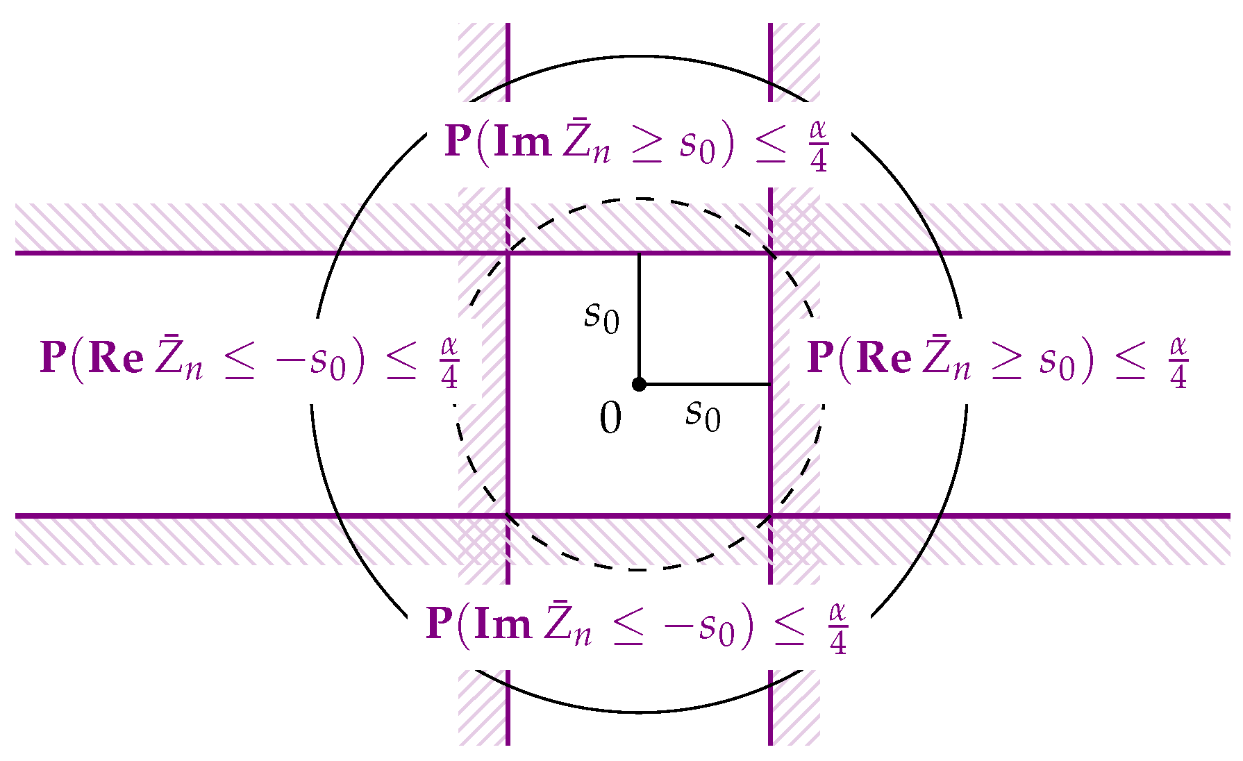
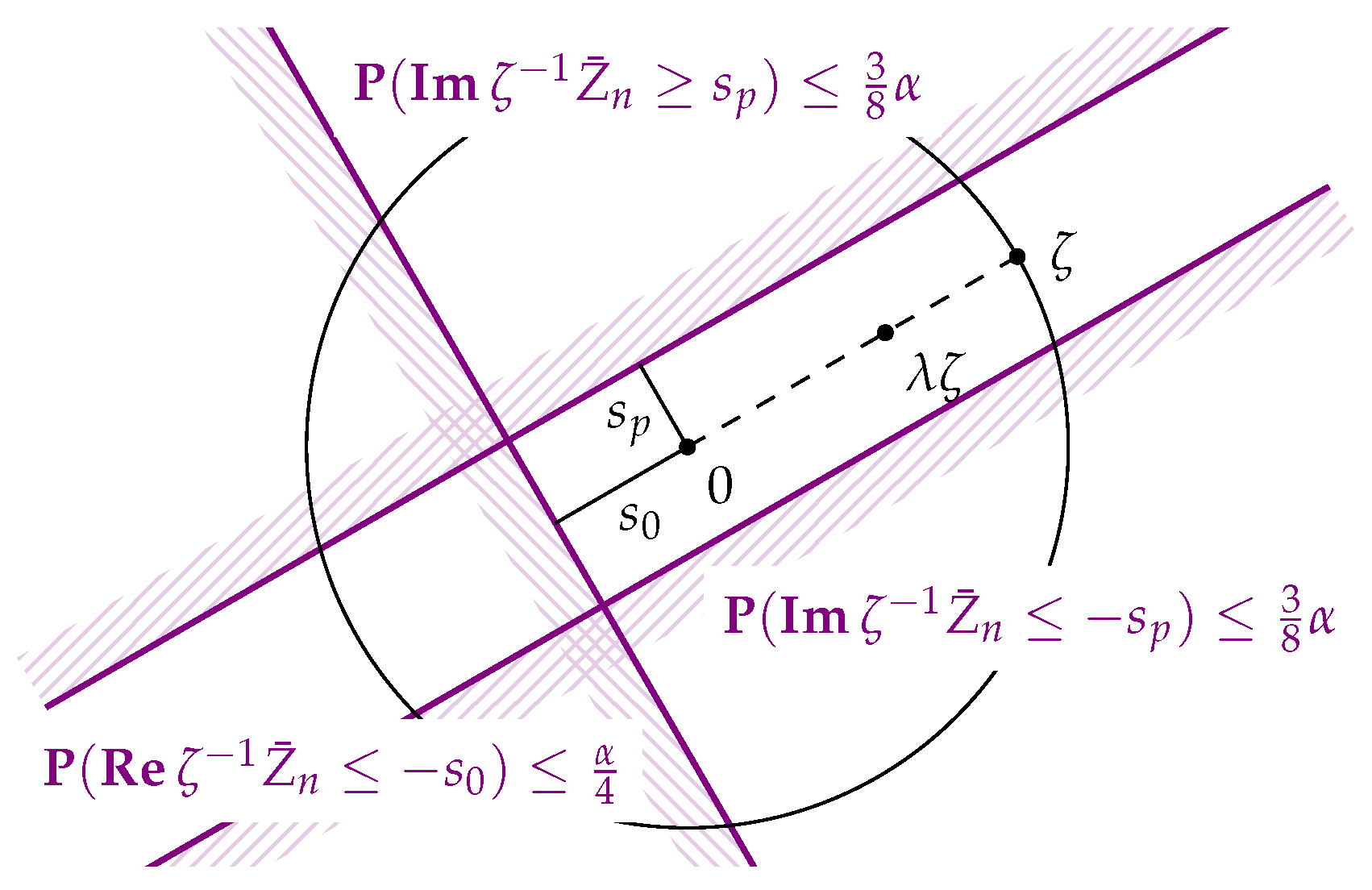
Now, for any $\zeta \in {\mathsf{S}}^1$, we will test the hypothesis that ζ is a circular population mean. This hypothesis is equivalent to saying that there is some $\lambda \in [0,1]$ such that $\mathbf{E}Z=\lambda \zeta$. Multiplication by ${\zeta }^{-1}$ then rotates $\mathbf{E}Z$ onto the non-negative real axis: $\mathbf{E}{\zeta }^{-1}Z=\lambda \ge 0$.

Now, fix ζ and consider $X_k=\mathbf{Re}\left({\zeta }^{-1}{Z}_k\right)$, $Y_k=\mathbf{Im}\left({\zeta }^{-1}{Z}_k\right)$ for $k=1,\cdots ,n$ which may be viewed as the projection of $Z_1,\cdots ,Z_k$ onto the line in the direction of ζ and onto the line perpendicular to it. Both are sequences of independent random variables taking values in $[-1,1]$ with $\mathbf{E}{X}_k=\lambda$ and $\mathbf{E}{Y}_k=0$ under the hypothesis. They thus fulfill the conditions for Hoeffding’s inequality with $a=-1$, $b=1$ and $\nu =\lambda$ or 0, respectively.

We will first consider the case of non-uniqueness of the circular mean, i.e., $\mu ={\mathsf{S}}^1$, or equivalently $\lambda =0$. Then, the critical value $s_0=t(\frac{\alpha }{4},0,-1,1)$ is well-defined for any $\frac{\alpha }{4}>2^{-n},$ and we get $\mathbf{P}({\overline{X}}_n\ge s_0)\le \frac{\alpha }{4}$, and also, by considering $-X_1,\cdots ,-X_n$, that $\mathbf{P}(-{\overline{X}}_n\ge s_0)\le \frac{\alpha }{4}$. Analogously, $\mathbf{P}(|{\overline{Y}}_n|\ge s_0)\le 2\frac{\alpha }{4}=\frac{\alpha }{2}$. We conclude that

$$\mathbf{P}\left(|{\overline{Z}}_n|\ge \sqrt{2}{s}_0\right)=\mathbf{P}\left(|{\overline{X}}_n{|}^2+{|{\overline{Y}}_n|}^2\ge 2s_0^2\right)\le \mathbf{P}\left(|{\overline{X}}_n{|}^2\ge s_0^2\right)+\mathbf{P}\left(|{\overline{Y}}_n{|}^2\ge s_0^2\right)\le \alpha .$$

Rejecting the hypothesis $\mu ={\mathsf{S}}^1$, i.e., $\mathbf{E}Z=0$, if $|{\overline{Z}}_n|\ge \sqrt{2}{s}_0$ thus leads to a test whose probability of false rejection is at most α (see Figure 1). Of course, one may work with $|{\overline{X}}_n{|}^2\ge s_0^2$ and $|{\overline{Y}}_n{|}^2\ge s_0^2$ as criterions for rejection; however, we prefer working with $|{\overline{Z}}_n|\ge \sqrt{2}{s}_0$ since it is independent of the chosen $\zeta .$

Figure 1. The construction for the test of the hypothesis $\mu ={\mathsf{S}}^1,$ or equivalently $\mathbf{E}Z=0.$

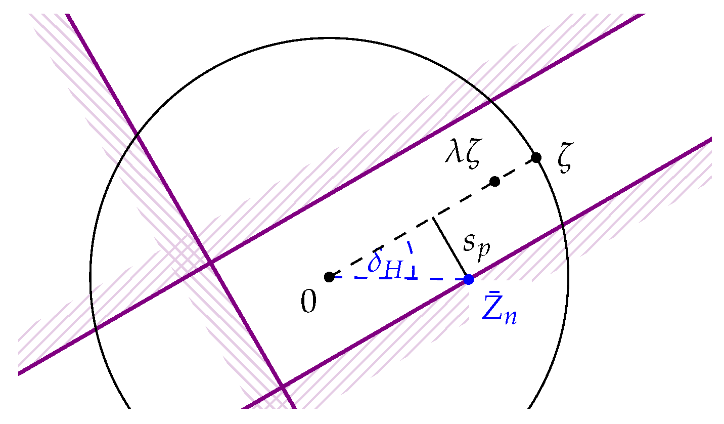
In the case of uniqueness of the circular mean, i.e., for the hypothesis $\lambda >0$, we use the monotonicity of $\nu +t(\gamma ,\nu ,a,b)$ in ν and obtain

$$\mathbf{P}\left({\overline{X}}_n\le -s_0\right)=\mathbf{P}\left(-{\overline{X}}_n\ge t(\frac{\alpha }{4},0,-1,1)\right)\le \mathbf{P}\left(-{\overline{X}}_n\ge -\lambda +t(\frac{\alpha }{4},-\lambda ,-1,1)\right)\le \frac{\alpha }{4}$$

as well. For the direction perpendicular to the direction of ζ (see Figure 2), however, we may now work with $\frac{3}{8}\alpha$, so for $s_p=t(\frac{3}{8}\alpha ,0,-1,1)$—which is well-defined whenever $s_0$ is since $\frac{3}{8}\alpha >\frac{\alpha }{4}>2^{-n}$—we obtain

$$\mathbf{P}({\overline{Y}}_n\ge s_p)+\mathbf{P}\left({\overline{Y}}_n\le -s_p\right)\le 2·\frac{3}{8}\alpha .$$

Rejecting if ${\overline{X}}_n\le -s_0$ or $|{\overline{Y}}_n|\ge s_p$, then, will happen with probability at most $\frac{\alpha }{4}+2·\frac{3}{8}\alpha =\alpha$ under the hypothesis $\mu =\zeta$. In case that we already rejected the hypothesis $\mu ={\mathsf{S}}^1$, i.e., if $|{\overline{Z}}_n|\ge \sqrt{2}{s}_0$, ζ will not be rejected if and only if ${\overline{X}}_n>s_0>0$ and $|{\overline{Y}}_n|<s_p<s_0$ which is then equivalent to $|\mathbf{Arg}\left({\zeta }^{-1}{\overline{Z}}_n\right)|=\arcsin (|{\overline{Y}}_n|/|{\overline{Z}}_n|)<\arcsin (s_p/|{\overline{Z}}_n|)={\delta }_H$ (see Figure 3).

Figure 2. The construction for the test of the hypothesis $\mathbf{E}Z=\lambda \zeta$ with $\lambda >0$.

Figure 3. The critical ${\overline{Z}}_n$ regarding the rejection of ζ. ${\delta }_H$ bounds the angle between ${\widehat{\mu }}_n$ and any accepted $\zeta .$

Define $C_H$ as all ζ which we could not reject, i.e.,

$$C_H=\left\{\begin{array}{cc}{\mathsf{S}}^1,\hfill & \mathrm{if} \alpha \le 2^{-n+2} \mathrm{or} |{\overline{Z}}_n|\le \sqrt{2}{s}_0,\hfill \\ \left\{\zeta \in {\mathsf{S}}^1:|\mathbf{Arg}\left({\zeta }^{-1}{\widehat{\mu }}_n\right)|<{\delta }_H\right\}\hfill & \mathrm{otherwise}.\hfill \end{array}\right.$$

(8)

Then, we obtain the following result:

Proposition 1.

Let $Z_1,\cdots ,Z_n$ be random variables taking values on the unit circle ${\mathsf{S}}^1,$ $\alpha \in (0,1)$, and let $C_H$ be defined as in Equation (8).

(i) 

$C_H$ is a $(1-\alpha )$-confidence set for the circular population mean set. In particular, if $\mathbf{E}Z=0$, i.e., the circular population mean set equals ${\mathsf{S}}^1$, then $|{\overline{Z}}_n|>\sqrt{2}{s}_0$ with probability at most $\alpha ,$ so indeed $C_H={\mathsf{S}}^1$ with probability at least $1-\alpha .$

(ii) 

$s_0$ and $s_p$ are of order $n^{-\frac{1}{2}}$.

(iii) 

If $\mathbf{E}Z\ne 0,$ then $\sqrt{n}{\delta }_H\to 0$ in probability and the probability of obtaining the trivial confidence set, i.e., $\mathbf{P}(C_H={\mathsf{S}}^1)=\mathbf{P}(|{\overline{Z}}_n|\le \sqrt{2}{s}_0)$, goes to 0 exponentially fast.

Proof. 

(i) holds by construction.

For (ii), recall Equation (7), from which we obtain the estimates $\frac{\alpha }{4}\le \exp (-n{s}_0^2/2)$ resp. $\frac{3}{8}\alpha \le \exp (-n{s}_p^2/2)$, implying that $s_0$ and $s_p$ are of order $n^{-\frac{1}{2}};$ the same holds stochastically for ${\delta }_H$ since ${\overline{Z}}_n\to \mathbf{E}Z$ a.s. Regarding the second statement of (iii), if μ is unique, consider $\zeta =-\mu$; then, $\tau =\mathbf{E}{\overline{X}}_n<0$ and $-\sqrt{2}{s}_0$ is eventually less than $\frac{\tau }{2}$ and also $\alpha >2^{-n+2}$ eventually. Hence, the probability of obtaining the trivial confidence set $C_H={\mathsf{S}}^1$ is eventually bounded by $\mathbf{P}(\zeta \in C_H)\le \mathbf{P}({\overline{X}}_n>-s_0)\le \mathbf{P}({\overline{X}}_n>\frac{\tau }{2})=\mathbf{P}({\overline{X}}_n-\mathbf{E}{\overline{X}}_n>-\frac{\tau }{2})\le \exp (-n{\tau }^2/8)$, and thus will go to zero exponentially fast as n tends to infinity. ☐

3. Estimating the Variance

From the central limit theorem for ${\widehat{\mu }}_n$ in case of unique μ, cf. Equation (4), we see that the aymptotic variance of ${\widehat{\mu }}_n$ gets small if $|\mathbf{E}Z|$ is close to 1 (then $\mathbf{E}Z$ is close to the boundary ${\mathsf{S}}^1$ of the unit disc, which is possible only if the distribution is very concentrated) or if the variance $\mathbf{E}{\left(\mathbf{Im}\left({\mu }^{-1}Z\right)\right)}^2$ in the direction perpendicular to μ is small (if the distribution were concentrated on $\pm \mu$, this variance would be zero and ${\widehat{\mu }}_n$ would equal μ with large probability). While ${\delta }_H$ ($|{\overline{Z}}_n|$ being the denominator of its sine) takes the former into account, the latter has not been exploited yet. To do so, we need to estimate $\mathbf{E}{\left(\mathbf{Im}\left({\mu }^{-1}Z\right)\right)}^2$.

Consider $V_n=\frac{1}{n}{\sum }_{k=1}^n{Y}_k^2$ that is under the hypothesis that the corresponding ζ is the unique circular population mean has expectation ${\sigma }^2=\mathbf{Var}\left(Y_k\right)=\mathbf{E}{\left(\mathbf{Im}\left({\zeta }^{-1}Z\right)\right)}^2$. Now, $1-V_n=\frac{1}{n}{\sum }_{k=1}^n(1-Y_k^2)$ is the mean of n independent random variables taking values in $[0,1]$ and having expectation $1-{\sigma }^2$. By another application of Equation (6), we obtain $\mathbf{P}({\sigma }^2\ge V_n+t)=\mathbf{P}(1-V_n\ge 1-{\sigma }^2+t)\le \frac{\alpha }{4}$ for $t=t(\frac{\alpha }{4},1-{\sigma }^2,0,1)$, the latter existing if $\frac{\alpha }{4}>{(1-{\sigma }^2)}^n$. Since $1-{\sigma }^2+t(\frac{\alpha }{4},1-{\sigma }^2,0,1)$ increases with $1-{\sigma }^2$, there is a minimal ${\sigma }^2$ for which $1-V_n\ge 1-{\sigma }^2+t(\frac{\alpha }{4},1-{\sigma }^2,0,1)$ holds and becomes an equality; we denote it by $\widehat{{\sigma }^2}=V_n+t(\frac{\alpha }{4},1-\widehat{{\sigma }^2},0,1)$. Inserting into Equation (6), it by construction fulfills

$$\frac{\alpha }{4}={\left[{\left(\frac{1-\widehat{{\sigma }^2}}{1-V_n}\right)}^{1-V_n}{\left(\frac{\widehat{{\sigma }^2}}{V_n}\right)}^{V_n}\right]}^n.$$

(9)

It is easy to see that the right-hand side depends continuously on and is strictly decreasing in $\widehat{{\sigma }^2}\in [V_n,1]$ (see Appendix A), thereby traversing the interval $[0,1]$ so that one can again solve the equation numerically. We then may, with an error probability of at most $\frac{\alpha }{4}$, use $\widehat{{\sigma }^2}$ as an upper bound for ${\sigma }^2$. Note that $\widehat{{\sigma }^2}>V_n$ exists if $\frac{\alpha }{4}>{(1-\widehat{{\sigma }^2})}^n.$ The latter is fulfilled for any $V_n<1$ since Equation (9) is equivalent to

$$\frac{\alpha }{4}={(1-\widehat{{\sigma }^2})}^n{\left[\underset{>1}{\underbrace{\left(\frac{1}{1-V_n}\right)}}\underset{>1}{\underbrace{{\left(\frac{1-\widehat{{\sigma }^2}}{1-V_n}\right)}^{-V_n}}}\underset{>1}{\underbrace{{\left(\frac{\widehat{{\sigma }^2}}{V_n}\right)}^{V_n}}}\right]}^n.$$

For $V_n=1$, let $\widehat{{\sigma }^2}=1$ be the trivial bound.

With such an upper bound on its variance, we now can get a better estimate for $\mathbf{P}({\overline{Y}}_n>t)$. Indeed, one may use another inequality by Hoeffding [11] (Theorem 3): the mean ${\overline{W}}_n=\frac{1}{n}{\sum }_{k=1}^n{W}_k$ of a sequence $W_1,\cdots ,W_n$ of independent random variables taking values in $(-\infty ,1]$, each having zero expectation as well as variance ${\rho }^2$ fulfills

$$\begin{array}{cc}\hfill \mathbf{P}\left({\overline{W}}_n\ge w\right)& \le {\left[{\left(1+\frac{w}{{\rho }^2}\right)}^{-{\rho }^2-w}{\left(1-w\right)}^{w-1}\right]}^{\frac{n}{1+{\rho }^2}},\hfill \end{array}$$

(10)

$$\begin{array}{cc}\hfill & \le \exp (-nt[(1+\frac{{\rho }^2}{t})\ln (1+\frac{t}{{\rho }^2})-1]).\hfill \end{array}$$

(11)

for any $w\in (0,1).$ Again, an elementary calculation (analogous to Lemma A1) shows that the right-hand side of Equation (10) is strictly decreasing in w, continuously ranging between 1 and ${(\frac{{\rho }^2}{1+{\rho }^2})}^n$ as w varies in $(0,1)$, so that there exists a unique $w=w(\gamma ,{\rho }^2)$ for which the right-hand side equals γ, provided $\gamma \in \left({(\frac{{\rho }^2}{1+{\rho }^2})}^n,1\right)$. Moreover, the right-hand side increases with ${\rho }^2$ (as expected), so that $w(\gamma ,{\rho }^2)$ is increasing in ${\rho }^2$, too (cf. Appendix A).

Therefore, under the hypothesis that the corresponding ζ is the unique circular population mean, $\mathbf{P}\left(|{\overline{Y}}_n|\ge w(\frac{\alpha }{4},{\sigma }^2)\right)\le 2\frac{\alpha }{4}=\frac{\alpha }{2}$. Now, since $\mathbf{P}(w(\frac{\alpha }{4},{\sigma }^2)\ge w(\frac{\alpha }{4},\widehat{{\sigma }^2}))=\mathbf{P}({\sigma }^2\ge \widehat{{\sigma }^2})\le \frac{\alpha }{4}$, setting $s_V=w(\frac{\alpha }{4},\widehat{{\sigma }^2})$ we get $\mathbf{P}\left(|{\overline{Y}}_n|\ge s_V\right)\le \frac{3}{4}\alpha$. Note that $\frac{{\rho }^2}{1+{\rho }^2}$ increases with ${\rho }^2$, so in case $s_0$ exists, $\widehat{{\sigma }^2}\le 1$ implies $\frac{\alpha }{4}>2^{-n}\ge {\left(\frac{\widehat{{\sigma }^2}}{1+\widehat{{\sigma }^2}}\right)}^n$, i.e., the existence of $s_V$.

Following the construction for $C_H$ from Section 2, we can again obtain a confidence set for μ with coverage probability at least $1-\alpha$ as shown in our previous article [13]. In practice however, this confidence set is hard to calculate since $\widehat{{\sigma }^2}=\widehat{{\sigma }^2}\left(\zeta \right)$ has to be calculated for every $\zeta \in {\mathsf{S}}^1.$ Though these confidence sets can be approximated by using a grid as in [13], we suggest using a simultaneous upper bound for the variance of $\mathbf{Im}{\zeta }^{-1}{Z}_k$.

We obtain a (conservative) connected, symmetric confidence set $C_V\subseteq C_H$ by testing $\zeta \in C_H$ with $\widehat{{\sigma }_{\max }^2}={\sup }_{\zeta \in C_H}\widehat{{\sigma }^2}$ as a common upper bound for the variance perpendicular to any $\zeta \in C_H$. Note that $\widehat{{\sigma }_{\max }^2}$ can be obtained as the solution of Equation (9) with

$${\tilde{V}}_n=\underset{\zeta \in C_H}{\sup }\frac{1}{n}\sum _{k=1}^n{\left(\mathbf{Im}{\zeta }^{-1}{Z}_k\right)}^2.$$

Furthermore, we can shorten $C_V$ by iteratively redefining ${\tilde{V}}_n={\sup }_{\zeta \in C_V}\frac{1}{n}{\sum }_{k=1}^n{\left(\mathbf{Im}{\zeta }^{-1}{Z}_k\right)}^2$ and recalculating $C_V$ (see Algorithm 1). The resulting opening angle will be denoted by ${\delta }_V=\arcsin \frac{s_V}{|{\overline{Z}}_n|}.$

Algorithm 1: Algorithm for computation of $C_V$.

Proposition 2.

Let $Z_1,\cdots ,Z_n$ be random variables taking values on the unit circle ${\mathsf{S}}^1,$ and let $\alpha \in (0,1).$

(i) 

The set $C_V$ resulting from Algorithm 1 is a $(1-\alpha )$-confidence set for the circular population mean set. In particular, if $\mathbf{E}Z=0$, i.e., the circular population mean set equals ${\mathsf{S}}^1$, then $|{\overline{Z}}_n|>\sqrt{2}{s}_0$ with probability at most $\alpha ,$ so indeed $C_V={\mathsf{S}}^1$ with probability of at least $1-\alpha .$

(ii) 

$s_V$ is of order $n^{-\frac{1}{2}}$.

(iii) 

If $\mathbf{E}Z\ne 0,$ i.e., if the circular population mean is unique, then $\sqrt{n}{\delta }_V\to 0$ in probability, and the probability of obtaining a trivial confidence set, i.e., $\mathbf{P}(C_H={\mathsf{S}}^1)=\mathbf{P}(|{\overline{Z}}_n|\le \sqrt{2}{s}_0)$, goes to 0 exponentially fast.

(iv) 

If $\mathbf{E}Z\ne 0$, then

$$\underset{n\to \infty }{\mathrm{lim\; sup}}\frac{{\delta }_V}{{\delta }_A}\le \frac{\sqrt{-2\ln \frac{\alpha }{4}}}{q_{1-\frac{\alpha }{2}}}a.s.$$

with $q_{1-\frac{\alpha }{2}}$ denoting the $(1-\frac{\alpha }{2})$-quantile of the standard normal distribution $\mathcal{N}(0,1).$

Proof. 

Again, (i) follows by construction, while (iii) is shown as in Proposition 1.

For (ii), note that $s_V\le s_0$ since the bound in Equation (10) for ${\rho }^2=1$ agrees with the bound in Equation (6) for $a=-1,$ $b=1$ and $v=0,$ thus $s_V$ and ${\delta }_V$ are at least of the order $n^{-\frac{1}{2}}.$

For (iv), we will use the estimate in Equation (11). Recall that $\ln (1+x)=x-\frac{x^2}{2}+o(x^2)$; therefore, for large n and hence small $s_V$ a.s.

$$\begin{array}{cc}\hfill \frac{\alpha }{4}& \le \exp \left(-n{s}_V\left[\left(1+\frac{\widehat{{\sigma }_{\max }^2}}{s_V}\right)\left(\frac{s_V}{\widehat{{\sigma }_{\max }^2}}-\frac{s_V^2}{2{(\widehat{{\sigma }_{\max }^2})}^2}+o\left(s_V^2\right)\right)-1\right]\right)\hfill \\ & =\exp (-n{s}_V^2/2\widehat{{\sigma }_{\max }^2}+o(s_V^2)),\hfill \end{array}$$

thus $s_V\le \sqrt{-2\widehat{{\sigma }_{\max }^2}\ln (\frac{\alpha }{4})/n}+o(n^{-\frac{1}{2}}).$ Additionally, $\arcsin x=x+o\left(x\right)$ for x close to 0 which gives ${\delta }_V=s_V/|{\overline{Z}}_n|+o(s_V)\le \sqrt{-2\widehat{{\sigma }_{\max }^2}\ln \frac{\alpha }{4}}/(\sqrt{n}|{\overline{Z}}_n|)+o(n^{-\frac{1}{2}})$ a.s.

Furthermore, $\widehat{{\sigma }_{\max }^2}\to {\sigma }^2$ a.s. for $n\to \infty$, and we obtain

$$\underset{n\to \infty }{\mathrm{lim\; sup}}\frac{{\delta }_V}{{\delta }_A}\le \frac{\sqrt{-2\ln \frac{\alpha }{4}}}{q_{1-\frac{\alpha }{2}}}\mathrm{a}.\mathrm{s}.$$

since

$${\delta }_A=\frac{q_{1-\frac{\alpha }{2}}}{\sqrt{n}|{\overline{Z}}_n|}\underset{\to \sqrt{{\sigma }^2}}{\underbrace{\sqrt{\frac{1}{n}\sum _{k=1}^n{(\mathbf{Im}({\widehat{\mu }}_n^{-1}{Z}_k))}^2}}}$$

(see Equation (5)). ☐

4. Simulation and Application to Real Data

We will compare the asymptotic confidence set $C_A$, the confidence set $C_H$ constructed directly using Hoeffding’s inequality in Section 2, and the confidence set $C_V$ resulting from Algorithm 1 by reporting their corresponding opening angles ${\delta }_A$, ${\delta }_H$, and ${\delta }_V$ in degrees (${}^{\circ }$) as well as their coverage frequencies in simulations.

All computations have been performed using our own code based on the software package R (version 2.15.3) [14] .

4.1. Simulation 1: Two Points of Equal Mass at $\pm {10}^{\circ }$

First, we consider a rather favourable situation: $n=400$ independent draws from the distribution with $\mathbf{P}(Z=\exp (10\pi i/180))=\mathbf{P}(Z=\exp (-10\pi i/180))=\frac{1}{2}$. Then, we have $|\mathbf{E}Z|=\mathbf{E}Z=\cos (10\pi i/180)\approx 0.985$, implying that the data are highly concentrated, $\mu =1$ is unique, and the variance of Z in the direction of μ is 0; there is only variation perpendicular to μ, i.e., in the direction of the imaginary axis (see Figure 4).

Figure 4. Two points of equal mass at $\pm {10}^{\circ }$ and their Euclidean mean.

Table 1 shows the results based on 10,000 repetitions for a nominal coverage probability of $1-\alpha =95\%$: the average ${\delta }_H$ is about $3.5$ times larger than ${\delta }_V$, which is about twice as large as ${\delta }_A$. As expected, the asymptotics are rather precise in this situation: $C_A$ did cover the true mean in about $95\%$ of the cases, which implies that the other confidence sets are quite conservative; indeed $C_H$ and $C_V$ covered the true mean in all repetitions. One may also note that the angles varied only a little between repetitions.

Table 1. Results for simulation 1 (two points of equal mass at $\pm {10}^{\circ }$) based on 10,000 repetitions with $n=400$ observations each: average observed ${\delta }_H$, ${\delta }_V$, and ${\delta }_A$ (with corresponding standard deviation), as well as frequency (with corresponding standard error) with which $\mu =1$ was covered by $C_H$, $C_V$, and $C_A$, respectively; the nominal coverage probability was $1-\alpha =95\%$.

Confidence Set	Mean δ (±s.d.)	Coverage Frequency (±s.e.)
$C_H$	${8.2}^{\circ }$ ($\pm {0.0005}^{\circ }$)	$100.0\%$ ($\pm 0.0\%$)
$C_V$	${2.4}^{\circ }$ ($\pm {0.0025}^{\circ }$)	$100.0\%$ ($\pm 0.0\%$)
$C_A$	${1.0}^{\circ }$ ($\pm {0.0019}^{\circ }$)	$94.8\%$ ($\pm 0.2\%$)

4.2. Simulation 2: Three Points Placed Asymmetrically

Secondly, we consider a situation which has been designed to show that even a considerably large sample size ($n=100$) does not guarantee approximate coverage for the asymptotic confidence set $C_A$: the distribution of Z is concentrated on three points, ${\xi }_j=\exp ({\theta }_j\pi i/180)$, $j=1,2,3$ with weights ${\omega }_j=\mathbf{P}(Z={\xi }_j)$ chosen such that $\mathbf{E}Z=|\mathbf{E}Z|=0.9$ (implying a small variance and $\mu =1$), ${\omega }_1=1\%$ and $\mathbf{Arg}{\xi }_1>0$, while $\mathbf{Arg}{\xi }_2,\mathbf{Arg}{\xi }_3<0$. In numbers, ${\theta }_1\approx 25.8$, ${\theta }_2\approx -0.3$, and ${\theta }_3\approx -179.7$ (in ${}^{\circ }$) while ${\omega }_2\approx 94\%$, and ${\omega }_3\approx 5\%$ (see Figure 5).

Figure 5. Three points placed asymmetrically with different masses and their Euclidean mean.

The results based on 10,000 repetitions are shown in Table 2 where a nominal coverage probability of $1-\alpha =90\%$ was prescribed. Clearly, $C_A$ with its coverage probability of less than $64\%$ performs quite poorly while the others are conservative; ${\delta }_V\approx 5^{\circ }$ still appears small enough to be useful in practice, though.

Table 2. Results for simulation 2 (three points placed asymmetrically) based on 10,000 repetitions with $n=100$ observations each: average observed ${\delta }_H$, ${\delta }_V$, and ${\delta }_A$ (with corresponding standard deviation), as well as frequency (with corresponding standard error) with which $\mu =1$ was covered by $C_H$, $C_V$, and $C_A$, respectively; the nominal coverage probability was $1-\alpha =90\%$.

Confidence Set	Mean δ (±s.d.)	Coverage Frequency (±s.e.)
$C_H$	${16.5}^{\circ }$ ($\pm {0.85}^{\circ }$)	$100.0\%$ ($\pm 0.0\%$)
$C_V$	${5.0}^{\circ }$ ($\pm {0.38}^{\circ }$)	$100.0\%$ ($\pm 0.0\%$)
$C_A$	${0.4}^{\circ }$ ($\pm {0.28}^{\circ }$)	$62.8\%$ ($\pm 0.5\%$)

4.3. Real Data: Movements of Ants

Fisher [3] (Example 4.4) describes a data set of the directions 100 ants took in response to an illuminated target placed at ${180}^{\circ }$ for which it may be of interest to know whether the ants indeed (on average) move towards that target (see [15] for the original publication). The data set is available as Ants_radians within the R package CircNNTSR [16].

The circular sample mean for this data set is about $-{176.9}^{\circ }$; for a nominal coverage probability of $1-\alpha =95\%$, one gets ${\delta }_H\approx {27.3}^{\circ }$, ${\delta }_V\approx {20.5}^{\circ }$, and ${\delta }_A\approx {9.6}^{\circ }$ so that all confidence sets contain $\pm {180}^{\circ }$ (see Figure 6). The data set’s concentration is not very high, however, so the circular population mean could—according to $C_V$—also be $-{156.4}^{\circ }$ or ${162.6}^{\circ }$.

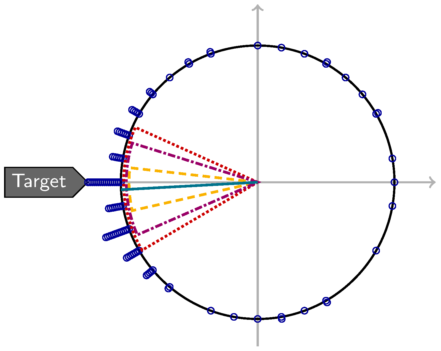
Figure 6. Ant data ( ) placed at increasing radii to visually resolve ties; in addition, the circular mean direction ( ) as well as confidence sets $C_H$ ( ), $C_V$ ( ), and $C_A$ ( ) are shown.

5. Discussion

We have derived two confidence sets, $C_H$ and $C_V$, for the set of circular sample means. Both guarantee coverage for any finite sample size without making any assumptions on the distribution of the data (besides that they are independent and identically distributed) at the cost of potentially being quite conservative; they are non-asymptotic and universal in this sense. Judging from the simulations and the real data set, $C_V$—which estimates the variance perpendicular to the mean direction—appears to be preferable over $C_H$ (as expected) and small enough to be useful in practice.

While the asymptotic confidence set’s opening angle is less than half (asymptotically about $2/3$ for $\alpha =5\%$) of the one for $C_V$ in our simulations and application, it has the drawback that even for a sample size of $n=100$, it may fail to give a coverage probability close to the nominal one; in addition, one has to assume that the circular population mean is unique. Of course, one could also devise an asymptotically justified test for the latter but this would entail a correction for multiple testing (for example working with $\frac{\alpha }{2}$ each time), which would also render the asymptotic confidence set conservative.

Further improvements would require sharper “universal” mass concentration inequalities taking the first or the first two moments into account; however, this is beyond the scope of this article.