Boltzmann Complexity: An Emergent Property of the Majorization Partial Order

Abstract

Boltzmann macrostates, which are in 1:1 correspondence with the partitions of integers, are investigated. Integer partitions, unlike entropy, uniquely characterize Boltzmann states, but their use has been limited. Integer partitions are well known to be partially ordered by majorization. It is less well known that this partial order is fundamentally equivalent to the “mixedness” of the set of microstates that comprise each macrostate. Thus, integer partitions represent the fundamental property of the mixing character of Boltzmann states. The standard definition of incomparability in partial orders is applied to the individual Boltzmann macrostates to determine the number of other macrostates with which it is incomparable. We apply this definition to each partition (or macrostate) and calculate the number C with which that partition is incomparable. We show that the value of C complements the value of the Boltzmann entropy, S, obtained in the usual way. Results for C and S are obtained for Boltzmann states comprised of up to $N=50$ microstates where there are 204,226 Boltzmann macrostates. We note that, unlike mixedness, neither C nor S uniquely characterizes macrostates. Plots of C vs. S are shown. The results are surprising and support the authors’ earlier suggestion that C be regarded as the complexity of the Boltzmann states. From this we propose that complexity may generally arise from incomparability in other systems as well.

1. Introduction to Integer Partitions and Their Relation to Boltzmann States

The Boltzmann equation, $S=kln\mathrm{\Omega }$, is generally the first statistical model of entropy treated in introductory chemistry textbooks. Its fundamental contribution is the connection of entropy, S, with the statistical probability, Ω, of the occurrence of accessible states of the system [1]. Here k is Boltzmann’s constant.

Consider a macrostate of a Boltzmann system of N distinguishable particles distributed among N states with ${\lambda }_k$ particles in state k. The number of ways this macrostate can arise is simply the number of ways N–distinguishable particles can be distributed in N boxes, namely

$$\mathrm{\Omega }=\frac{N!}{{\prod }_{k=1}^N{\lambda }_k!}$$

(1)

The sum of all accessible macrostates is then

$$\mathrm{\Xi }(N,V,E)=\sum _{\mathrm{\Omega }}\mathrm{\Omega }$$

(2)

We note that the number of macrostates, Ξ, obtained combinatorially via (2), is involved in all statistical ensembles [1]. For a macrostate with N microstates and with ${\lambda }_1$ particles of type 1, ${\lambda }_2$ particles of type 2, etc., we can uniquely identify the macrostate with the “integer partition” of N $[\lambda ]=[{\lambda }_1,{\lambda }_2,{\lambda }_3,\dots ,{\lambda }_N]$ with ${\lambda }_i\ge 0$ and $\mathrm{\Sigma }\left({\lambda }_i\right)=N$. In general, we can take ${\lambda }_i\ge {\lambda }_j$ when $i<j$.

The problem of calculating the number of integer partitions as a function of N has been widely studied, and that number is found to grow exponentially with the square root of N [2]. For N larger than 50 this becomes a very large number, with over 200,000 partitions of the number 50, and more than 3 trillion partitions if $N=200$. Integer partitions have a long history in group theory. Young represented the partitions by diagrams consisting of rows of boxes, with the top row having ${\lambda }_1$ boxes, the second having ${\lambda }_2$ boxes, etc. [3]. Using these diagrams, mathematicians were able to develop formulas for the dimensions of the irreducible representations of the symmetric group $S_N$ (See Rutherford’s monograph [4]). Moshinsky [5] also related the Young diagrams to the Gelfand states of the unitary group $U_N$.

2. The Mixing Partial Order

In general, a set of objects X (in our case, partitions) can be organized in many ways. Some organizational schemes result in a unique order for the members of the set, while others only partially order the members. A unique order was given by Young [6] for Boltzmann states, which has had, to our knowledge, no physical or statistical application. Here we consider the mixing partial order, which is consistent with increasing Boltzmann entropy $S_{[\lambda ]}/k=$ ln ${\omega }_{[\lambda ]}$ obtained from (1).

We have previously observed [7] that there is a high degree of degeneracy among the Boltzmann states with respect to $S_{[\lambda ]}$, so that while $S_{[\lambda ]}$ is a scalar, the Boltzmann states are only partially ordered by entropy. In other words, states that have the same value of $S_{[\lambda ]}$ cannot be uniquely compared or ordered by entropy. Of course, other more general partial orders are possible if one considers the compete vector (or diagram) corresponding to the partition itself. Investigations of such partial orders are rarely found in the chemical/physics literature.

In 1903, Muirhead [8] introduced a partial order for partitions that has a long history in combinatorics. To define this partial order, let $\lambda =[{\lambda }_1,{\lambda }_2,\dots ,{\lambda }_N]$ be a partition of N. The criterion of majorization (or dominance) is that a partition λ majorizes another partition μ (symbolized $\lambda \succ \mu$) if and only if

$$\sum _{i=1}^m{\lambda }_i\ge \sum _{i=1}^m{\mu }_i\forall m=1\mathrm{to}N$$

(3)

Over a half century later, Ruch [9] revisited the majorization partial order in the chemical literature with respect to Boltzmann statistics. According his classic paper, “When we classify a set of N objects according to some principle, we obtain a subdivision into subsets without objects in common. Independently of the nature of the classification principle, we can represent the subsets by a diagram, if, for example, we consider the rows as representing the numbers of equivalent objects [9].” This diagram is the Young diagram [4]. Further, he proved that the majorization partial order is mathematically equivalent to the partial order of any set of objects by how mixed the set is.

Mixedness is a fundamental property. However, because it is a partial order rather than a scalar it is not frequently discussed. Thus, an example of the mixing concept might be useful. Consider a set of six distinguishable objects, for example, fruits. For simplicity we could label them a,b,c,d,e and f. First we note that the subsets {a,a,a,a,b,b} and {d,d,d,d,e,e} have the same mixing character, namely $[4,2]$. In other words, a basket with 4 plums and 2 oranges has the same mixing character as one with 4 peaches and 2 melons. The most mixed basket, then, has six different fruits in it and is represented as the partition $[1,1,1,1,1,1]$ or $[1^6]$. Similarly, the least mixed is a basket containing 6 of the same fruit and is represented by $[N]$. Next consider the subsets {a,a,a,a,b,c} and {a,a,a,a,b,b} corresponding to the partitions $[4,1,1]$ and $[4,2]$ respectively. Now $[4,1,1]$ is more mixed than $[4,2]$ if it can be formed by combining baskets of type $[4,2]$. To show this, mix two subsets {a,a,a,a,b,b} with two {a,a,a,a,c,c}; both have mixing character $[4,2]$. This leads to a combined set with 16 a’s, 4 b’s and 4 c’s. However, that is equivalent to 4 sets, each of which have the mixing character $[4,1,1]$. In a similar manner one can show that $[3,2,1]$ is more mixed than both $[4,2]$ and $[4,1,1]$. However, the question of whether $[4,1,1]$ is more or less mixed than $[3,3]$ cannot be answered because neither can be obtained via mixtures of the other. Mathematically they are incomparably mixed. It is this mixing partial order that Ruch proved to be exactly equivalent to the majorization partial order of integer partitions. The first occurrence of incomparability occurs when $N=6$, but for larger N incomparability becomes more and more important as discussed below.

Recently, renewed attention has been given to majorization; this is largely the result of its importance in quantum entanglement and quantum computing. Our purpose here, however, is to investigate a property of Boltzmann macrostates that emerges from the majorization partial order, namely complexity. If the set of objects is the set of all Boltzmann states, the relationship to mixing provides a link to Boltzmann statistics and led Ruch to suggest a generalization of the second law of thermodynamics in isolated systems, namely that “the time development of a statistical (Gibbs-) ensemble of isolated systems (microcanonical ensemble) proceeds in such a way that the mixing character increases [9].”

It is frequently useful to depict partial orders as lattices or diagrams. Particularly useful is the Hasse diagram [10] for the majorization partial order for partitions where one represents each partition as a vertex in the plane and draws a line segment or curve that goes upward from μ to λ whenever λ majorizes μ (that is, whenever $\lambda \succ \mu$ and there is no ρ such that $\lambda \succ \rho \succ \mu$). For integer partitions, this diagram is often referred to as the Young Diagram Lattice (YDL). Figure 1 shows the Hasse diagram or YDL for the majorization partial order for Boltzmann macrostates composed of 10 microstates each.

3. Incomparability in Partial Orders

While this paper will focus on majorization, many of the ideas apply to partially ordered sets (sometimes called posets) in general [11,12,13]. The most striking feature associated with many posets is that while some members of the set are comparable under the order relation, others are fundamentally incomparable. For example, if the set is the set of integer partitions, two partitions are incomparable under majorization if neither majorizes the other according to (3). In this section, we discuss the general concept of incomparability in any partial order and define the incomparability number for members of the poset. Partial orderings of a set X can be represented as $\mathbf{P}=(X,P)$ where P is the partial order relation [13]. If X is the set of integer partitions, $IP$—the three partial orders discussed above, namely Young’s order, entropy, and majorization—would be $\mathbf{Y}=(IP,Young)$, $\mathbf{S}=(IP,entropy)$, and $\mathbf{M}=(IP,majorization)$.

Consider a general set X with partial order $\mathbf{P}$. For each $x_i\in$ X, we define the scalar $C_{\mathbf{P}}\left(x_i\right)$ as the number of elements of X with which it is incomparable under the order relation P. A mathematically related scalar, $A_{\mathbf{P}}\left(x_i\right)$ is defined as the number of elements of X that are mutually incomparable to $x_i$ under the order relation P. This set is termed an antichain containing $x_i$. In 2006, Seitz suggested that the complexity of an element $x_i\in$ X under a partial order relation is the length of the maximal antichain that contains $x_i$ [14]. Later, Seitz and Kirwan [15] suggested that $C_{\mathbf{P}}\left(x_i\right)$ is a more easily obtained quantitative complexity measure for $x_i$. Clearly, both $\mathbf{C}$ and $\mathbf{A}$ can only be defined with respect to the underlying partial order $\mathbf{P}$.

The concept of incomparability developed above applies to all partially ordered sets. In the next section we will compute the incomparability for the mixing partial order $\mathbf{M}$ of the Boltzmann states. The results will lead us to propose the following:

Proposition. 

The complexity of a Boltzmann state $[\lambda ]=[{\lambda }_1,{\lambda }_2,{\lambda }_3,\dots ,{\lambda }_N]$, is given by its incomparability number $C_{\mathbf{M}}\left([\lambda ]\right)$, and consequently complexity is an emergent property of the majorization partial order.

4. Finite N Results

In this section, we present finite N results. For $N=10$ there are 42 partitions, and the Hasse diagram was easily drawn (see Figure 1). As discussed above, many partitions are incomparable to one another. For example, in Figure 1, the 12 red partitions are incomparable to the partition [6,1,1,1,1] shown in blue; hence $C_{\mathbf{M}}\left([6,1,1,1,1]\right)=12$. A similar analysis for all partitions $[\lambda ]$ gives $C_{\mathbf{M}}\left([\lambda ]\right)$. The problem of obtaining $C_{\mathbf{M}}\left([\lambda ]\right)$ for $N=50$ was solved numerically for the 204,226 Boltzmann states by exhaustive application of the majorization condition in (3) to each state. A plot of entropy normalized by the equilibrium entropy vs. $C_{\mathbf{M}}\left([\lambda ]\right)$ for $N=50$ is shown in Figure 2.

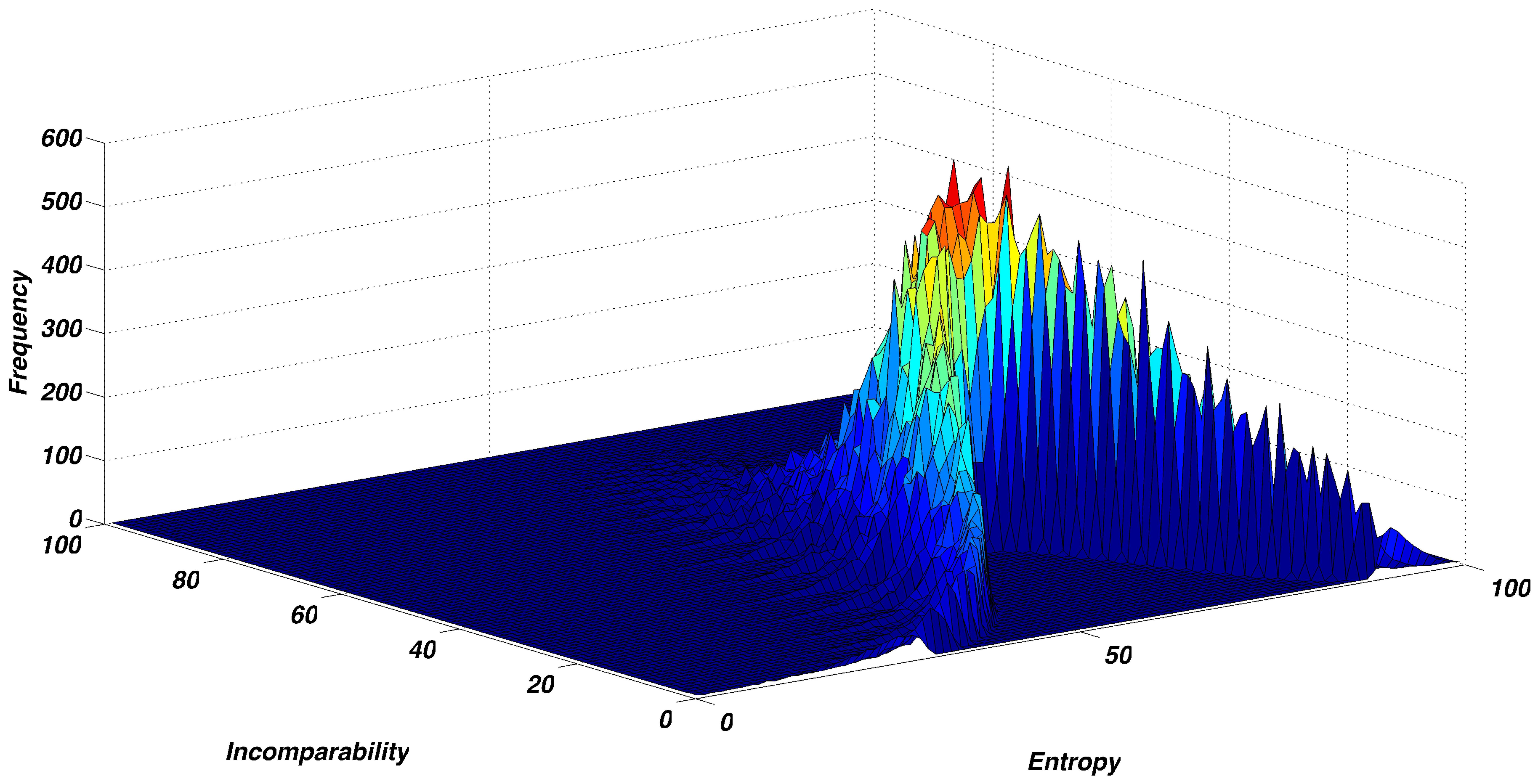
For $N=50$ with over 200,000 states, it is possible to look at the density of macrostates as a function of normalized entropy and C. Figure 3 shows the results obtained by overlaying a $100\times 100$ grid on Figure 2 and counting the number of states in each grid section. Figure 4 shows the same results where the density is assigned to a third dimension.

The finite N results in Figure 2, Figure 3 and Figure 4 were obtained without approximation or assumptions regarding dynamics. The results are, therefore, entirely computational and present what we believe is an entirely new way to characterize Boltzmann states namely by their fundamental nature as partitions with two complementary views: entropy (related to disorder) and incomparability (related to complexity). The results are both surprising and beautiful.

Three features of Figure 2 stand out. First is the treelike appearance. The branches represent states with greatly different entropies having the same or very similar incomparability. If we examine the outermost points (those of maximum incomparability at each entropy) we find that these are for states with partitions $[N-m,1^m]$. Thus at low entropy, the first partition to show significant incomparability is $[49,1]$. Moving to the next outermost point we find the partition $[48,1^2]$ etc. This trend continues until the maximum incomparability is obtained at $[N/2,1^{N/2}]$. In Figure 1, this sequence of partitions occurs on the far right of the YDL. The second feature is the asymmetry. Given that the maximum incomparability occurs at $[N/2,1^{N/2}]$ we use Stirling’s approximation for the normalized entropy at that state to give

$$\overline{S}[N/2,1^{N/2}]=\frac{S[N/2,1^{N/2}]}{S[1^N]}\approx \left(\frac{1}{2}\right)\left[1+\left(\frac{ln2}{lnN-1}\right)\right]$$

(4)

Clearly this approaches $0.5$ as $N\to \infty$. However, the convergence is slow. For $N=50$ $\overline{S}=0.619015$, while for Avagadro’s number $\overline{S}=0.50645$. It would seem then that in most applications the incomparability peak will be shifted toward the equilbrium entropy and so the fall in incomparability will be faster than the rise. A related consequence of this asymmetry is shorter incomparability branches. The third feature is the “desert” of “simple” (i.e., low incomparability) states at mid entropy. All states in this region have significant complexity. For $N=10$, if one considers Figure 1, one notes that this YDL (with 42 partitions) increases in “width” as entropy/mixing increases until reaching a maximum at mid entropy. Extrapolating this observation to $N=50$ (with over 200,000 partitions) we can expect a very high density of partitions at mid entropy (see Figure 3), so it is unlikely that highly comparable states would occur in this region. (Recall that high comparability here means that the mixing character either majorizes or is majorized by other partitions). We speculate that mid-entropy states—still far from equlibrium—are likely to be where the highest complexity is found, and indeed where simple systems do not exist. Nevertheless, we find this “desert” surprising and worthy of further mathematical (combinatoric) study beyond the scope of this paper.

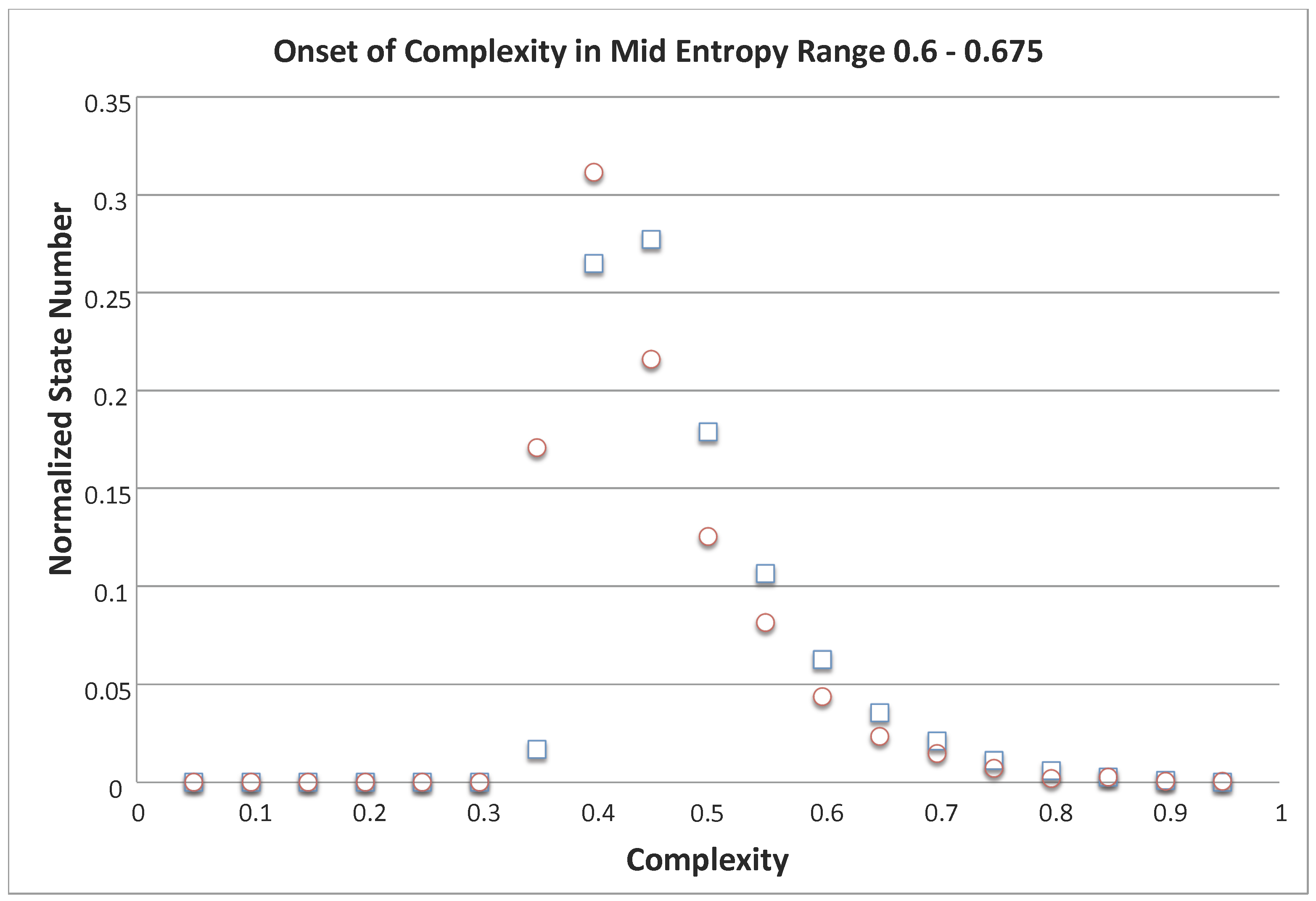
Figure 3 and Figure 4 add information regarding the density states that lie in the tree in each entropy/complexity area. First, we observe that the number of states near the middle of the two figures is far greater than in outer regions, as indicated by the brightly colored regions. Figure 5 shows a 2D plot of the density of states as a function of entropy. More interesting, however, is the distribution or density of states with similar incomparability in the normalized entropy region $0.6<\overline{S}<0.675$ shown in Figure 6. That figure is obtained by sorting the normalized incomparability numbers for the states in that entropy range and counting the number of states with similar incomparability numbers. (Incomparability increments were taken to be 0.05, and the normalization factor is the total number of states with entropy in the range between 0.6 and 0.675). Since all states in this entropy region have significant incomparability, Figure 6 is flat at first. Then, there is sudden increase in the density of states with similar incomparability, leading quickly to a maximum that then decays slowly. Thus, not only is complexity maximized near middle entropy, the density of states there is also highest. The implication of this observation is the subject of our ongoing investigations of dynamics (or evolution) on the YDL.

Currently, we are exploring an application of the mixing concept to DNA or RNA. DNA and RNA are long sequences of four basic nucleotides. It is known that three nucleotides form what is known as a codon, so there are only 64 possible codons that can be formed using only four nucleotides. It is also known that genes are collections of codons lying between two special codons called stop codons (of which there are only 3). Thus, a gene is understood to be a mixed set of N codons. To apply mixing to this problem we note that each gene has a mixing character determined by the distribution of codons in the gene. For example, let $n_1,n_2,n_3,\dots ,n_{61}$ be the number of codons of each type of codon in the gene (there are only 61 non-stop codons), then the mixing character of the gene is the partition of N, namely $[n_1,n_2,\dots ,n_{61}]$. Thus, for a genome consisting of thousands of genes, it is possible (after suitable normalization) [16] to employ majorization to determine the relative mixing of each of its genes.

5. Conclusions: Why This Is Different

The results shown in Figure 2, Figure 3, Figure 4, Figure 5 and Figure 6 are entirely quantitative and visualize the results of our analysis of the mixing partial order with regard to incomparability among Boltzmann states. The general convex shape of the incomparability vs. entropy curves shown in Figure 2 and Figure 3 has been suggested by many authors as characteristic of complexity [17]. However, their arguments leading to the shape are fundamentally different from ours. A complete review of all views of complexity is beyond the scope of this paper, so we will focus on what we feel is unique in this work.

Measuring complexity has a long history. In 2001, Lloyd listed 31 measures of complexity [18], and no doubt many more have been added in the past 15 years. Among his measures, the ones relating to the degree of organization are most relevant to the work here. Beginning in 1948 with Weaver [19], two types of complexity were identified: organized and disorganized. Disorganized complexity is associated with randomness while organized complexity is argued to occur as the result of interactions among members of the system. Johnson, however, recently adopted a definition for complexity science as “the study of the phenomena which emerge from a collection of interacting objects” [20]. This view of complexity has been adopted by many in the scientific community. Another important view of complexity has emerged from the study of the period doubling approach to deterministic chaos, [21,22,23,24,25,26]. In this approach, high complexity is argued to occur just prior to the onset of chaos. This view is quite different from the one here.

In contrast to both the chaos view and Johnson’s view of complexity, here we argue that complexity emerges when systems are characterized by members that are fundamentally incomparable rather than being due to interactions between them or to deterministic chaos. It is important to note that out view is based on quantitative results for a fundamental set of objects central to thermodynamic; namely Boltzmann states.

Because of the ubiquity of the Boltzmann distribution, it is likely that these results will also be of use in any system that relies on (1). See for example a clever adaptation of information theory by Rao and colleagues [27,28] to interpret a $4,000$ year old undeciphered Indus script. Another example is the use of Shannon information to characterize the correlations of chromosome sequences [29]. The fundamental insight provided by our research is that complexity emerges as a complement to entropy whenever there are states (objects, species, people, etc.) that are incomparable under a partial order.

The present work is independent of dynamics. In past work [15], we investigated the dynamics on the Hasse diagram for mixing of Boltzmann states showing the many evolutionary paths that can be taken from completely ordered states to completely disordered states. It is near the middle of the paths where we now find the most complexity in terms of incomparability. In future work, we will apply the incomparability idea to evolutions of other systems including ecosystems, economic systems, and organizational structures, where one often observes the rise and fall of complexity through time.