A Novel Operational Matrix of Caputo Fractional Derivatives of Fibonacci Polynomials: Spectral Solutions of Fractional Differential Equations

Abstract

Herein, two numerical algorithms for solving some linear and nonlinear fractional-order differential equations are presented and analyzed. For this purpose, a novel operational matrix of fractional-order derivatives of Fibonacci polynomials was constructed and employed along with the application of the tau and collocation spectral methods. The convergence and error analysis of the suggested Fibonacci expansion were carefully investigated. Some numerical examples with comparisons are presented to ensure the efficiency, applicability and high accuracy of the proposed algorithms. Two accurate semi-analytic polynomial solutions for linear and nonlinear fractional differential equations are the result.

1. Introduction

Fractional calculus is a vital branch of mathematical analysis which deals with derivatives and integrals to an arbitrary order (real or complex). There are intensive studies of fractional calculus from both theoretical and practical points of view. The applications of fractional calculus in many fields such as physics, economics, probability theory and statistics are numerous. For example, many physical and engineering models are described by fractional differential equations. For some applications of fractional calculus, one can refer to [1].

Due to the great importance of fractional differential equations (FDEs) and their applications in various disciplines, many researchers have shown considerable interest in developing numerical algorithms for solving these types of equations. Numerical solutions for various types of FDEs by applying several techniques were proposed, for instance, Adomian’s decomposition method [2,3], the Taylor collocation method [4], the variational iteration method [5], the finite difference method [6,7] and the ultraspherical wavelets method [8,9]. In addition, orthogonal polynomials have been widely used for obtaining numerical solutions for different types of FDEs. For example, Chebyshev polynomials of the second kind were employed by Sweilam et al. for solving space fractional-order diffusion equations [10]. Moreover, Chebyshev polynomials of the first kind were used for solving some fractional differential equations in Khader and Sweilam [11].

The three well-known versions of spectral methods; namely collocation, tau and Galerkin methods play pivotal roles in the numerical solutions of various types of differential equations. The spectral solutions are expressed in terms of truncated series of various polynomials. Actually, this solution is written as ∑a_kφ_k, where {φ_k} is a set of polynomials, which is often orthogonal. The expansion coefficients a_k can be determined by applying an appropriate spectral method. The collocation approach is performed by enforcing the differential equation to be satisfied exactly at some selected points called nodes or collocation points. The tau method is a synonym for expanding the residual function as a series of orthogonal polynomials and then, applying the boundary conditions as constraints. The Galerkin method is basically based on selecting some combinations satisfying the underlying boundary (initial) conditions as basis functions, and then, enforcing the residual to be orthogonal with the basis functions. This approach is fruitfully applied in many studies to solve two point linear boundary value problems (BVPs), in one and two dimensions [12,13,14,15].

The utilization of operational matrices of derivatives of different orthogonal polynomials is very effective for treating almost all types of differential equations. To be more precise, several operational matrices are employed for obtaining numerical solutions of ordinary differential equations. In this regard, Abd-Elhameed in [16] has developed a novel harmonic numbers operational matrix of derivatives to solve linear and nonlinear sixth-order BVPs. Likewise, Abd-Elhameed [17] and Doha et al. [18] used tau and Galerkin operational matrices of derivatives, respectively, to solve the singular Lane-Emden differential equations. The approach of employing the operational matrices is not limited to application in ordinary differential equations, but it can be also followed to handle FDEs. In this respect, a number of articles were devoted to introducing numerical solutions for these equations. In this respect, a Legendre operational matrix of fractional derivatives were constructed and employed for solving some types of FDEs in [19]. As well, Rostamy et al. [20] handled these equations with the aid of a Bernstein operational matrix of fractional derivatives. Other articles were interested in using the operational matrices of fractional integration to solve FDEs, i.e., Kazem [21].

The Fibonacci polynomials with their generalizations, and Fibonacci numbers and the golden ratio, are key elements in number theory. They have enormous applications in various disciplines such as computer science, statistics, physics, biology and graph theory [22]. Several studies were peformed to theoretically discuss Fibonacci polynomials and generalized Fibonacci polynomials (see [23,24,25]). However, as far we know, articles interested in using these polynomials in different applications are scarce. For example, a collocation procedure for treating BVPs based on using the Fibonacci operational matrix of derivatives has been developed in [26,27].

The principal objective of the present article is to present and implement new numerical spectral solutions of some types of FDEs. For this purpose, the operational matrix of fractional derivatives of Fibonacci polynomials are constructed, and then employed along with the tau and collocation spectral methods for obtaining numerical solutions of FDEs.

The paper is organized as follows: first, in Section 2, some preliminaries including some fundamental definitions of the fractional calculus theory are presented. This section also includes an overview on Fibonacci polynomials and their relevant properties. Section 3 is interested in constructing Fibonacci operational matrix of the fractional derivatives in the Caputo sense. Section 4 is devoted to implementing and presenting two numerical algorithms for solving two-term FDEs. Section 5 is interested in investigating the convergence and error analysis of the suggested expansion of Fibonacci polynomials. Some numerical examples and discussions are presented in Section 6, hoping to illustrate the efficiency, simplicity and applicability of the two proposed algorithms. Finally, some conclusions are reported in Section 7.

2. Preliminaries

2.1. Some Definitions and Properties of Fractional Calculus

In this subsection, some notations, definitions and preliminary facts about fractional calculus theory are presented.

Definition 1.

The Riemann–Liouville fractional integral operator $I^{\mu }$ of order μ on the usual Lebesgue space L₁ [0,1] is defined as:

$$I^{\mu }f(t)=\{\begin{array}{ll}\frac{1}{\Gamma (\mu )}{\int }_0^t{(t-\tau )}^{\mu -1}f(\tau )d\tau ,& \mu >0,\\ f(t),& \mu =0.\end{array}$$

where the following properties are satisfied:

(i)

I^μI^v = I^{μ +v}

(ii)

I^μI^v = I^vI^μ

(iii)

$I^{\mu }{t}^v=\frac{\Gamma \left(\mathrm{v}+1\right)}{\Gamma \left(\mathrm{v}+\mathsf{\mu }+1\right)}{t}^{\mu +v}$

where μ > −1 and v > −1.

Definition 2.

The Riemann–Liouville fractional derivative of order μ > 0 is defined by:

$$\begin{array}{ccc}(D_{*}^{\mu }f)(t)={\left(\frac{d}{dt}\right)}^n(I^{n-\mu }f)(t),& n-1<\mu <n,& n\in {\rm N}.\end{array}$$

Definition 3.

The fractional differential operator in Caputo sense is defined as:

$$\begin{array}{ccc}(D^{\mu }f)(t)=\frac{1}{\Gamma (n-\mu )}{\int }_0^t{(t-\tau )}^{n-\mu -1}{f}^{(n)}(\tau )d\tau ,& \mu >0,& t>0,\end{array}$$

where, n − 1 < μ < n, n ∈ N.

The operator D^μ satisfies the following basic properties for n − 1 < μ < n:

$$(D^{\mu }{I}^{\mu }f)(t)=f(t),$$

$$\begin{array}{cc}(I^{\mu }{D}^{\mu }f)(t)=f(t)-{\displaystyle \sum _{k=0}^{n-1}}\frac{f^{(k)}(0^{+})}{k!}{t}^k,& t>0,\end{array}$$

$$\begin{array}{ccc}{D}^{\mu }{t}^k=\frac{\Gamma (k+1)}{\Gamma (k+1-\mu )}{t}^{k-\mu },& k\in \mathbb{N},& k\ge \lceil \mu \rceil ,\end{array}$$

(1)

where the ceiling notation ⌈μ⌉ denotes the smallest integer greater than or equal to μ. For more properties of fractional derivatives and integrals, see for example [28,29].

2.2. Some Properties of Fibonacci Polynomials

It is well-known that the Fibonacci polynomials may be constructed by the following recurrence relation

$$F_{m+2}(x)=x{F}_{m+1}(x)+F_m(x),m\ge 0,$$

with the initial values:

$$\begin{array}{cc}{F}_0(x)=0,& F_1(x)=1.\end{array}$$

These polynomials have the following explicit form:

$$F_m(x)=\frac{{\left(x+\sqrt{x^2+4}\right)}^m-{\left(x-\sqrt{x^2+4}\right)}^m}{2^m\sqrt{x^2+4}}.$$

Moreover, they can be represented by the following power form:

$$F_m(x)={\displaystyle \sum _{r=0}^{\lfloor \frac{m-1}{2}\rfloor }}\left(\begin{array}{c}m-r-1\\ r\end{array}\right)x^{m-2r-1},$$

(2)

where the notation ⌊z⌋ represents the largest integer less than or equal to z .

The first derivative of Fibonacci polynomials is related with the original Fibonacci polynomials by the following relation (see [30]):

$$\begin{array}{cc}\frac{d{F}_{m+1}(x)}{dx}={\displaystyle \sum _{i=0}^{\lfloor \frac{m-1}{2}\rfloor }}{(-1)}^i(m-2i)F_{m-2i}(x),& m\ge 1.\end{array}$$

Furthermore, the polynomials x^m can be written as a combination of Fibonacci polynomials as (see [30]):

$$x^m={\displaystyle \sum _{i=0}^{\lfloor \frac{m}{2}\rfloor }}{(-1)}^i\left[\left(\begin{array}{c}m\\ i\end{array}\right)-\left(\begin{array}{c}m\\ i-1\end{array}\right)\right]F_{m-2i+1}(x),m\ge 0.$$

(3)

It is usefull to rewrite relations (2) and (3) as:

$$F_i(x)={\displaystyle \sum _{\begin{array}{c}j=0\\ (j+i)odd\end{array}}^i}\frac{\left(\frac{i+j-1}{2}\right)!}{j!\left(\frac{i-j-1}{2}\right)!}{x}^j,i\ge 0,$$

(4)

$$x^m=m!{\displaystyle \sum _{\begin{array}{c}j=1\\ (j+m)odd\end{array}}^{m+1}}\frac{{(-1)}^{\frac{m-j+1}{2}}j}{\left(\frac{m-j+1}{2}\right)!\left(\frac{m+j+1}{2}\right)!}{F}_j(x),m\ge 0.$$

(5)

respectively.

3. Construction of the Fibonacci Operational Matrix of the Caputo Fractional Derivative

Assume that u(x) is a square Lebesgue integrable function on (0,1). In addition, assume that u(x) can be expanded as:

$$u(x)={\displaystyle \sum _{k=1}^{\infty }}{c}_k{F}_k(x).$$

If we kept only the first (n + 1) terms of Fibonacci polynomials, then:

$$u(x)\approx u_n(x)={\displaystyle \sum _{k=1}^{n+1}}{c}_k{F}_k(x)=C^T\Phi (x),$$

where

$$C^T=[c_1,c_2,\dots ,c_{n+1}],$$

and

$$\Phi (x)={[F_1(x),F_2(x),\dots ,F_{n+1}(x)]}^T.$$

(6)

Now, the first derivative of the vector Φ(x) can be written as:

$$\frac{d\Phi (x)}{dx}=M^{(1)}\Phi (x),$$

(7)

where $M^{\left(1\right)}=\left(m_{ij}^{\left(1\right)}\right)$ is the Fibonacci operational matrix of derivatives of order (n + 1) × (n + 1). Moreover, the elements of $M^{\left(1\right)}$ are given explicitly as:

$$m_{ij}^{(1)}=\{\begin{array}{cc}{(-1)}^{\frac{i-j+3}{2}}(j+1),& i>j,(i+j)odd,\\ 0,& otherwise.\end{array}$$

For example, for n = 6, the operational matrix $M^{\left(1\right)}$ is:

$$M^{(1)}={\left(\begin{array}{ccccccc}0& 0& 0& 0& 0& 0& 0\\ 1& 0& 0& 0& 0& 0& 0\\ 0& 2& 0& 0& 0& 0& 0\\ -1& 0& 3& 0& 0& 0& 0\\ 0& -2& 0& 4& 0& 0& 0\\ 1& 0& -3& 0& 5& 0& 0\\ 0& 2& 0& -4& 0& 6& 0\end{array}\right)}_{7\times 7}.$$

Introducing a Fibonacci Operational Matrix of Fractional Derivatives

The principal goal of this section is to introduce a generalization of the operational matrix of the integer case. First note that relation (7) leads to the relation:

$$\frac{d^s\Phi (x)}{d{x}^s}=M^{(s)}\Phi (x)={\left(M^{(1)}\right)}^s\Phi (x),$$

where s is any postive integer. The following theorem gives the Fibonacci operational matrix of fractional derivatives:

Theorem 1.

If Φ(x) is the Fibonacci polynomial vectors which defined in Equation (6), then for any α > 0, the following relation holds:

$$D^{\alpha }\Phi (x)=x^{-\alpha }{M}^{(\alpha )}\Phi (x),$$

where $M^{\left(\alpha \right)}=\left\{m_{ij}^{\alpha }\right)$ is the (n + 1) × (n + 1) Fibonacci operational matrix of derivatives of order α in Caputo sense and it is given explicitly as:

$$M^{\left(\alpha \right)}=\left(\begin{array}{ccccc}0& 0& 0& \cdots & 0\\ ⋮& ⋮& ⋮& & ⋮\\ {\xi }_{\alpha }(\lceil \alpha \rceil ,1)& {\xi }_{\alpha }(\lceil \alpha \rceil ,\lceil \alpha \rceil )& 0& \cdots & 0\\ ⋮& ⋮& ⋮& & ⋮\\ {\xi }_{\alpha }(i,1)& \cdots & {\xi }_{\alpha }(i,i)& \cdots & 0\\ ⋮& ⋮& ⋮& & ⋮\\ {\xi }_{\alpha }(n+1,1)& {\xi }_{\alpha }(n+1,2)& {\xi }_{\alpha }(n+1,3)& \cdots & {\xi }_{\alpha }(n+1,n+1)\end{array}\right).$$

In fact, the elements $\left(m_{ij}^{\alpha }\right)$ are given explicitly by:

$$m_{i,j}^{\alpha }=\{\begin{array}{ll}{\xi }_{\alpha }(i,j),& i\ge \lceil \alpha \rceil ,i\ge j;\\ 0,& otherwise.\end{array}$$

where

$${\xi }_{\alpha }(i,j)=j{\displaystyle \sum _{\begin{array}{c}k=\lceil \alpha \rceil \\ (i+k)odd\\ (j+k)odd\end{array}}^i}\frac{{(-1)}^{\frac{k-j+1}{2}}k!\left(\frac{i+k-1}{2}\right)!}{\left(\frac{i-k-1}{2}\right)!\left(\frac{k-j+1}{2}\right)!\left(\frac{k+j+1}{2}\right)!\Gamma (k+1-\alpha )}.$$

(8)

Proof. 

If we apply D^α to Equation (4), then with the aid of relation (1), the following relation is obtained:

$$D^{\alpha }{F}_i(x)={\displaystyle \sum _{\begin{array}{c}k=\lceil \alpha \rceil \\ (k+i)odd\end{array}}^i}\frac{\left(\frac{i+k-1}{2}\right)!}{\left(\frac{i-k-1}{2}\right)!\Gamma (k+1-\alpha )}{x}^{k-\alpha }.$$

The inversion formula (5) enables one—after performing some manipulations—to write:

$$D^{\alpha }{F}_i(x)=x^{-\alpha }{\displaystyle \sum _{j=1}^i}{\xi }_{\alpha }(i,j)F_j(x),$$

(9)

where ξ_α(i,j) is given in (8).

Now Equation (9) can be rewritten in the following vector form:

$$\begin{array}{cc}{D}^{\alpha }{F}_i(x)=x^{-\alpha }[{\xi }_{\alpha }(i,1),{\xi }_{\alpha }(i,2),\dots ,{\xi }_{\alpha }(i,i),0,0,\dots ,0]\Phi (x),& \lceil \alpha \rceil \le i\le n+1,\end{array}$$

(10)

and also we can write:

$$\begin{array}{cc}{D}^{\alpha }{F}_i(x)=x^{-\alpha }[0,0,\dots ,0],& 1\le i\le \lceil \alpha \rceil -1.\end{array}$$

(11)

Finally, Equation (10) together with Equation (11) yield the desired result. □

4. Two New Matrix Algorithms for Solving Fractional-Order Differential Equations

This section is devoted to analyzing and presenting two numerical algorithms for solving fractional-order linear and nonlinear differential equations based on using the constructed Fibonacci operational matrix. The two algorithms, namely, the tau Fibonacci matrix method (TFMM) and the collocation Fibonacci matrix method (CFMM) are employed for solving linear and nonlinear multi-term orders fractional differential equations, respectively.

4.1. Use of TFMM for Handling Linear Fractional Differential Equations

Consider the linear fractional differential equation ([31,32]):

$$\begin{array}{ccc}{D}^{\alpha }u(x)+p(x)D^{\beta }u(x)+q(x)u(x)=f(x),x\in (0,1),& \alpha \in (q_1,1+q_1],\beta \in (q_2,1+q_2],& q_1\ge q_2,\end{array}$$

(12)

subject to the initial conditions:

$$\begin{array}{cc}{u}^{(i)}(0)=a_i,& i=0,1,\dots ,q_1,\end{array}$$

(13)

or the boundary conditions:

$$\{\begin{array}{l}\begin{array}{ccccc}{u}^{(i)}(0)=a_i,& u^{(i)}(1)=b_i,& i=0,1,\dots ,\frac{q_1-1}{2},& if& q_{1}odd,\end{array}\\ \begin{array}{cccccc}{u}^{(i)}(0)=a_i,& u^{(i)}(1)=b_i,& u^{(\frac{q_1}{2})}(0)=a,& i=0,1,\dots ,\frac{q_1}{2}-1,& if& q_{1}even.\end{array}\end{array}$$

(14)

Now, assume that u(x) can be approximated as:

$$u(x)\approx u_n(x)=C^T\Phi (x).$$

(15)

In virtue of Theorem 1, D^αu(x) and D^βu(x) can be approximated as:

$$D^{\alpha }u(x)\approx x^{-\alpha }{C}^T{M}^{(\alpha )}\Phi (x),$$

(16)

and

$$D^{\beta }u(x)\approx x^{-\beta }{C}^T{M}^{(\beta )}\Phi (x).$$

(17)

Making use of the approximations in (15)–(17), the residual of (12) can be calculated by the formula:

$$x^{\alpha }R(x)=C^T{M}^{(\alpha )}\Phi (x)+p(x)x^{\alpha -\beta }{C}^T{M}^{(\beta )}\Phi (x)+q(x)x^{\alpha }{C}^T\Phi (x)-x^{\alpha }f(x),$$

and accordingly the application of tau method (see [18]) yields:

$$\begin{array}{cc}{\int }_0^1{x}^{\alpha }R(x)F_i(x)dx=0,& i=1,2,\dots ,n-q_1.\end{array}$$

(18)

Moreover, the initial conditions (13) yield:

$$\begin{array}{cc}{C}^T{M}^{(i)}\Phi (0)=a_i,& i=0,1,\dots ,q_1,\end{array}$$

(19)

while the boundary conditions (14) yield:

$$\{\begin{array}{l}\begin{array}{llllll}{C}^T{M}^{(i)}\Phi (0)=a_i,& C^T{M}^{(i)}\Phi (1)=b_i,& i=0,1,\dots ,\frac{q_1-1}{2},& if& q_1& odd\end{array}\\ \begin{array}{lllllll}{C}^T{M}^{(i)}\Phi (0)=a_i,& C^T{M}^{(i)}\Phi (1)=b_i,& C^T{M}^{(\frac{q_1}{2})}\Phi (0)=a,& i=0,1,\dots ,\frac{q_1}{2}-1,& if& q_1& even.\end{array}\end{array}$$

(20)

From Equation (18) with (19) or (20), a linear system of equations in the unknown expansion coefficients c_i of dimension (n + 1) can be generated. Thanks to the Gaussian elimination technique or any suitable technique, this system can be solved, and consequently, the approximate solution (15) can be found.

4.2. Use of CFMM for Handling Nonlinear Fractional Differential Equations

Consider the following nonlinear fractional-order differential equation:

$$\begin{array}{ccc}{D}^{\alpha }u(x)=\Omega \left(D^{\beta }u(x),u(x),x\right),x\in (0,1),& \alpha \in (q_1,1+q_1],\beta \in (q_2,1+q_2],& q_1\ge q_2,\end{array}$$

(21)

subject to the initial conditions (13) or the boundary conditions (14).

We approximate u(x), D^αu(x) and D^βu(x) as in the previous section, hence the residual $\tilde{R}\left(x\right)$ of Equation (21) is given by:

$$\tilde{R}(x)=x^{-\alpha }{C}^T{M}^{(\alpha )}\Phi (x)-\Omega \left(x^{-\beta }{C}^T{M}^{(\beta )}\Phi (x),C^T\Phi (x),x\right).$$

The application of the spectral collocation method requires that $\tilde{R}\left(x\right)$ must vanish at certain collocation points. We select the collocation points to be: $\frac{i}{n+1},i=1,2,\dots ,n-q_1,$ and therefore:

$$\begin{array}{cc}\tilde{R}\left(\frac{i}{n+1}\right)=0,& i=1,2,\dots ,n-q_1.\end{array}$$

(22)

Equations (22) with (19) or (20) generate a nonlinear system of equations in the unknown expansion coefficients c_i of dimension (n + 1). Newton’s iterative technique can be employed for solving this system, and consequently, the approximate solution is obtained from (15).

Remark 1.

It is worthy to mention here that the CFMM, which described above, can be also applied to linear fractional differential equations.

5. Convergence and Error Analysis

In this section, a comprehensive study of the convergence and error analysis of the suggested expansion of Fibonacci polynomials is performed. For this purpose, the following Lemmas are needed.

Lemma 1 (Byrd [33]).

If f(x) is an infinitely differentiable function at the origin, then f(x) can be expanded in terms of Fibonacci polynomials as:

$$f(x)={\displaystyle \sum _{k=1}^{\infty }}{\displaystyle \sum _{j=0}^{\infty }}\frac{k{(-1)}^j{a}_{2j+k-1}}{2^{2j+k-1}(j+k)}\left(\begin{array}{c}2j+k-1\\ j\end{array}\right)F_k(x),$$

where

$$a_i=\frac{f^{(i)}(0)}{i!}.$$

Lemma 2 (Abramowitz et al. [34]).

Let I_v(x) denote the modified Bessel function of order v of the first kind. The following identity holds:

$${\displaystyle \sum _{j=0}^{\infty }}\frac{x^j}{2^{j}j!(j+k)!}={\left(\frac{2}{x}\right)}^{\frac{k}{2}}{I}_k(\sqrt{2x}).$$

Lemma 3 (Luke [35]).

The modified Bessel function of the first kind I_v(x) satisfies the following inequality:

$$\begin{array}{cc}\left|I_{\nu }(x)\right|\le \frac{x^{\nu } \text{cosh} x}{2^{\nu }\Gamma (\nu +1)},& \forall x>0.\end{array}$$

Lemma 4.

If $\sigma =\frac{1+\sqrt{5}}{2}$ denotes the golden ratio, then the following inequality is valid:

$$\begin{array}{cc}{F}_k(x)\le {\sigma }^{k-1}& \forall x\in [0,1].\end{array}$$

Proof. 

We have:

$$F_k(x)\le F_k(1)=\frac{1}{\sqrt{5}}\left({\left(\frac{1+\sqrt{5}}{2}\right)}^k-{\left(\frac{1-\sqrt{5}}{2}\right)}^k\right)\le {\sigma }^{k-1}.$$

□

The following two theorems discuss the convergence and error analysis of the Fibonacci expansion.

Theorem 2.

If f(x) is defined on [0, 1] with $\left|f^{\left(i\right)}\left(0\right)\right|\le M^i, i\ge 0,M$ is a positive constant and $f\left(x\right)={\sum }_{k=1}^{\infty }{c}_k{F}_k\left(x\right)$, then we have:

• $\left|c_k\right|\le \frac{M^{k-1}\text{cosh}M}{2^{k-1}\left(k-1\right)!}$.
• The series converges absolutely. 

Proof. 

Starting from Lemma 1, we have:

$$\left|c_k\right|=k\left|{\displaystyle \sum _{j=0}^{\infty }}\frac{{(-1)}^j{f}^{(2j+k-1)}(0)}{2^{2j+k-1}j!(j+k)!}\right|\le k{\displaystyle \sum _{j=0}^{\infty }}\frac{M^{2j+k-1}}{2^{2j+k-1}j!(j+k)!},$$

and therefore the application of Lemma 2 implies that:

$$\left|c_k\right|\le \frac{2k}{M}{I}_k(M).$$

(23)

The inequality in (23) along with Lemma 3 leads to the inequality in the first part.

Now, to prove that the series ${\sum }_{k=1}^{\infty }{c}_k{F}_k\left(x\right)$ converges absolutely, the comparison test is applied. Making use of the first part along with Lemma 4, yields $\left|c_k{F}_k\left(x\right)\right|\le \frac{\text{cosh}M}{\left(k-1\right)!}{\left(\frac{M\sigma }{2}\right)}^{k-1}$ but ${\sum }_{k=1}^{\infty }\frac{\text{cosh}M}{\left(k-1\right)!}{\left(\frac{M\sigma }{2}\right)}^{k-1}=coshM{e}^{M\sigma /2}$ and therefore the series converges absolutely. □

Theorem 3.

If f(x) satisfies the hypothesis of Theorem 2, and $e_n\left(x\right)={\sum }_{k=n+2}^{\infty }{c}_k{F}_k\left(x\right)$ then we have the following error estimate:

$$\left|e_n(x)\right|<\frac{\text{cosh} M{\left(M \sigma \right)}^{n+1}{e}^{\frac{M \sigma }{2}}}{2^{n+1}(n+1)!}.$$

Proof. 

By Theorem 2, we can write:

$$\left|e_n(x)\right|\le \text{cosh} M{\displaystyle \sum _{k=n+2}^{\infty }}\frac{{\mu }^{k-1}}{(k-1)!}, \mu =\frac{M \sigma }{2},$$

which can be written as:

$$\left|e_n(x)\right|\le e^{\mu }\text{cosh} M\left(1-\frac{\Gamma (n+1,\mu )}{\Gamma (n+1)}\right),$$

where Γ(n + 1) and Γ(n + 1,μ) denote the well-known gamma function and the incomplete gamma function, respectively (see [36]).

Now, we have $\left|e_n\left(x\right)\right|\le \frac{e^{\mu }\text{cosh}M}{\Gamma \left(n-1\right)}{\int }_0^{\mu }{t}^n{e}^{-t}dt$ but since $e^{-t}\langle 1, \forall t\rangle 0.$ Therefore we have $\left|e_n\left(x\right)\right|\le \frac{e^{\mu }\text{cosh}M{\mu }^{n+1}}{\left(n-1\right)!}$ which completes the proof of the theorem. □

6. Numerical Tests

This section presents some numerical experiments and comparisons to illustrate the efficiency and applicability of the two proposed algorithms in this paper.

Example 1 (Doha et al. [37]).

Consider the following linear fractional initial value problem

$$\begin{array}{cc}{D}^{2}u(x)+D^{\frac{1}{2}}u(x)+u(x)=x^2+\frac{8}{3\sqrt{\pi }}{x}^{\frac{3}{2}}+2,& x\in (0,1),\end{array}$$

(24)

$$u(0)=u^{\prime }(0)=0.$$

(25)

We apply TFMM for the case n = 2. The residual of Equation (24) can be calculated by the formula:

$$\sqrt{x}R(x)=\sqrt{x}{C}^T{M}^{(2)}\Phi (x)+C^T{M}^{(\frac{1}{2})}\Phi (x)+\sqrt{x}{C}^T\Phi (x)-\left(x^{\frac{5}{2}}+\frac{8}{3\sqrt{\pi }}{x}^2+2\sqrt{x}\right)$$

where the operational matrices M⁽²⁾ and M^(½) are given explicitly as follows:

$$\begin{array}{cc}{M}^{(2)}=\left(\begin{array}{ccc}0& 0& 0\\ 0& 0& 0\\ 2& 0& 0\end{array}\right),& M^{(\frac{1}{2})}=\frac{1}{\sqrt{\pi }}\left(\begin{array}{lll}0& 0& 0\\ 0& 2& 0\\ -\frac{8}{3}& 0& \frac{8}{3}\end{array}\right).\end{array}$$

If we apply the method which described in Section 4.1 to Equation (24), then we get:

$$(32+100\sqrt{\pi })c_3+(40+15\sqrt{\pi })c_2+30\sqrt{\pi }{c}_1=32+70\sqrt{\pi }.$$

(26)

Moreover, the initial conditions (25) yield:

$$c_3+c_1=0, \text{and} c_2=0.$$

(27)

Equations (26) and (27) can be immediately solved to give c₁ = −1, c₂ =0, c₃ = 1, and consequently u(x) = x² which is the exact solution.

Example 2 (Doha et al. [38]).

Consider the following inhomogeneous Bagley–Trovik equation:

$$\begin{array}{cc}{D}^{2}u(x)+D^{\frac{3}{2}}u(x)+u(x)=f(x),& x\in (0,1),\\ u(0)=0,& u^{\prime }(0)=\alpha ,\end{array}$$

(28)

where f(x) is chosen such that the exact solution of Equation (28) is u(x) = sin(αx). We apply the two methods, namely, TFMM, CFMM for different values of α and n. In

Table 1. Comparison between TFMM and CSM in [38] for Example 2.

n	α = 1			α = 4π
	TFMM	CFMM	CSM [38]	TFMM	CFMM	CSM [38]
4	1.0 × 10−4	3.4 × 10−5	3.4 × 10−4	7.2 × 10−3	8.2 × 10−4	3.9 × 100
8	9.1 × 10−7	2.7 × 10−8	4.3 × 10−7	5.8 × 10−6	1.5 × 10−6	4.7 × 10−1
16	5.3 × 10−12	4.9 × 10−13	1.8 × 10−8	5.7 × 10−11	7.4 × 10−13	3.5 × 10−5
32	6.2 × 10−14	9.8 × 10−16	7.1 × 10−10	2.6 × 10−13	2.2 × 10−14	1.4 × 10−6

, we display a comparison between the results obtained if the two methods TFMM, CFMM are applied with the results obtained by applying Chebyshev spectral method (CSM) which developed in [38]. The displayed results in this table show that our algorithm gives a lesser error in almost all cases.

Example 3 ([32,39]).

Consider the following linear boundary value problem:

$$\begin{array}{c}\begin{array}{cccc}{D}^{q_1}u(x)-D^{q_2}u(x)=-1-e^{x-1},& x\in (0,1),& q_1\in (1,2],& q_2\in (0,1],\end{array}\\ u(0)=u(1)=0\end{array}$$

(29)

The exact solution of (29) in the case corresponds to q₁ = 2 and q₂ = 1 is u(x) = x(1 − e^x–1). In

Table 2. Comparison between TFMM and [32,39] for Example 3.

x	[39]	[32]	TFMM	Exact
0.1	0.05934820	0.05934383	0.05934303	0.05934303
0.2	0.05934820	0.11013431	0.11013421	0.11013421
0.3	0.11014318	0.15102443	0.15102441	0.15102441
0.4	0.15103441	0.18047562	0.18047535	0.18047535
0.5	0.19673826	0.19673476	0.19673467	0.19673467
0.6	0.19780653	0.19780804	0.19780797	0.19780797
0.7	0.18142196	0.18142748	0.18142725	0.18142725
0.8	0.14500893	0.14501561	0.14501540	0.14501540
0.9	0.08564186	0.08564683	0.08564632	0.08564632

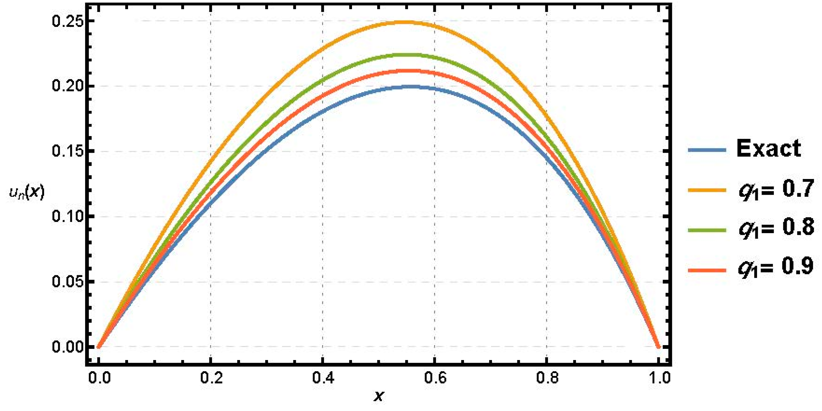
, we compare our results with those obtained in [32,39]. Figure 1 illustrates that the approximate solutions in the case corresponds to q₂ = 2 and for various values of q₁ near the value 1, have similar behavior.

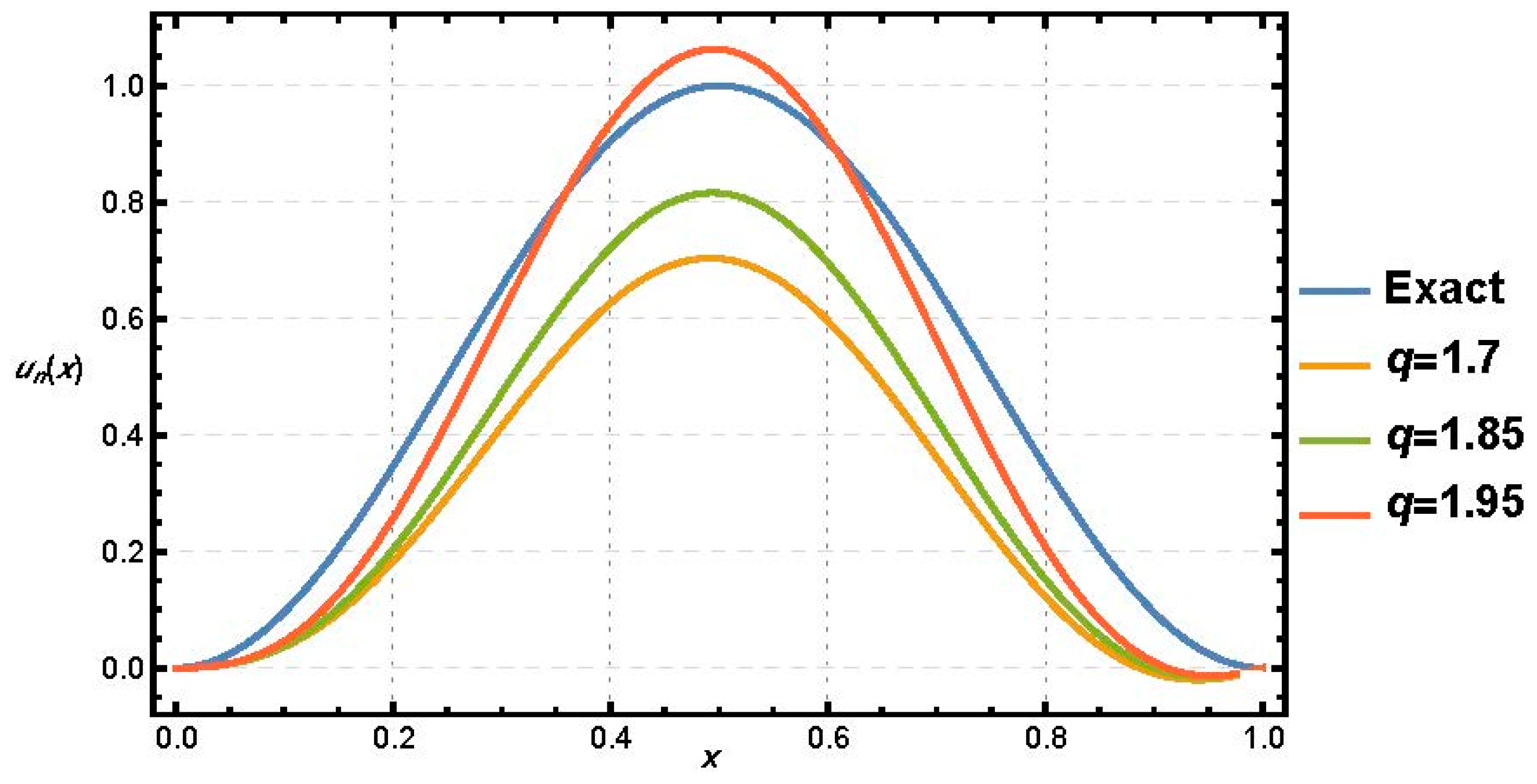
Example 4 ([32,39]).

Consider the following nonlinear boundary value problem:

$$\begin{array}{ccc}{D}^{q}u(x)-u^2(x)=2{\pi }^2\text{cos}(2\pi x)-{\text{sin}}^4(\pi x),& x\in (0,1),& q\in (1,2),\end{array}$$

(30)

subject to the homogenous boundary conditions:

$$u(0)=u(1)=0.$$

The exact solution of Equation (30) for the case q = 2 is u(x) = sin²(πx) We apply CFMM.

Table 3. Maximum absolute error of Example 4.

n	3	5	7	9	11	13	15
Error	5.2 × 10−3	2.0 × 10−6	3.4 × 10−8	5.9 × 10−10	4.7 × 10−12	1.6 × 10−14	1.2 × 10−16

lists the maximum pointwise error of Equation (30) for the case q = 2 and different values of n. Figure 2 illustrates that the behavior of the approximate solution for values of q near 2 is somehow close to the behavior of the exact solution.

Example 5 ([40]).

Consider the fractional Van der Pol equation with fractional damping:

$$\begin{array}{ccc}{D}^{\alpha +\beta }u(x)+\eta (u^2(x)-1)D^{\alpha }u(x)+u(x)=a\text{sin}(\omega x),& x\in (0,1),& \alpha +\beta \le 2,\end{array}$$

(31)

subject to the homogenous initial conditions:

$$u(0)=u^{\prime }(0)=0.$$

We solve Equation (31) for the case corresponds to a = 1.31, ω = 0.5. In

Table 4. Comparison between CFMM and [40] for Example 5 in case α = β = 1, η = 0.1.

x	[40] n = 6	[40] n = 15	Runge–Kutta	CFMM n = 6	CFMM n = 10
0.1	0.000149	0.000119	0.000109	0.000108	0.000109
0.2	0.001000	0.000894	0.000876	0.000878	0.000876
0.3	0.003113	0.002980	0.002953	0.002958	0.002953
0.4	0.007227	0.007022	0.006987	0.006983	0.006987
0.5	0.013976	0.013647	0.013603	0.013607	0.013603
0.6	0.023709	0.023454	0.023403	0.023405	0.023403
0.7	0.037322	0.037010	0.036952	0.036952	0.036952
0.8	0.055164	0.054838	0.054775	0.054774	0.054775
0.9	0.077783	0.077416	0.077348	0.077347	0.077348

, we compare our results with the numerical solution obtained in [40] and the solution obtained from Mathematica 9 by applying the fourth-order Runge–Kutta method. In

Table 5. Comparison between TFMM and [40] for Example 5.

x	0.1	0.3	0.5	0.7	0.9
[40] n = 120	2.36 × 10−7	8.15 × 10−7	1.54 × 10−6	2.42 × 10−6	3.42 × 10−6
TFMM n = 12	2.57 × 10−10	3.22 × 10−10	5.27 × 10−10	9.58 × 10−10	7.81 × 10−10

, we compare our results with the results obtained in [40] in case with no damping η = 0.

Remark 2.

The results of Table 5 indicate that the numerical spectral solutions obtained by CFMM are in high agreement with the solutions of the fourth order Runge-Kutta method, also it is more accurate than the results obtained in Maleknejad [40] with the same number of retained modes.

Example 6 ([40]).

Consider the fractional Rayleigh equation with fractional damping:

$$\begin{array}{ccc}{u}^{″}(x)+\gamma (1-\frac{1}{3}{(D^{\alpha }u(x))}^2)u^{\prime }(x)+u(x)=0,& x\in (0,1),& 0<\alpha <2,\end{array}$$

(32)

subject to the initial conditions:

$$u(0)=1, u^{\prime }(0)=0.$$

We solve Equation (32) for the case corresponds to γ = 0.1, 0.5. In

Table 6. Comparison between CFMM n = 10 and [40] n = 15 for Example 6.

x	γ = 0.1			γ = 0.5
	[40]	Runge–Kutta	CFMM	[40]	Runge–Kutta	CFMM
0.1	0.994977	0.995021	0.995021	0.995047	0.995086	0.995086
0.2	0.980157	0.980198	0.980198	0.980681	0.980712	0.980712
0.3	0.955739	0.955775	0.955775	0.957446	0.957468	0.957468
0.4	0.922054	0.922085	0.922085	0.925977	0.925992	0.925992
0.5	0.879519	0.879543	0.879543	0.886946	0.886953	0.886953
0.6	0.828629	0.828646	0.828646	0.841048	0.841046	0.841046
0.7	0.769953	0.769962	0.769962	0.788998	0.788988	0.788988
0.8	0.704126	0.704126	0.704126	0.731528	0.731510	0.731510
0.9	0.631845	0.631835	0.631835	0.669382	0.669356	0.669356

we give a comparison between CFMM and the operational matrix method developed in Maleknejad [40] for the case corresponds to α = 1, γ = 0.1, 0.5.

Remark 3.

From the numerical results of Table 6, we conclude that CFMM with fewer number of terms is compared favorably with the fourth-order Runge-Kutta solution obtained from Mathematica.

Example 7. 

Consider the following fractional differential equation:

$$\begin{array}{cc}{u}^{(9.5)}(x)=e^{x}erf(\sqrt{x}),& x\in (0,1),\end{array}$$

(33)

subject to the initial conditions:

$$\begin{array}{cc}{u}^{(r)}(0)=1,& 0\le r\le 9,\end{array}$$

where, $erf\left(x\right)=\frac{2}{\sqrt{\pi }}{\int }_0^x{e}^{-t^2}dt$.

The exact solution of Equation (33) is u(x) = e^x. To illustrate the advantages of our method if compared with methods which employ orthogonal polynomials, We solve Equation (33) by our proposed algorithm namely, TFMM, and also by using Legendre spectral tau method (LSTM).

Table 7. Comparison between LSTM and TFMM for solving Example 7.

n		14	16	18	20	22	24
LSTM	E	2.3 × 10−4	3.7 × 10−6	6.5 × 10−8	3.8 × 10−10	6.2 × 10−12	9.1 × 10−15
	t	37.407	45.781	61.573	70.594	86.247	107.241
TFMM	E	6.5 × 10−5	8.1 × 10−8	9.7 × 10−10	6.2 × 10−12	2.9 × 10−14	3.7 × 10−16
	t	28.891	36.212	39.847	48.827	63.952	74.528

presents a comparison between the maximum pointwise errors which resulted from the application of TFMM and LSTM for different values of n. In addition, a comparison between the running times (in seconds) if the two methods are applied is also displayed in Table 7. The results of this table indicate the advantages of our method if compared with LSTM. Moreover, they ensure that TFMM is efficient for higher order fractional differential equations.

Remark 4:

From the obtained numerical results in Table 1, Table 2, Table 3, Table 4, Table 5, Table 6 and Table 7 and the obtained estimates in Theorems 2 and 3, we list here the advantages of the current work:

(1) 

The generation of Fibonacci Polynomials is very easy either from the recurrence relation or from the direct definition. 

(2) 

The implementation of Fibonacci polynomials is efficient compared to the orthogonal polynomials in other words. The running time of the “Mathematica” code is very short compared with using the orthogonal polynomials. 

(3) 

The speed of convergence of Fibonacci polynomials (inverse factorial rate of convergence) is very efficient. Theorem 2 ensures this result. 

7. Conclusions

In this work, two numerical algorithms for solving linear and nonlinear two-term fractional order differential equations are developed. The basic idea behind the proposed algorithms is based on constructing a new operational matrix of fractional derivatives of Fibonacci polynomials to reduce both linear and nonlinear fractional differential equations to systems of linear or nonlinear algebraic equations which can be solved efficiently. As far as we know, the derived Fibonacci operational matrix of fractional derivatives is novel and it is the first time to use such matrix in solving fractional-order differential equations. The tested numerical examples show the high efficiency and performance of the proposed algorithms.

References

1. Hilfer, R. Applications of Fractional Calculus in Physics; World Scientific Publishing: Singapore, 2000. [Google Scholar]
2. Daftardar-Gejji, V.; Jafari, H. Solving a multi-order fractional differential equation using Adomian decomposition. Appl. Math. Comput. 2007, 189, 541–548. [Google Scholar] [CrossRef]
3. Momani, S.; Odibat, Z. Numerical approach to differential equations of fractional order. J. Comput. Appl. Math. 2007, 207, 96–110. [Google Scholar] [CrossRef]
4. Çenesiz, Y.; Keskin, Y.; Kurnaz, A. The solution of the Bagley–Torvik equation with the generalized Taylor collocation method. J. Frankl. Inst. 2010, 347, 452–466. [Google Scholar] [CrossRef]
5. Das, S. Analytical solution of a fractional diffusion equation by variational iteration method. Comput. Math. Appl. 2009, 57, 483–487. [Google Scholar] [CrossRef]
6. Meerschaert, M.M.; Tadjeran, C. Finite difference approximations for two-sided space-fractional partial differential equations. Appl. Numer. Math. 2006, 56, 80–90. [Google Scholar] [CrossRef]
7. Sweilam, N.H.; Khader, M.M.; Nagy, A.M. Numerical solution of two-sided space-fractional wave equation using finite difference method. J. Comput. Appl. Math. 2011, 235, 2832–2841. [Google Scholar] [CrossRef]
8. Abd-Elhameed, W.M.; Youssri, Y.H. New spectral solutions of multi-term fractional-order initial value problems with error analysis. Comput. Model. Eng. Sci. 2015, 105, 375–398. [Google Scholar]
9. Abd-Elhameed, W.M.; Youssri, Y.H. New ultraspherical wavelets spectral solutions for fractional Riccati differential equations. Abstr. Appl. Anal. 2014, 2014, 626275. [Google Scholar] [CrossRef]
10. Sweilam, N.H.; Nagy, A.M.; El-Sayed, A.A. Second kind shifted Chebyshev polynomials for solving space fractional order diffusion equation. Chaos Soliton Fractals 2015, 73, 141–147. [Google Scholar] [CrossRef]
11. Khader, M.M.; Sweilam, N.H. On the approximate solutions for system of fractional integro-differential equations using Chebyshev pseudo-spectral method. Appl. Math. Model. 2013, 37, 9819–9828. [Google Scholar] [CrossRef]
12. Doha, E.H.; Abd-Elhameed, W.M.; Bassuony, M.A. New algorithms for solving high even-order differential equations using third and fourth Chebyshev–Galerkin methods. J. Comput. Phys. 2013, 236, 563–579. [Google Scholar] [CrossRef]
13. Doha, E.H.; Abd-Elhameed, W.M.; Bassuony, M.A. On the coefficients of differentiated expansions and derivatives of Chebyshev polynomials of the third and fourth kinds. Acta Math. Sci. 2015, 35, 326–338. [Google Scholar] [CrossRef]
14. Doha, E.H.; Abd-Elhameed, W.M. Efficient solutions of multidimensional sixth-order boundary value problems using symmetric generalized Jacobi-Galerkin method. Abstr. Appl. Anal. 2012, 2012, 749370. [Google Scholar] [CrossRef]
15. Abd-Elhameed, W.M.; Doha, E.H.; Youssri, Y.H. Efficient spectral-Petrov-Galerkin methods for third-and fifth-order differential equations using general parameters generalized Jacobi polynomials. Quaest. Math. 2013, 36, 15–38. [Google Scholar] [CrossRef]
16. Abd-Elhameed, W.M. On solving linear and nonlinear sixth-order two point boundary value problems via an elegant harmonic numbers operational matrix of derivatives. Comput. Model. Eng. Sci. 2014, 101, 159–185. [Google Scholar]
17. Abd-Elhameed, W.M. New Galerkin operational matrix of derivatives for solving Lane–Emden singular type equations. Eur. Phys. J. Plus 2015, 130. [Google Scholar] [CrossRef]
18. Doha, E.H.; Abd-Elhameed, W.M.; Youssri, Y.H. Second kind Chebyshev operational matrix algorithm for solving differential equations of Lane–Emden type. New Astron. 2013, 23–24, 113–117. [Google Scholar] [CrossRef]
19. Saadatmandi, A.; Dehghan, M. A new operational matrix for solving fractional-order differential equations. Comput. Math. Appl. 2010, 59, 1326–1336. [Google Scholar] [CrossRef]
20. Rostamy, D.; Alipour, M.; Jafari, H.; Baleanu, D. Solving multi-term orders fractional differential equations by operational matrices of BPs with convergence analysis. Rom. Rep. Phys. 2013, 65, 334–349. [Google Scholar]
21. Kazem, S. An integral operational matrix based on Jacobi polynomials for solving fractional-order differential equations. Appl. Math. Model. 2013, 37, 1126–1136. [Google Scholar] [CrossRef]
22. Koshy, T. Fibonacci and Lucas Numbers with Applications; Wiley: Hoboken, NJ, USA, 2011. [Google Scholar]
23. Wang, W.; Wang, H. Some results on convolved (p,q)-Fibonacci polynomials. Integral Transforms Spec. Funct. 2015, 26, 340–356. [Google Scholar] [CrossRef]
24. Zhang, W. On Chebyshev polynomials and Fibonacci numbers. Fibonacci Q. 2002, 40, 424–428. [Google Scholar]
25. Gulec, H.H.; Taskara, N.; Uslu, K. A new approach to generalized Fibonacci and Lucas numbers with binomial coefficients. Appl. Math. Comput. 2013, 220, 482–486. [Google Scholar] [CrossRef]
26. Koc, A.B.; Cakmak, M.; Kurnaz, A.; Uslu, K. A new Fibonacci type collocation procedure for boundary value problems. Adv. Differ. Equ. 2013, 2013, 262. [Google Scholar] [CrossRef]
27. Mirzaee, F.; Hoseini, S.F. Application of Fibonacci collocation method for solving Volterra–Fredholm integral equations. Appl. Math. Comput. 2016, 273, 637–644. [Google Scholar] [CrossRef]
28. Oldham, K.B.; Spanier, J. The Fractional Calculus: Theory and Applications of Differentiation and Integration to Arbitrary Order; Dover Publications: Mineola, NY, USA, 1974. [Google Scholar]
29. Podlubny, I. Fractional Differential Equations: An Introduction to Fractional Derivatives, Fractional Differential Equations, to Methods of Their Solution and Some of Their Applications; Academic Press: Cambridge, MA, USA, 1998. [Google Scholar]
30. Falcon, S.; Plaza, A. On k-Fibonacci sequences and polynomials and their derivatives. Chaos Soliton Fractals 2009, 39, 1005–1019. [Google Scholar] [CrossRef]
31. Rehman, M.; Khan, R.A. The Legendre wavelet method for solving fractional differential equations. Commun. Nonlinear Sci. Numer. Simul. 2011, 16, 4163–4173. [Google Scholar] [CrossRef]
32. Keshavarz, E.; Ordokhani, Y.; Razzaghi, M. Bernoulli wavelet operational matrix of fractional-order integration and its applications in solving the fractional-order differential equations. Appl. Math. Model. 2014, 38, 6038–6051. [Google Scholar] [CrossRef]
33. Byrd, P.F. Expansion of analytic functions in polynomials associated with Fibonacci numbers. Fibonacci Q. 1963, 1, 16–27. [Google Scholar]
34. Abramowitz, M.; Stegun, I.A. Handbook of Mathematical Functions: With Formulas, Graphs, and Mathematical Tables; Dover Publications: Mineola, NY, USA, 1964; p. 1046. [Google Scholar]
35. Luke, Y.L. Inequalities for generalized hypergeometric functions. J. Approx. Theory 1972, 5, 41–65. [Google Scholar] [CrossRef]
36. Rainville, E.D. Special Functions; Macmillan: London, UK, 1960; p. 365. [Google Scholar]
37. Doha, E.H.; Bhrawy, A.H.; Ezz-Eldien, S.S. A Chebyshev spectral method based on operational matrix for initial and boundary value problems of fractional order. Comput. Math. Appl. 2011, 62, 2364–2373. [Google Scholar] [CrossRef]
38. Doha, E.H.; Bhrawy, A.H.; Ezz-Eldien, S.S. Efficient Chebyshev spectral methods for solving multi-term fractional orders differential equations. Appl. Math. Model. 2011, 35, 5662–5672. [Google Scholar] [CrossRef]
39. Wang, Y.G.; Song, H.F.; Li, D. Solving two-point boundary value problems using combined homotopy perturbation method and Green’s function method. Appl. Math. Comput. 2009, 212, 366–376. [Google Scholar] [CrossRef]
40. Maleknejad, K.; Torkzadeh, L. Application of hybrid functions for solving oscillator equations. Rom. J. Phys. 2015, 60, 87–98. [Google Scholar]
Figure 1. Different solutions of Example 3: x vs. un(x).
Entropy 18 00345 g001
Figure 2. Different solutions of Example 4: x vs. un(x).
Entropy 18 00345 g002