Article

Towards the Development of a Universal Expression for the Configurational Entropy of Mixing

Nuclear Material Department, GIA, GAATN, Bariloche Atomic Center, 8400 Bariloche, Río Negro, Argentina
Entropy 2016, 18(1), 5; https://doi.org/10.3390/e18010005
Submission received: 28 May 2015 / Revised: 12 August 2015 / Accepted: 2 September 2015 / Published: 31 December 2015

Abstract

:
This work discusses the development of analytical expressions for the configurational entropy of different states of matter using a method based on the identification of the energy-independent complexes (clustering of atoms) in the system and the calculation of their corresponding probabilities. The example of short-range order (SRO) in Nb-H interstitial solid solution is used to illustrate the choice of the atomic complexes and their structural changes with H concentration, providing an alternative methodology to describe critical properties. The calculated critical composition of the miscibility gap is xc = 0.307, in remarkable agreement with the experimental value of xc ~ 0.31. The same methodology is applied to deduce the equation of state (EOS) of a hard sphere system. The EOS is suitable to describe the percolation thresholds and fulfills both the low and random close packing limits. The model, based on the partition of the space into Voronoi cells, can be applied to any off-lattice system, thus introducing the possibility of computing the configurational entropy of gases, liquids and glasses with the same level of accuracy.

1. Introduction

The development of analytical expressions for the configurational entropy of mixing was an active field of research several decades ago. Empirical or theoretical expressions and methods were deduced in each field of condensed matter. Several examples can be found in the literature, such as: (i) the expressions of Flory [1] and Huggins [2] for linear polymer solutions; (ii) the cluster variation method (CVM) [3] and cluster site approximation (CSA) [4] for the study of order-disorder and phase equilibrium in alloys; and (iii) the Gibbs and Di Marzio expression [5] for glasses, to cite just some of the best known expressions in each field. Each model has its own area of application and research. For example, CVM cannot be applied to polymer solutions, and Flory’s expression is not suitable for the study of order-disorder in alloys. However, the traditional methodology, based on the calculation of the number of configurations, had restrictions in the development of expressions in complex systems, such as interstitial solid solutions or liquids and amorphous materials. Although an enormous amount of work has been carried out in both fields of research, the deduction of accurate analytical expressions for the configurational entropy of mixing has been very elusive due to the complicated underlying physics. While the difficulties with interstitial solutions are due to the blocking effects, the difficulties with gases, liquids, amorphous materials and glasses are derived from the almost insurmountable task of computing the number of configurations in a system without lattice periodicity. The limitations arise because all previous models compute the number of configurations using the lattice gas model under the following assumptions: (i) athermal mixture or non-interacting atoms, atomic complexes, molecules or associated chemical species, which leave their internal properties unaffected; (ii) no superposition among chemical species; (iii) the equivalence of all N lattice sites; and (iv) the use of a rigid lattice with no distortion and constant volume.
The field of research related to interstitial solid solutions is an illustrative example of the difficulties encountered in computing the configurational entropy of mixing if the assumption of no superposition between chemical species is abandoned. Although there are several analytical expressions that can be used to compute the entropy of mixing in these systems, they are all approximated or limited to low or medium solute concentrations. In addition, they all assume a random distribution of interstitial atoms in the interstitial sub-lattice, and consequently, the interaction between defects is not considered in previous models, i.e., no short-range order (SRO) description is possible. Furthermore, they cannot describe the differences between chemical and elastic blocking and their influence on the configurational entropy. It is important to note that there is experimental and theoretical evidence to show that the random blocking model (RBM) [6] assumed in this kind of solid solution is not appropriate in a number of systems, such as hcp R-H (R = Sc, Y, Lu) [7,8,9], bcc Nb-H [10] and Zr-H systems [11].
A similar situation to that of interstitial solutions, as regards the encoding of structural information into a compact expression, is found in gases, liquids, amorphous materials and glasses. In these systems, the lack of periodicity of the atomic arrangements makes deduction of a universal and unique structural description a very difficult task, leaving many questions unanswered. Consequently, the deduction of an analytical and parameter-free expression for the configurational entropy of mixing of multicomponent systems, valid for any non-crystalline states of matter, remains a largely unsolved problem.
The development of such a model, involving counting the number of configurations, is an impractical idea. However, a recent formalism to compute configurational entropy, based on the identification of energetically independent complexes within the mixture and the calculation of their respective probabilities, offers an opportunity to consider this proposal seriously. The importance of such an idea is not only academic in nature, i.e., the development of a unified description for all states of matter, it originates from the need to develop general expressions with the same level of accuracy for each state of matter so as to obtain a precise description of their physical properties and phase diagrams. This work shows that it is possible to develop such a model, but major theoretical and computational effort will be required. In order to achieve this goal, a set of atomic complexes (clustering of atoms), which can describe, simultaneously, the basic structural features of liquids, glasses and solids, must be found. The first step towards such a formulation is discussed in this work, based on several inspiring previous works related to a hard sphere system [12,13,14], metallic glasses [15,16,17,18], the CVM method [3] and a recently deduced analytical expression for interstitial solutions [10,11].
As the first step in this research on off-lattice systems, the configurational entropy for the hard sphere system is computed based on the Voronoi partition of space. The deduced equation of state (EOS) fulfills both the low and random close packing limits and describes the percolation thresholds. In addition, the methodology is suitable for application to any system with no lattice periodicity, such as liquids, glasses and amorphous materials.

2. Probabilistic Description of the Configurational Entropy of Mixing

2.1. The Model

The entropy of a classical system with a discrete set of microstates is given by the Gibbs’ expression: S = −kBPilnPi, where kB is Boltzmann’s constant. The index i labels all of the microstates with energy Ei (i = 1,…,W), and Pi is the probability of finding a particular configuration of the ensemble consistent with a given energy value. If all microstates are equivalent with the same probability Pi = P = 1/W, Boltzmann’s expression for the configurational entropy is deduced: S = −kBln(P) = kBln(W). Thus, the configurational entropy has usually been calculated by computing the number of configurations W. Nevertheless, it was shown that this property can also be deduced by computing probabilities through the inverse problem: S = −kBln(P) [19]. The probability P is a conditional one, and its analytical determination is usually very difficult. However, if the assumption of energy independent complexes in the mixture is used, the conditional probability can be written as a product of independent probabilities. Therefore, if the complexes in the mixture can be identified, the configurational entropy is written as,
S = k B ln ( P ) = k B ln ( i p i n i ) = k B i n i ln p i
where ni and pi are the numbers and probabilities of each independent complex i in the mixture, respectively. Thus, Equation (1) could constitute a complement to the traditional method of computing the configurational entropy, helping in the identification and understanding of the representative physical features in complicated systems, such as interstitial solutions or amorphous materials.
One point worthy of comment here is related to the nature of the complexes existing in the mixture: What are these complexes? How should they be selected? The methodology presented in this work shows that a thorough understanding of the physical properties of the system is necessary in order to correctly identify the complexes and their changes with composition, temperature and, eventually, lattice distortion. The following sections will explain how to select the complexes and deduce analytical expressions for interstitial solutions, which can describe SRO and a parameter-free EOS for a hard sphere system.

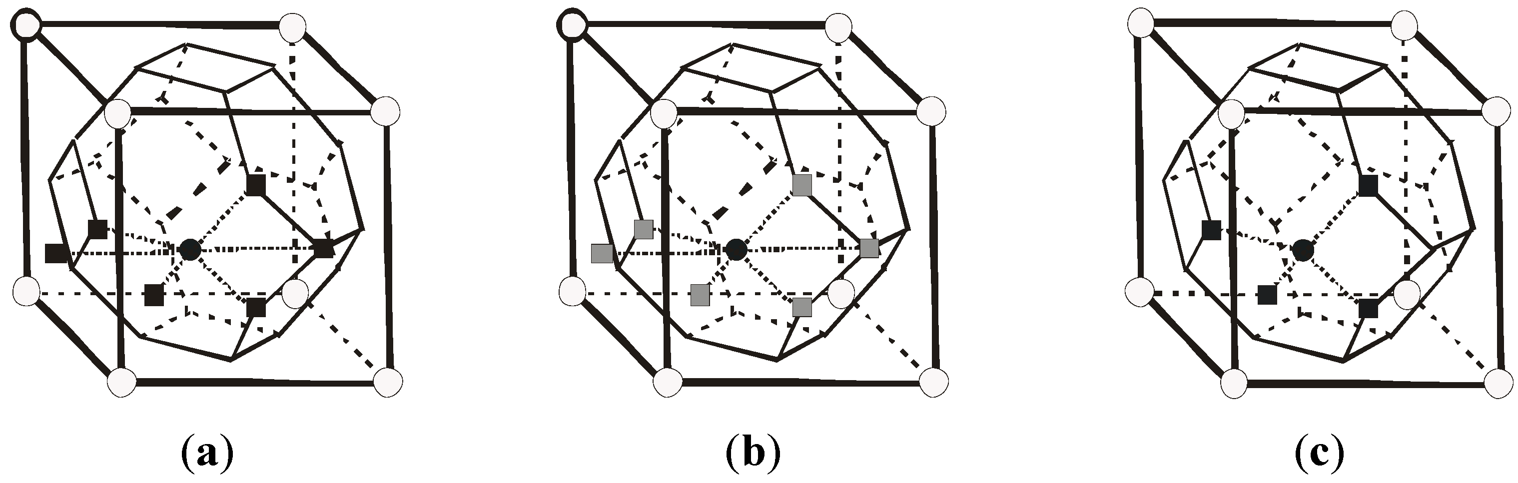
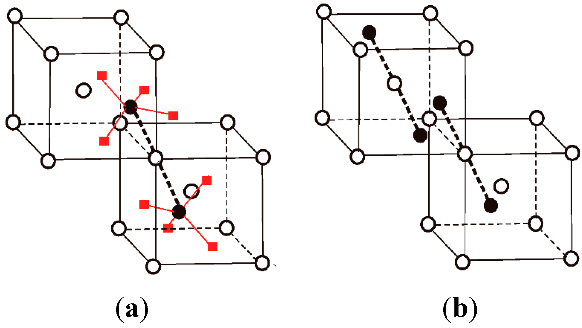
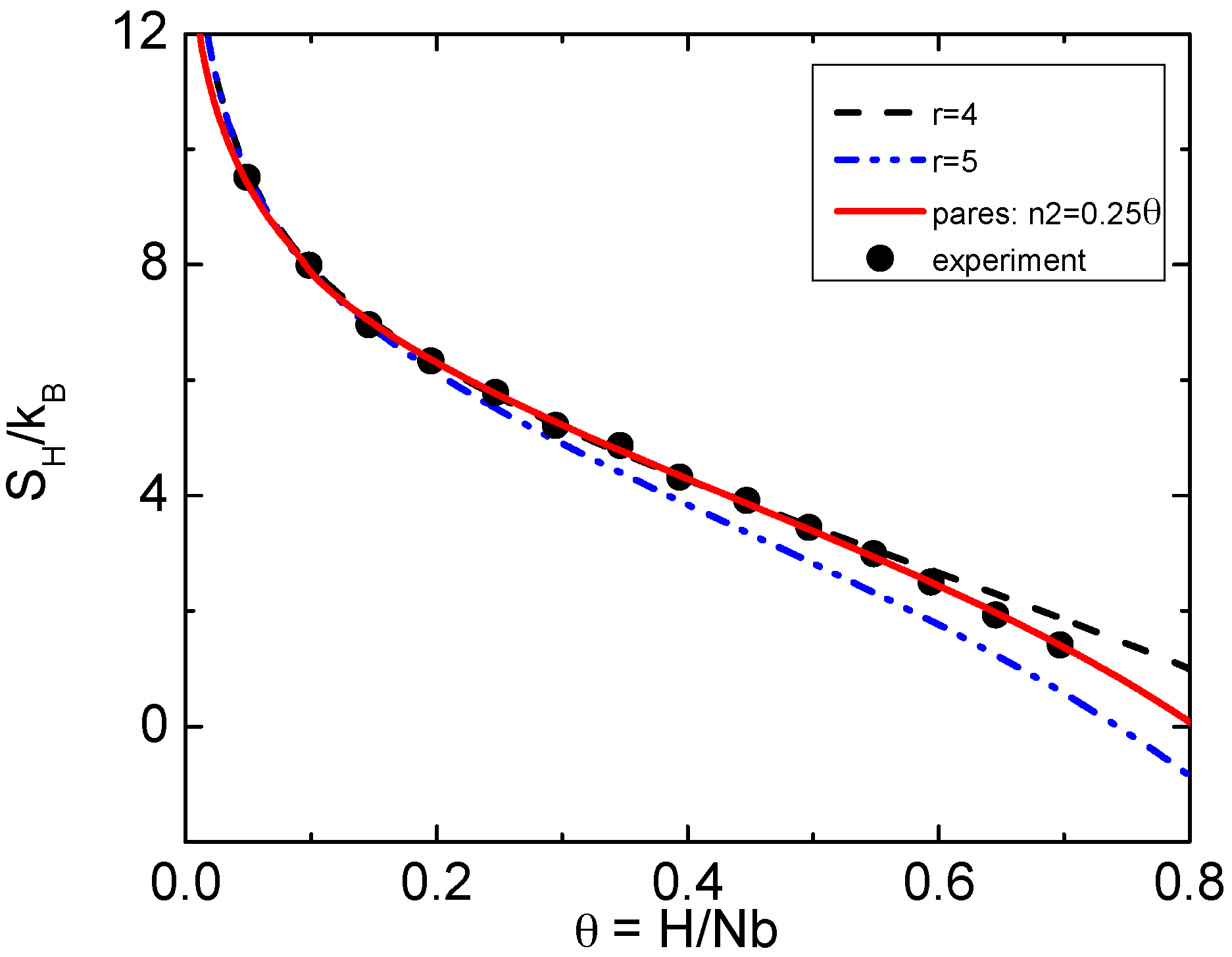
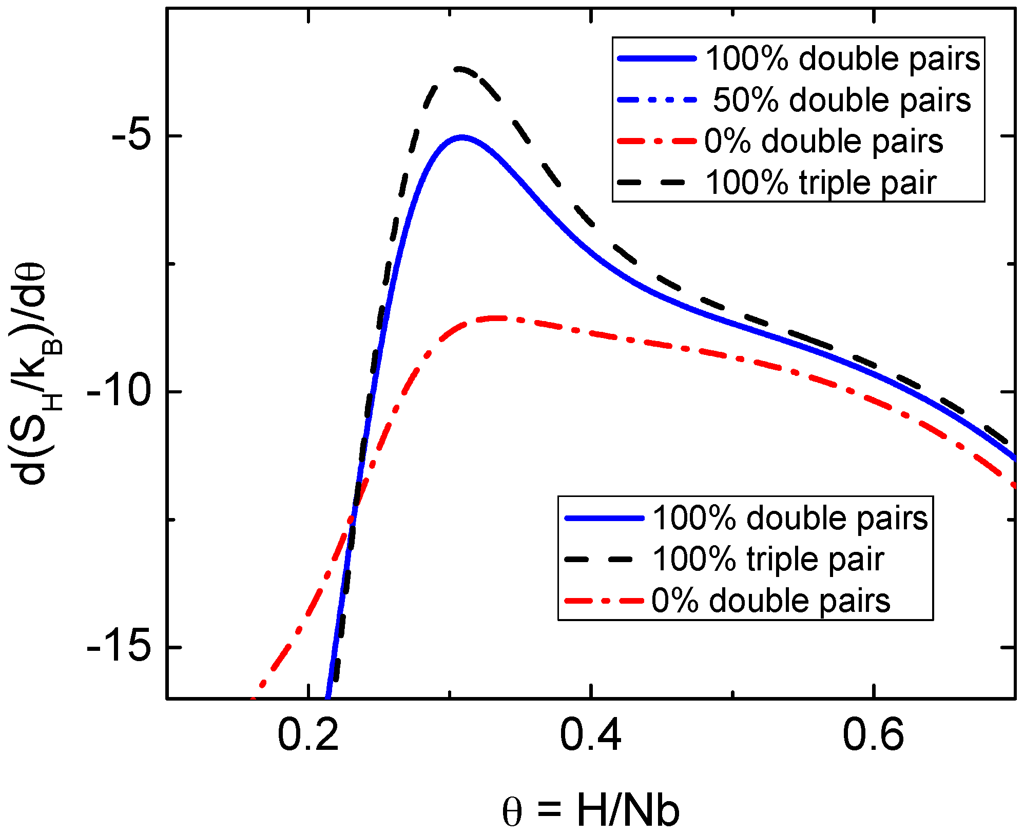
2.2. Selection of the Complexes and the Critical Composition of the Miscibility Gap in the Nb-H Interstitial Solid Solution

It has been mentioned previously that the source of the difficulties in modeling interstitial solutions arises from the site blocking effects, where the occupation of an interstitial site is prevented by the prior occupation of a neighboring interstitial site. There is an effective repulsion, which may be chemical and/or strain in origin. The number of blocked vacancies inhibited for occupancy by other interstitials and, consequently, the size r of the blocking sphere depend on the magnitude of this repulsive interaction.
The first step in modeling any interstitial solid solution is the choice of the number of blocked vacancies associated with each interstitial atom. The resulting structure with size r0 will be called the “basic complex” in this work. In the case of the Nb-H system, this selection is mainly related to the length of the H-H interaction. Several models have been developed in the literature according to the information selected to deduce this length. Figure 1 shows a comparison between the different models for the configurational entropy of mixing available in the literature for Nb-H based on the random blocking model (RBM) [19,20,21,22,23,24,25] and the experimental data from Veleckis and Edwards [26]. The RBM assumes a random mixture of H atoms. Although the configurational entropy data are well described by the models of [19,22,25], shown in Figure 2a,b, they all give a solubility limit around H/Nb = 1.5, in disagreement with the experimental value of H/Nb = 1.21 ± 0.04 measured at 750 K [25]. This limit can be described within the model of Figure 2c, a hard or total blocking of first neighbors, but it is incompatible with the experimental data, as shown in Figure 1 for the model of [19] with a blocking sphere of size r = 5.
Thus, there are two models for the blocking sphere, represented in Figure 2a,b, which correctly describe the configurational entropy data, but not the solubility limit, and one model, shown in Figure 2c, doing the opposite. What is the solution to the controversy between the solubility limit and the size of the basic complex? At this point, more experimental information should be used. The critical composition of the miscibility gap located at a concentration of H/Nb = θc = 0.31 in the phase diagram could be helpful in finding an explanation for this inconsistency.
In order to compute the maximum of the miscibility gap through the condition (∂2∆G/∂x2)xc = 0 [27,28], it is necessary to know the enthalpy of formation ΔH and the free energy G of the solid solution. The calculations of the thermodynamic properties in the cluster field approximation by Vaks and Orlov [29] suggest considerable temperature dependence, but an almost linear behavior of the ΔH vs. θ in the composition range 0 < θ < 0.4. Consequently, the extreme condition in this range is due only to an extreme in the configurational entropy, since the non-configurational partial molar entropy of mixing of the hydrogen is assumed, as usual, to be independent of temperature and composition [28]. Figure 3 shows the critical composition predicted by models plotted in Figure 1. All of these models give a critical composition around or above θ = 0.4, adding more confusion to the unexplained physical behavior of H in the Nb-H system.
Figure 1. The partial configurational entropy of the Nb-H system. Comparison between experimental data and theoretical models available in the literature. The theoretical results are adjusted to the lowest experimental values. The O’Keeffe model [25] displays similar behavior to Boureau’s model [22]. The data for the McLellan model is taken from [20].
Entropy 18 00005 g001
Figure 2. Basic complex or blocking sphere in the Nb-H system for: (a) hard blocking of first and second neighbors with size r0 = 7 [22]; (b) soft blocking of first and second neighbors with size r0 = 4 [19]; (c) hard blocking of first neighbors with size r0 = 5 [10]. Empty circles: Nb host lattice atoms. Full circle: H atom. Dark square: hard blocked vacancies. Grey square: soft blocked vacancies. (b and c are reproduced with permission from [10]).
Entropy 18 00005 g002
In order to find a model that correctly describes the H behavior, it is necessary to develop an adequate theoretical tool that should include SRO and the experimental evidence not taken into account by all previous models. A simple, general analytical expression overcoming the previous cited limitations has recently been deduced [10,11]. This expression, suitable for the treatment of interstitial clustering and SRO, is applicable to tetrahedral or octahedral interstitial solutions in any crystal lattice and for all interstitial concentrations.
Figure 3. Location of the critical composition of the miscibility gap from different models. Solid line: Speiser and Spretnak. Dotted line: Boureau [22] (see Figure 2a). Dashed line: Garcés [19] (see Figure 2b). Dot-dash line: O’Keeffe [25]. Short dash line: Ogawa [19]. None of these models describe the experimental critical composition value of θc = 0.31.
Entropy 18 00005 g003
The required theoretical tool is given by the following expression,
S N = k B [ i θ i ln ( θ i β j ( r j 1 ) θ j ) + ( β j r j θ j ) ln ( β j r j θ j β j ( r j 1 ) θ j ) ]
where the indices i and j label all of the interstitial complex and free vacancies in the mixture. β is the number of interstitial sites per metal atom, and θi = ni/N is the composition of each independent complex in the solid solution. See [10] for a detailed deduction of this expression.
The model given by Equation (2) provides the basis for an explanation of unsolved controversies in this system, such as: (1) inconsistencies between the solubility limit and the size of the basic complex, i.e., the size of the blocking sphere; (2) the inaccuracy of the different models regarding the configurational entropy of mixing; (3) the critical composition of the miscibility gap; (4) the length of the H-H interaction; (5) the nature of the α- and α’-phases; and (6) the structural relation between the disordered and ordered phases observed at low temperatures and compositions θ = H/Nb > 0.75. In addition, there are several experimental results that cannot be explained by the RBM, such as: (1) different experimental [30,31] and theoretical [32,33,34,35,36,37,38] results suggest that the H-H interaction is characterized by a repulsive interaction extending out to the third or fourth shell of the interstitial lattice and by an elastic interaction energy outside the radius of repulsion; however, these results contradict the assumptions of the RBM characterized by H-H repulsion up to second nearest neighbors; and (2) there is experimental evidence of SRO at very dilute H concentrations (<1 at% H) [39]) and in the α’-phase [40,41].
None of these experimental results can be explained using the RBM or even the CVM methods [38]. This fact shows that the underlying physics of the Nb-H system is still not properly identified, and the complexes selected by previous models are not representative of the H behavior. It is clear from a comparison between the models that the basic source of the controversies related to the Nb-H solid solution is the size of the basic complex and its change with H concentration.
How can the controversies previously cited be solved using Equation (2)? The first step is to find the size of the basic complex satisfying the solubility limit, given by β/r0. The experimental solubility limit of the solid solution, H/Nb = 1.21 ± 0.04 [25], can only be described in a bcc lattice (β = 6) if a basic complex of size r0 = 5 is assumed; see Figure 2c. This assumption is incompatible with the experimental data for the configurational entropy, as shown in Figure 1. However, a combination of basic complexes, arising from SRO, can also describe this limit. The simplest complex fulfilling the previous condition is a pair of H atoms with size r = 10, as shown in Figure 4a.
Figure 4. Composed objects formed in the solid solutions due to short-range order (SRO): (a) a pair H-Nb-H with the respective blocked vacancies and (b) a double pair (the blocked vacancies are not shown). Empty circles: Nb host lattice atoms. Full circle: H atom. Squares: blocked vacancies.
Entropy 18 00005 g004
The configurational entropy derived from Equation (2) for a mixture of vacancies, isolated H atoms and pairs is,
S k B N = θ 1 ln ( θ 1 6 4 θ 1 9 θ 2 ) + θ 2 ln ( θ 2 6 4 θ 1 9 θ 2 ) + ( 6 5 θ 1 10 θ 2 ) ln ( 6 5 θ 1 10 θ 2 6 4 θ 1 9 θ 2 )
In this expression, θ1 is the composition of isolated interstitial atoms and θ2 the H pair concentration, verifying the relation θI = θ1 + 2θ2. The growth of pairs has been computed by two phenomenological models:
(i)
a linear function: θ2 = A θI
(ii)
a sigmoid function, such as:
θ 2 = A 1 + e B ( θ C ) θ I
The parameters for the sigmoid function are: A = 0.10, B = 20 and C = 0.21. The sigmoid growth with A = 0.10 means that 18% of the H interstitial atoms are located in pairs. The partial configurational entropy is computed numerically and plotted in Figure 5. The result shows excellent agreement with the experimental data, giving a critical composition at θc = 0.33, as Figure 6 shows. The critical composition of the miscibility gap is not correctly described, and the phenomenology responsible for the gap is still elusive. Therefore, what is the H physical behavior in this system that makes it possible to explain accurately only the configurational entropy and the solubility limit?
Figure 5. The partial configurational entropy of the Nb-H system. Comparison between experimental data and theoretical models presented in this work. Solid line: a random mixture of vacancies (blocking sphere of size r0 = 1), isolated H atoms (blocking sphere of size r0 = 5) and pairs (blocking sphere of size r0 = 10). Dashed line: random mixture of vacancies and random H atoms (blocking sphere of size r0 = 4). Dash-dot line: random mixture of vacancies and random H atoms (blocking sphere of size r0 = 5).
Entropy 18 00005 g005
Figure 6. Location of the critical composition of the miscibility gap with the amount of pair clustering. An extreme is found at θc = 0.307 if all the pairs are assumed to form double or triple pairs, in remarkable agreement with the experimental value of θc = 0.31.
Entropy 18 00005 g006
A major problem in materials science is the description of the critical points. Sophisticated and powerful methods, such as CVM, fail in these areas due to the huge size of the basic cluster necessary to describe the long-range fluctuations near the critical point. However, what could the description of the current model be if we consider that in the vicinity of the critical point, the basic complex changes with H concentration? The result of θc = 0.33, very close to the experimental critical composition, indicates that the miscibility gap could be related to an additional structural process, e.g., the clustering or ordering of pairs beginning at a critical composition θc > 0. The present methodology can be applied easily to modeling of the pair clustering if all of the pairs in the mixture are assumed to form double or triple pairs. For this purpose, the same parameters obtained from fitting Equation (4) to the experimental data are used.
The configurational entropy expression for a mixture of vacancies of size r = 1, isolated H atoms with size r = 5 and double pairs with size r = 20 fulfilling the relation θI = θ1 +4 is,
S k B N = θ 1 ln ( θ 1 6 4 θ 1 19 θ 4 ) + θ 2 ln ( θ 4 6 4 θ 1 19 θ 4 ) + ( 6 5 θ 1 20 θ 4 ) ln ( 6 5 θ 1 20 θ 4 6 4 θ 1 19 θ 4 )
The same expression for triple pairs with size r = 30 fulfilling the relation θI = θ1 + 6θ6 is,
S k B N = θ 1 ln ( θ 1 6 4 θ 1 29 θ 6 ) + θ 2 ln ( θ 6 6 4 θ 1 29 θ 6 ) + ( 6 5 θ 1 20 θ 4 ) ln ( 6 5 θ 1 30 θ 6 6 4 θ 1 29 θ 6 )
Figure 6 shows the location of the partial configurational entropy maximum with the amount of double or triple pairs in the mixture. The model gives a critical composition for the miscibility gap of θc = 0.307, in remarkable agreement with the experimental value of θc = 0.31.
The possibility of including SRO and the change of the complexes with the H concentration in the entropy formalism allows an explanation for several controversies in Nb-H, giving a physical picture different from the usual model based on a random mixture of H atoms. The current model makes it possible to solve the contradictions between the length of the H-H interaction and the experimental solubility limit. Moreover, it proposes that the α-phase could be formed by a random mixture of H atoms and H-Nb-H pairs, and the α’-phase could be characterized mainly by double or triple pairs in addition to H interstitials. The location of the maximum of the miscibility gap is related to the formation of a double or triple pair in the solid solution. It is also proposed in the current model that the double or triple pair configuration could be interpreted as the seed for the ordered phases observed experimentally for H concentrations greater than θ = 0.75. The interested reader can find details of the relation between pairs and the ordered phases in [10].

3. Non-Crystalline States of Matter

The example of Nb-H interstitial solution showed that Equation (1) provides a useful framework for the deduction of an analytical expression for the configurational entropy of mixing if the atomic complexes, or local structures, vs. H concentration can be identified. The difficulties encountered to solve the same problem by counting the number of configurations have also been shown. Gases, liquids and metallic glasses are other very elusive systems for the traditional methodology due to their lack of periodicity. Is it possible to describe all of these states of matter using the same structural model and the framework provided by Equation (1)? Quantitative description of local structures is a requirement when studying amorphous systems, such as granular matter or metallic glasses. While granular structures are disordered, metallic glasses display various degrees of structural ordering beyond the short range. This means that a unique ideal structure where all of the grain positions are uniquely assigned does not exist. There are a very large number of structures that have equivalent global properties, such as the packing fraction, but which differ in the way the grains are arranged locally. How can configurational entropy be computed in off-lattice systems composed of different forms of disordered configurations with the same energy? The following sections will outline an answer to this question.

3.1. Weak-Interacting Gas System

One of the simplest systems, in appearance, to which the formalism of Equation (1) can be applied is a gas composed by n weakly-interacting particles with a finite volume v located in a reservoir of volume V. The situation could become more complex if the chemical interaction is strong between them. Indeed, new chemical species or atomic complexes could be formed, and their identification and counting increase in complexity with increasing density and even more so in the case of liquid and glasses or amorphous materials. However, if the interaction is small with a magnitude too low to create a new kind of complex, the probability of finding one particle in a volume V can be computed by,
p = n v V n v ξ
The corresponding entropy from Equation (1) is,
S = k B n ln ( n v V n v ξ )
where ξ(T,V) is an unknown function of the distribution of the non-available holes among the n particles in the volume V. ξ(T,V) is a complicated function to compute for high density gases, liquid or amorphous materials. There are several free-volume theories on how to compute it approximately and an enormous number of expressions, theoretically or empirically deduced, for the equation of state (EOS) of this system. There are around 150 expressions based on the van der Waals EOS to model real gases [42]. Other authors modify the empirical EOS due to Carnahan-Starling [43]. All of these have a pole at the physically unrealistic limit given by a packing fraction ρ = 1, corresponding to a packing fraction in which all of the space is filled.
To obtain the EOS from Equation (8), it is necessary to compute the energy and the free energy of the system. The small interaction among the complexes could be assumed, in a simple approximation, to be proportional to the packing fraction; thus, E n v / V = a / V , where a > 0 means attractive interactions. Therefore, the free energy for this system is,
F = a V + n k B T ln ( n v V n v ξ )
The pressure P is computed by,
P = F V | T , n = a V 2 + n k B T V n v ξ ( 1 ξ V )
Clearly, the Van der Waals EOS is obtained for this model if nv + ξ = b and ∂ξ/∂V = 0. The volume b is usually called excluded volume. Rusanov was able to explain the value and meaning of volume b [44,45,46]. This author proved that the particular constant value b = 4v, assumed in the Van der Waals EOS, corresponds to a linear dependence of the excluded volume on the packing fraction. Equation (10) shows why the van der Waals model is not appropriate for rigorous quantitative calculations. Indeed, despite the success of some empirical equations with adjustable parameters, Equation (10) shows the root causes of the inaccuracy and limitations of most EOS available in the literature. They all neglect the term ∂ξ/∂V, an important contribution for high density gases, liquids and glasses.
The advantages of deducing an EOS from Equation (1) is evident, as the approximations used and limitations are clearly identified. In any case, to deduce an accurate EOS, with no adjustable parameters for all densities, it is necessary to know the variation in excluded volume with the fluid density, i.e., ξ(ρ). The solution to this problem is still elusive despite countless efforts. A different approach will be presented in the next section.

3.2. Equally-Sized Hard Sphere System

Current scientific literature reports that the equally-sized hard sphere system has been used as a model for liquids, crystals, colloidal systems and, in particular, was very successful in modeling granular systems and powders. See [47,48,49] and the references therein for reviews in these fields.
An enormous amount of research has been carried out in an attempt to characterize the different basic complexes in systems with no translational symmetry. Of all these, the results of Aste et al. [12,13,14] and Kumar et al. [50] are relevant to this work. These authors found a universal relation fulfilled by all idealized granular materials based on a subdivision of the total volume in cells using a Voronoi partition. It is accepted nowadays that the elemental volume distribution of the hard sphere system is very well described by a gamma distribution. The same approach is adopted in this work to find an analytical expression for the configurational entropy and the corresponding EOS applying the formalism of Section 2. The basic complexes for this system are the Voronoi cells with one hard sphere inside the volume v of each cell. Therefore, the original problem could be reinterpreted as a random mixture of independent complexes of different volumes, faces and numbers of edges. However, the identification and counting of such different kinds of complexes is a very difficult task to undertake. It was found easier to consider all of the n basic complexes as independent entities with their corresponding probabilities given by the gamma distribution with one parameter k,
p i = k Γ ( k ) ( k v i v min v ¯ v min ) ( k + 1 ) exp ( k v i v min v ¯ v min )
where v ¯ = V/n is the volume per particle, vmin = Vmin/n is obtained from the limit packing fraction as ρRCP = nvHS/Vmin (RCP means random close packing limit, vHS is the volume of each hard sphere and Vmin is the minimum available volume), k(ρ) is an unknown function of the packing fraction ρ and Γ(k) is the gamma function. Consequently, the configurational entropy is computed in this section using the following expression,
S = k B i = 1 n ln p i
For a non-interacting hard sphere system, the pressure is computed by,
P = F V | T , n = k T S V | T , n = k T i = 1 n p i / V | T , n p i
The following expression for the EOS is deduced applying Equations (11) and (13),
P = n V V min n k V ln ( k V min V V min ) k V i = 1 n ln ( v i v min 1 ) + n ln Γ ( k ) V
Changing the variables from V to ρ = nvHS/V, taking into account that k V = k ρ ρ V = ρ V k ρ , the expression for the compressibility factor Z = PV/nkT takes the following form in the thermodynamic limit n :
Z = 1 1 ρ / ρ R C P + ρ k ρ ln ( ρ / ρ R C P 1 ρ / ρ R C P ) + ρ k ρ ( ln k ln Γ ( k ) k )
The term ln Γ ( k ) k can be approximated with high precision in the range of interest, i.e., 5 < k < 14, by the expression,
ln Γ ( k ) k = ln ( k 0.5 )
Therefore, the final expression for the compressibility factor is,
Z = 1 1 ρ / ρ R C P + ρ k ρ ln ( ( k k 0.5 ) ρ / ρ R C P 1 ρ / ρ R C P )
The function k(ρ), the derivative δk/δρ and the limit packing fraction ρRCP must be known in order to compare Equation (17) with previous analytical EOS. The limit ρRCP value is located in a narrow range around 0.64: (i) 0.634, deduced in [51]; (ii) 0.6366, related to Buffon’s constant 2/π in [52]; and (iii) 0.640 ± 0.006 given in [53]. The value ρRCP = 0.634 is selected in this work; however, the conclusions are still valid if another value is chosen. The dependence of k with the packing fraction deduced by Aste and Coniglio or Kumar et al. cannot be applied to the current model, because these authors used a different expression for the gamma distribution. The only useful information is the minimum value k = 5.586 at ρ ~ 0 [12,13,14].
Although there is no model available for k(ρ) in the framework of the current formalism, the adjustment of Equation (17) to computer simulation data [54] could provide information of the dependence of ∂k/∂ρ with the packing fraction. The result is shown in Figure 7. A discontinuity limiting two different regimes is well defined in this figure.
The existence of this discontinuity is neither affected by the value of the ratio k/(k − 0.5), ranging between 1.1 < k/(k − 0.5) < 1.04 for 5.586 < k < 14, nor the RCP limit, ρRCP = 0.634, selected to perform the calculation. The changes of either of them just move the value in the range 0.293 < ρ < ρRCP/2, in agreement with the result of ρ = 0.281 reported previously by Woodcock [55].
Figure 7. Dependence of ∂ξ/∂ρ with the packing fraction obtained from the adjustment of Equation (17) to computer simulation data [54]. Values of k/(k − 0.5) = 1.08 and ρRCP = 0.634 are used. A discontinuity is observed at ρ ~ 0.305, in agreement with the previously reported value located at ρ = 0.281 [55].
Entropy 18 00005 g007
The discontinuity, a purely geometric transition in a system with no interaction, observed in Figure 7 limits two different regimes [55,56]. Whereas the hard sphere system has a gas-like behavior below this transition, the system has a liquid-like behavior above it. A sudden change of slope above the value ρ > 0.61 is also observed, associated with the RCP limit. Another change of regime is observed for ρ ~ 0.052, as is shown in Figure 8, by analyzing the behavior of the inverse of the logarithmic term of Equation (17). This transition is related to the excluded volume percolation threshold. Below this limit, the hard sphere system behaves as an ideal gas. Whereas the available volume percolation transition is discontinuous, that located at the excluded volume is a continuous one, i.e., there is a continuous change from ideal gas to dense gas behavior. The development of a unique EOS for the entire range of packing fraction requires a k(ρ) function describing all of the previous features of the hard sphere system.
The previous results are in agreement with the model of Woodcock [52,55,57]. It is noticeable that a simple expression, such as Equation (17), contains in its second term all of the information that previously could only be obtained through molecular dynamics simulations. In any case, more research is needed to understand the behavior of the hard sphere system as described by the Voronoi partition of space and Equation (17).
It is not the purpose of this work to discuss and compare the relationship between the enormous number of EOS existing in the literature or the success of some of them. Besides the accurate description of the physics of the hard sphere system attainable using the Voronoi partition and Equations (11) and (17), the importance of the results of this section is the development of a methodology suitable for the computing of configurational entropy in systems with no lattice periodicity, like gases, liquids and glasses, with the same level of accuracy.
Figure 8. Inverse of the logarithmic term of Equation (17) vs. packing fraction. Values of k/(k − 0.5) = 1.08 and ρRCP = 0.634 are used. There is a continuous change of slope in the vicinity of ρe~0.05, in agreement with the previously reported value of ρ = 0.041 [55]. Below this value, the hard sphere system behaves as an ideal gas.
Entropy 18 00005 g008

4. Towards the Development of a Universal Expression for the Configurational Entropy of Off-Lattice Systems

The examples presented in previous sections, related to interstitial solutions and hard sphere systems, showed that it is possible to encode the physical information in analytical expressions for the configurational entropy in systems with complicated underlying physics. Moreover, the Nb-H example shows an alternative method of describing critical behavior by identifying the change in the complexes with H concentration. It has been shown that the information related to the critical properties is not included in a phase having no interaction between their components. Indeed, real gases modeled with Equation (17) have a level of physical description equivalent to the Nb-H system modeled with a random blocking model. Only one particle is included in the basic complex and, consequently, there is no clustering or SRO within the framework of either of these models, i.e., their application is limited to only one thermodynamic phase with no information related to the critical behavior. Consequently, no attempt was made in this work to compute critical properties using Equation (17), as it is necessary to include clustering or SRO, i.e., the seed of a new phase, in the expression for the configurational entropy.
A similar physical behavior to the Nb-H system is observed in the transition gas ➜ liquid ➜ glasses in the variable V instead of H concentration. Indeed, the changes in the complexes under densification should be identified in order to model those transitions. However, the possibility of performing such a task is limited, as nowadays, there is no simple formalism available to encode this information in an analytical expression for the configurational entropy. However, the procedure to deduce Equation (17) provides a methodology for computing this quantity based on the partition of space in Voronoi cells. Therefore, liquids and metallic glasses can also be described by this methodology, but the changes in the basic complexes and the exponent k with the packing fraction must be identified. Clearly, this information constitutes the main differences between the different non-crystalline states of matter. Consequently, the model under current development distinguishes between different off-lattice states of matter according to the clustering degree of particles. The model assumes the tetrahedron as the basic complex in the liquid state for low densities and the possibility of changing to a more compact form under densification, as do those shown in Figure 9. The accuracy of this description will be checked by analyzing the transition gas-liquid and computing the critical properties, work which is currently being carried out.
Figure 9. Possible connecting structures between the liquid state and MG and solids. (a) fcc and (b) bcc structures.
Entropy 18 00005 g009
The geometrical arrangements schematized in Figure 9 are also common to the structures of binary metallic glasses with coordination numbers 9, 10, 12, 15 and 17, as shown in Figure 1 of [17]. They are also observed in fcc and bcc structures. While the structure of Figure 9a is found along the (111) compact direction in an fcc structure, the structure of Figure 9b can be observed along the (001) direction in a bcc structure. The ordered state or more complex atomic arrangement in the present approach could be described by an association of basic complexes, similar to the case of H SRO in Nb-H interstitial solution.
In this work, it is proposed that the structure shown in Figure 9 could be considered as the seed of the required connecting structure between the liquid state and the metallic glasses and solid state. To encode all of this information in an equation is no trivial task. Moreover, the enormous quantity of experimental and theoretical results makes such a development a lengthy process. However, if the attempt is successful and the structures shown in Figure 9 represent the real connecting basic structure, the desired model, which can be applied to all states of matter with the same accuracy and level of description, could be achievable.

5. Conclusions

This work presents a formalism to calculate the configurational entropy of mixing as an alternative to the usual method of counting the number of atomic configurations. The traditional methodology encountered important restrictions to encode the physical information into compact expressions in complex systems, such as interstitial solid solutions or liquids and amorphous materials. The methodology presented in this work is based on the identification of the energy independent complexes in the mixture, through careful analysis of the main physical features of the system and the calculation of their corresponding probabilities.
The H ordering in Nb-H is used to illustrate the choice of atomic complexes with the H concentration. The possibility of including SRO in the entropy formalism allows an explanation for several controversies in the Nb-H system and gives a physical picture different from the usual model based on a random mixture of H atoms. The current model proposes that the α-phase could be formed by a random mixture of H atoms and H-Nb-H pairs, and the α’-phase is characterized mainly by double or triple pairs in addition to H interstitials. In addition, it explains unsolved controversies in this system related to the length of the H-H interaction, the critical composition of the miscibility gap and the relation between the disordered and ordered phases.
The methodology is also applied to systems with no translational symmetry. An expression for the configurational entropy of a non-interacting equally-sized hard sphere system is deduced. The EOS fulfills both the low and random close packing limits and describes properly the percolation thresholds. It is encouraging to find that a simple expression, such as Equation (17), encodes all of the information available previously through molecular dynamics simulations. The model is based on the partition of space in Voronoi cells and assumes that their probabilities are given by a gamma distribution. The model includes the empty space as associated volume with each hard sphere. The same expression can be applied to liquid and glass states, but the change in the complexes and the exponent k of the gamma distribution under densification should be identified in order to deduce a useful analytical expression.
If the connecting structures near the transitions gas-liquid and liquid-glass/solid are identified, a set of atomic complexes changing under densification can be defined. Therefore, the desired model, which can be applied to all states of matter with the same accuracy and level of description, could be developed by applying the formalism presented in this work.

Acknowledgments

The author wishes to thank to the Department of Nuclear Materials, GIA-GAATN, CNEA (Argentina) for supporting this research.

Conflicts of Interest

The author declares no conflict of interest.

References

  1. Flory, P. Thermodynamics of High Polymer Solutions. J. Chem. Phys. 1942, 10, 51–61. [Google Scholar] [CrossRef]
  2. Huggins, M. Thermodynamics properties of solutions of long-chain compounds. Ann. N. Y. Acad. Sci. 1942, 43, 1–32. [Google Scholar] [CrossRef]
  3. Kikuchi, R. A Theory of Cooperative Phenomena. Phys. Rev. 1951, 81, 988–1003. [Google Scholar] [CrossRef]
  4. Oates, A.; Zhang, F.; Chen, S.; Chang, Y. Improved cluster-site approximation for the entropy of mixing in multicomponent solid solutions. Phys. Rev. B 1999, 59, 11221–11225. [Google Scholar] [CrossRef]
  5. Gibbs, J.; DiMarzio, A. Nature of the glass transition and the glassy state. J. Chem. Phys. 1958, 28, 373–383. [Google Scholar] [CrossRef]
  6. Speiser, R.; Spretnak, J. Thermodynamics of binary interstitial solid solutions. Trans. Am. Soc. Met. 1955, 47, 493–507. [Google Scholar]
  7. Vajda, P. Hydrogen in Rare Earth Metals: Including RH2+x phases. In Handbook on the Physics and Chemistry of Rare Earths; Gschneidner, K.A., Jr., Eyring, L., Eds.; North-Holland: Amsterdam, The Netherlands, 1995; p. 207. [Google Scholar]
  8. Garcés, J.; González, R.; Vajda, P. First-principles study of H ordering in the α phase of M-H systems (M = Sc, Y, Ti, Zr). Phys. Rev. B 2009, 79, 054113. [Google Scholar] [CrossRef]
  9. Garcés, J.; Vajda, P. H ordering in hcp M-H systems (M=Sc, Y; Ti, Zr). Int. J. Hydrog. Energy 2010, 35, 6025–6030. [Google Scholar] [CrossRef]
  10. Garcés, J. Short-range order of H in the Nb-H solid solution. Int. J. Hydrog. Energy 2014, 39, 8852–8860. [Google Scholar] [CrossRef]
  11. Garcés, J. A Probabilistic Description of the Configurational Entropy of Mixing. Entropy 2014, 16, 2850–2868. [Google Scholar] [CrossRef]
  12. Aste, T.; di Matteo, T. Emergence of Gamma distributions in granular materials and packing models. Phys. Rev. E 2008, 77, 021309. [Google Scholar] [CrossRef] [PubMed]
  13. Aste, T.; di Matteo, T. Structural transitions in granular packs: Statistical mechanics and statistical geometricy investigations. Eur. Phys. J. B 2008, 64, 511–517. [Google Scholar] [CrossRef] [Green Version]
  14. Aste, T.; Delaney, G.; di Matteo, T. K-Gamma distributions in granular packs. AIP Conf. Proc. 2010, 1227, 157–166. [Google Scholar]
  15. Miracle, D. A structural model for metallic glasses. Nat. Mater. 2004, 3, 697–702. [Google Scholar] [CrossRef] [PubMed]
  16. Miracle, D. The efficient cluster packing model—An atomic structural model for metallic glasses. Acta Mater. 2006, 54, 4317–4336. [Google Scholar] [CrossRef]
  17. Miracle, D. A physical model for metallic glasses structures: An introduction and update. JOM 2012, 64, 846–855. [Google Scholar] [CrossRef]
  18. Miracle, D. The density and packing fraction of binary metallic glasses. Acta Mater. 2013, 61, 3157–3171. [Google Scholar] [CrossRef]
  19. Garcés, J. The configurational entropy of mixing of interstitials solid solutions. Appl. Phys. Lett. 2010, 96, 161904. [Google Scholar] [CrossRef]
  20. Ogawa, H. A statistical-mechanical method to evaluate hydrogen solubility in metal. J. Phys. Chem. C 2010, 114, 2134–2143. [Google Scholar] [CrossRef]
  21. McLellan, R.; Garrad, T.; Horowitz, S.; Sprague, J. A Model for Concentrated Interstitial Solid Solutions; Its Application to Solutions of Carbon in Gamma Iron. Trans. Met. Soc. AIME 1967, 239, 528–535. [Google Scholar]
  22. Boureau, G. A simple method of calculation of the configurational entropy for interstitial solutions with short range repulsive interactions. Phys. Chem. Solids 1981, 42, 743–748. [Google Scholar] [CrossRef]
  23. Moon, K. Thermmodynamics of interstitial solid solutions with repulsive solute-solute interactions. Trans. Met. Soc. AIME 1963, 227, 1116–1122. [Google Scholar]
  24. Oates, W.; Lambert, A.; Gallagher, P. Monte Carlo calculations of configurational entropies in interstitial solid solutions. Trans. Met. Soc. AIME 1969, 245, 47–54. [Google Scholar]
  25. O’Keeffe, M.; Steward, S. Analysis of the thermodynamics behavior of H in body-centered-cubic metals with applications to Nb-H. Ber. Bunsenges. Phys. Chem. 1972, 76, 1278–1282. [Google Scholar] [CrossRef]
  26. Veleckis, E.; Edwards, R. Thermodynamic properties in the systems vanadium-hydrogen, niobium-hydrogen, and tantalum-hydrogen. J. Phys. Chem. 1969, 73, 683–692. [Google Scholar] [CrossRef]
  27. Boureau, G. The configurational entropy of hydrogen in body centered metals. J. Phys. Chem. Solids 1984, 45, 973–974. [Google Scholar] [CrossRef]
  28. Manchester, F.D. Phase Diagrams of Binary Hydrogen Alloys; ASM International: Russell Township, OH, USA, 2000. [Google Scholar]
  29. Vaks, V.G.; Orlov, V.G. On the theory of the thermodynamical properties and interactions of hydrogen in metals of the Nb group. J. Phys. F Met. Phys. 1988, 18, 883–902. [Google Scholar] [CrossRef]
  30. Mazzolai, F.M.; Birnbaum, H.K. Elastic constants and ultrasonic attenuation of the α-α’ phase of the Nb-H(D) system. II. Interpretation of results. J. Phys. F Met. Phys. 1985, 15, 525–542. [Google Scholar] [CrossRef]
  31. Mazzolai, F.M.; Birnbaum, H.K. Elastic constants and ultrasonic attenuation of the α-α’ phase of the Nb-H(D) system. I. Results. J. Phys. F Met. Phys. 1985, 15, 507–523. [Google Scholar] [CrossRef]
  32. Blanter, M.S. Hydrogen-hydrogen interaction in cubic metals. Phys. Status Solidi 1997, 200, 423–434. [Google Scholar] [CrossRef]
  33. Blanter, M.S. Hydrogen internal-friction peak and interaction of dissolved interstitial atoms in Nb and Ta. Phys. Rev. B 1994, 50, 3603–3608. [Google Scholar] [CrossRef]
  34. Horner, H.; Wagner, J.C. A model calculation for the α-α’ phase transition in metal-hydrogen systems. J. Phys. C Solid State Phys. 1974, 7, 3305–3325. [Google Scholar] [CrossRef]
  35. Futran, M.; Coats, G.C.; Hall, C.K.; Welch, D.O. The phase-change behavior of hydrogen in niobium and in niobium-vanadium alloys. J. Chem. Phys. 1982, 77, 6223–6235. [Google Scholar] [CrossRef]
  36. Shirley, A.I.; Hall, C.K. Elastic interactions between hydrogen atoms in metals. I. Lattice forces and displacements. Phys. Rev. B 1986, 33, 8084–8098. [Google Scholar] [CrossRef]
  37. MacGillivray, I.R.; Soteros, C.E.; Hall, C.K. Cluster-variation calculation for random-field systems: Application to hydrogen in niobium alloys. Phys. Rev. B 1987, 35, 3545–3554. [Google Scholar] [CrossRef]
  38. Soteros, C.E.; Hall, C.K. Niobium hydride phase behavior studied using the cluster-variation method. Phys. Rev. B 1990, 42, 6590–6611. [Google Scholar] [CrossRef]
  39. Magerl, A.; Rush, A.; Rowe, J. Local modes in dilute metal-hydrogen alloys. Phys. Rev. B 1986, 33, 2093–2097. [Google Scholar] [CrossRef]
  40. Burkel, E.; Fenzl, W.; Peisl, J. Microscopic density fluctuations of deuterium in niobium. Philos. Mag. A 1986, 54, 317–323. [Google Scholar] [CrossRef]
  41. Chasnov, R.; Birnbaum, H.K.; Shapiro, S.M. Phase transitions in the Nb-D(H) system: Superlattice reflections near the—Phase transition. Phys. Rev. B 1986, 33, 1732–1740. [Google Scholar] [CrossRef]
  42. Valderrama, J. The state of the cubic equations of state. Ind. Eng. Chem. Res. 2003, 42, 1603–1618. [Google Scholar] [CrossRef]
  43. Carnahan, N.F.; Starling, K.E. Equation of state for nonattracting rigid spheres. J. Chem. Phys. 1969, 51, 635–636. [Google Scholar] [CrossRef]
  44. Rusanov, A.I. Equation of state theory based on excluded volume. J. Chem. Phys. 2003, 118, 10157–10163. [Google Scholar] [CrossRef]
  45. Rusanov, A.I. Generalized equation of state and exclusion factor for multicomponent systems. J. Chem. Phys. 2003, 119, 10268–10273. [Google Scholar] [CrossRef]
  46. Rusanov, A.I. Theory of excluded volume equation of sgtate: Higher approximations and new generation of equations of state for entire density range. J. Chem. Phys. 2004, 121, 1873–1877. [Google Scholar] [CrossRef] [PubMed]
  47. Cheng, Y.; Ma, E. Atomic-level structure and structure—Property relationship in metallic glasses. Prog. Mater. Sci. 2011, 56, 379–473. [Google Scholar] [CrossRef]
  48. Parisi, G.; Zamponi, F. Mean field theory of hard sphere glasses and jamming. Rev. Mod. Phys. 2010, 82, 789–845. [Google Scholar] [CrossRef]
  49. Torquato, S.; Stillinger, F. Jammed hard-particle packings: From Kepler to Bernal and beyond. Rev. Mod. Phys. 2010, 82, 2633–2672. [Google Scholar] [CrossRef]
  50. Kumar, V.S.; Kumaran, V. Voronoi cell volume distribution and configurational entropy of hard-spheres. J. Chem. Phys. 2005, 123. [Google Scholar] [CrossRef]
  51. Wang, P.; Song, C.; Jin, Y.; Makse, H. Jamming II: Edwards’ statistical mechanics of random packings of hard spheres. Phys. A 2011, 390, 427–455. [Google Scholar] [CrossRef]
  52. Finney, J.L.; Woodcock, L.V. Renaissance of Bernal’s random close packing and hypercritical line in the theory of liquids. J. Phys. Condens. Matter 2014, 26, 463102. [Google Scholar] [CrossRef] [PubMed]
  53. Kamien, R.; Liu, A. Why is Random Close Packing Reproducible? Phys. Rev. Lett. 2007, 99, 155501. [Google Scholar] [CrossRef] [PubMed]
  54. Wu, G.W.; Sadus, R.J. Hard sphere compressibility factors for equations of state development. AIChE J. 2005, 51, 309–313. [Google Scholar] [CrossRef]
  55. Woodcock, L.V. Percolation transitions in the hard-sphere fluid. AIChE J. 2012, 58, 1610–1618. [Google Scholar] [CrossRef]
  56. Kratky, K.W. Is the percolation transition of hard spheres a thermodynamic phase transition? J. Stat. Phys. 1988, 52, 1413–1421. [Google Scholar] [CrossRef]
  57. Woodcock, L.V. Thermodynamic status of random close packing. Philos. Mag. 2013, 93, 4159–4173. [Google Scholar] [CrossRef]

