
Comprehensive Study on Lexicon-based Ensemble Classification Sentiment Analysis †

 , ,
, ,
Abstract
:
1. Introduction
1.1. Lexicon-based Approach
1.2. Supervised Learning Approach
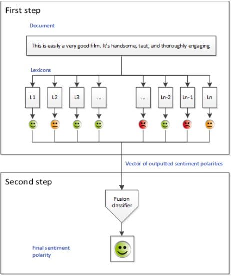
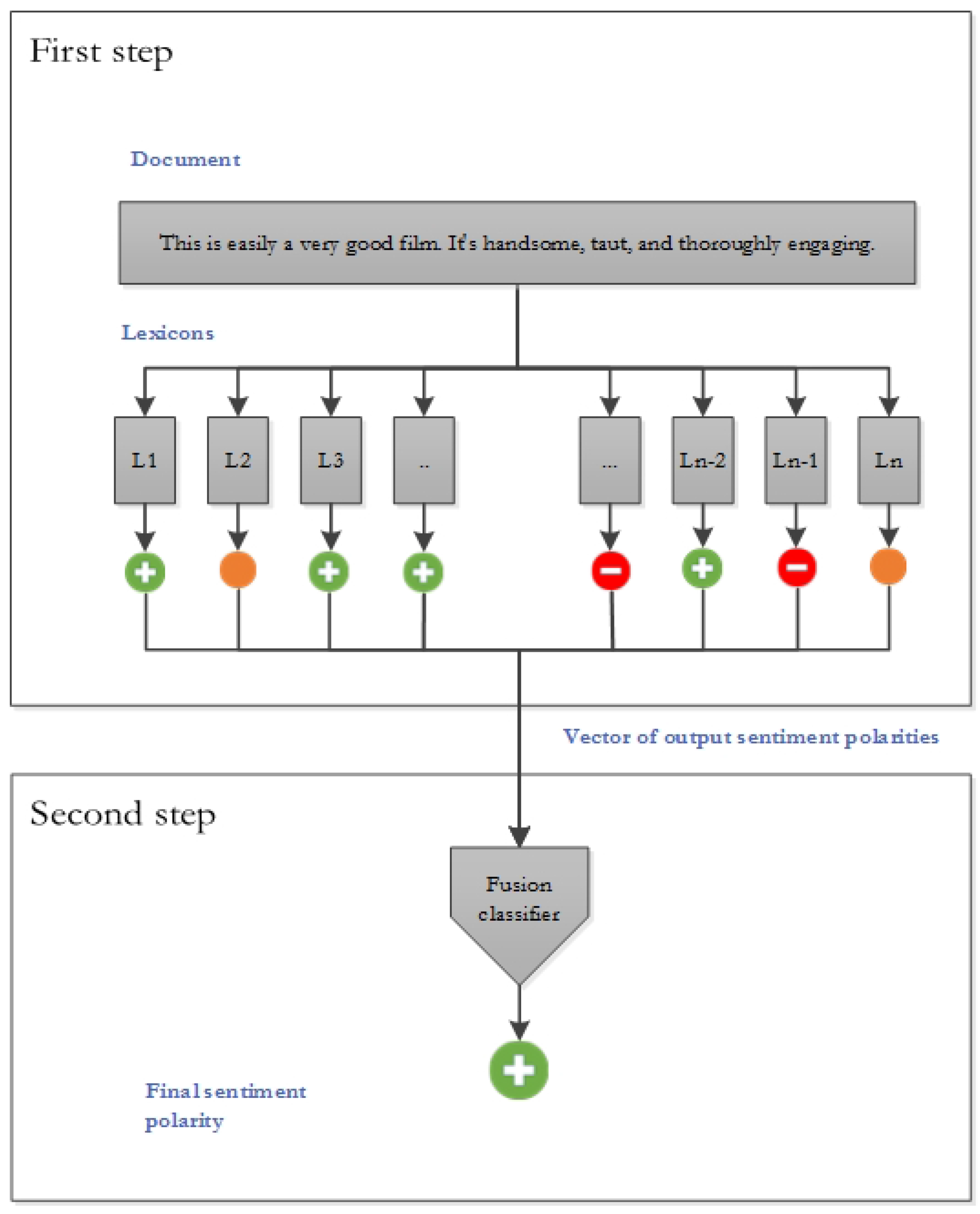
1.3. Ensemble Classification Approach
1.4. Our Contribution
- (1)
- Exploitation of the impact of unigram/bigram/trigram regarding both frequency and likelihood on a corpus upon its sentiment yields better results than expert annotation.
- (2)
- Employment of ensemble techniques on multiple lexicon outputs for learning of sentiment annotation schemes yields results comparable to supervised methods but is more efficient.
2. Experiment Design
- (1)
- Lexicon-based annotation.
- (2)
- Frequentiment-based lexicon generation.
- (3)
- Ensemble classifiers with lexicon sentiment prediction as input features.
- (4)
- Supervised learning classifiers used for comparison purposes.
2.1. Dataset and Data Preparation
- Automotive product reviews (188,728 reviews)
- Book reviews (12,886,488 reviews)
- Clothing reviews (581,933 reviews)
- Electronics product reviews (1,241,778 reviews)
- Health product reviews (428,781 reviews)
- Movie TV reviews (7,850,072 reviews)
- Music reviews (6,396,350 reviews)
- Sports Outdoor product reviews (510,991 reviews)
- Toy Game reviews (435,996 reviews)
- Video Game reviews (463,669 reviews)

| Star Score | Sentiment Class |
|---|---|
 | Negative |
| | Negative |
| | Neutral |
| | Positive |
| | Positive |
2.2. Sentiment Lexicons
| Lexicon | Positive Words | Negative Words |
|---|---|---|
| Simplest (SM) | good | bad |
| Simple List (SL) | good, awesome, great, fantastic, wonderful | bad, terrible, worst, sucks, awful, dumb |
| Simple List Plus (SL+) | good, awesome, great, fantastic, wonderful, best, love, excellent | bad, terrible, worst, sucks, awful, dumb, waist, boring, worse |
| Past and Future (PF) | will, has, must, is | was, would, had, were |
| Past and Future Plus (PF+) | will, has, must, is, good, awesome, great, fantastic, wonderful, best, love, excellent | was, would, had, were, bad, terrible, worst, sucks, awful, dumb, waist, boring, worse |
| Bing Liu | 2006 words | 4783 words |
| AFINN-96 | 516 words | 965 words |
| AFINN-111 | 878 words | 1599 words |
| enchantedlearning.com | 266 words | 225 words |
| MPAA | 2721 words | 4915 words |
| NRC Emotion | 2312 words | 3324 words |
3. Proposed Methods
- (1)
- Frequentiment lexicon generation (unigram, bigram and trigram lexicons are generated).
- (2)
- Ensemble classification (fusion classifier) step.
3.1. Novel Frequentiment-based Lexicon Generation
3.2. Ensembles of Weak Classifiers
4. Baselines
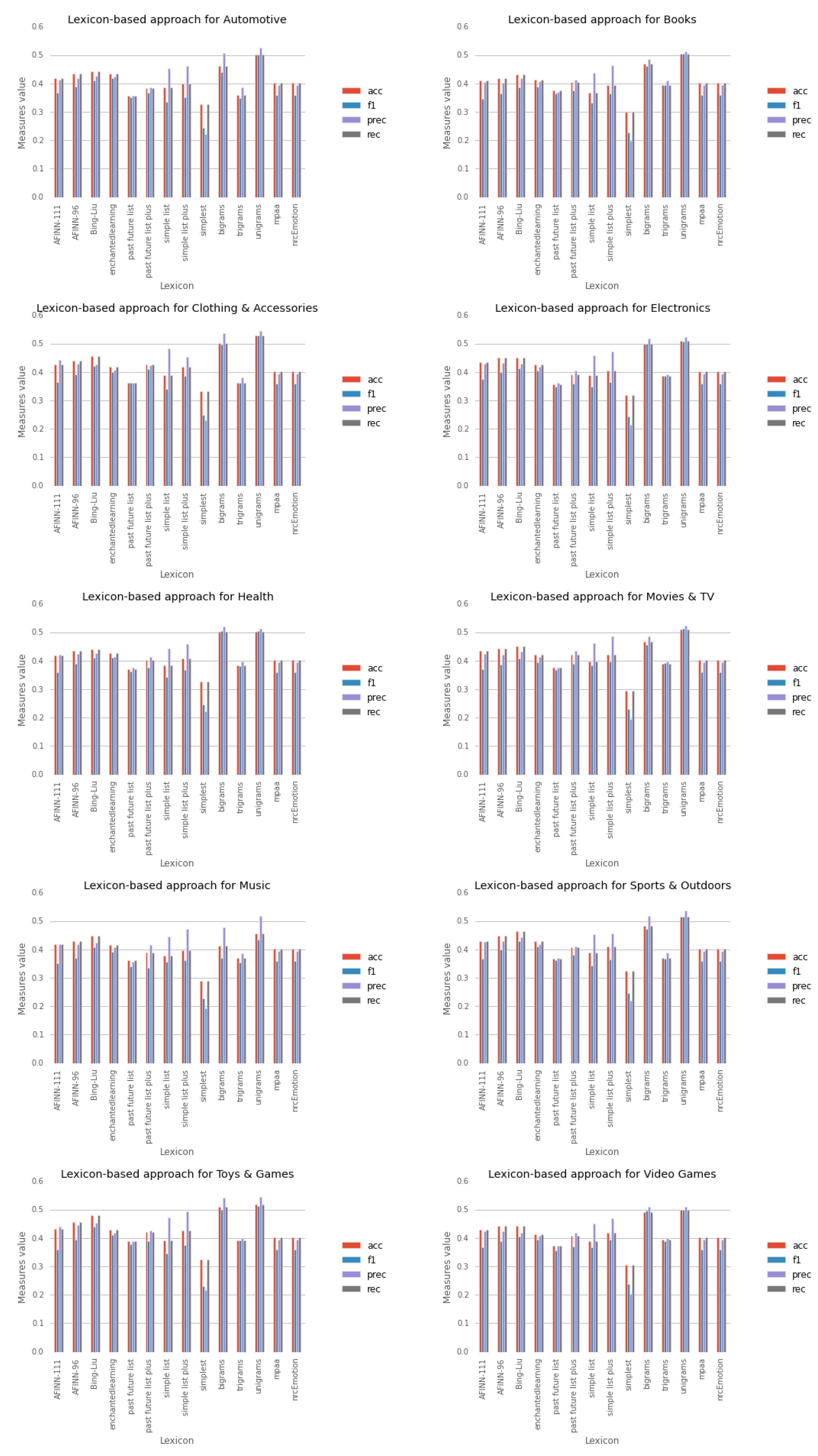
4.1. Semantic Orientation Lexicons
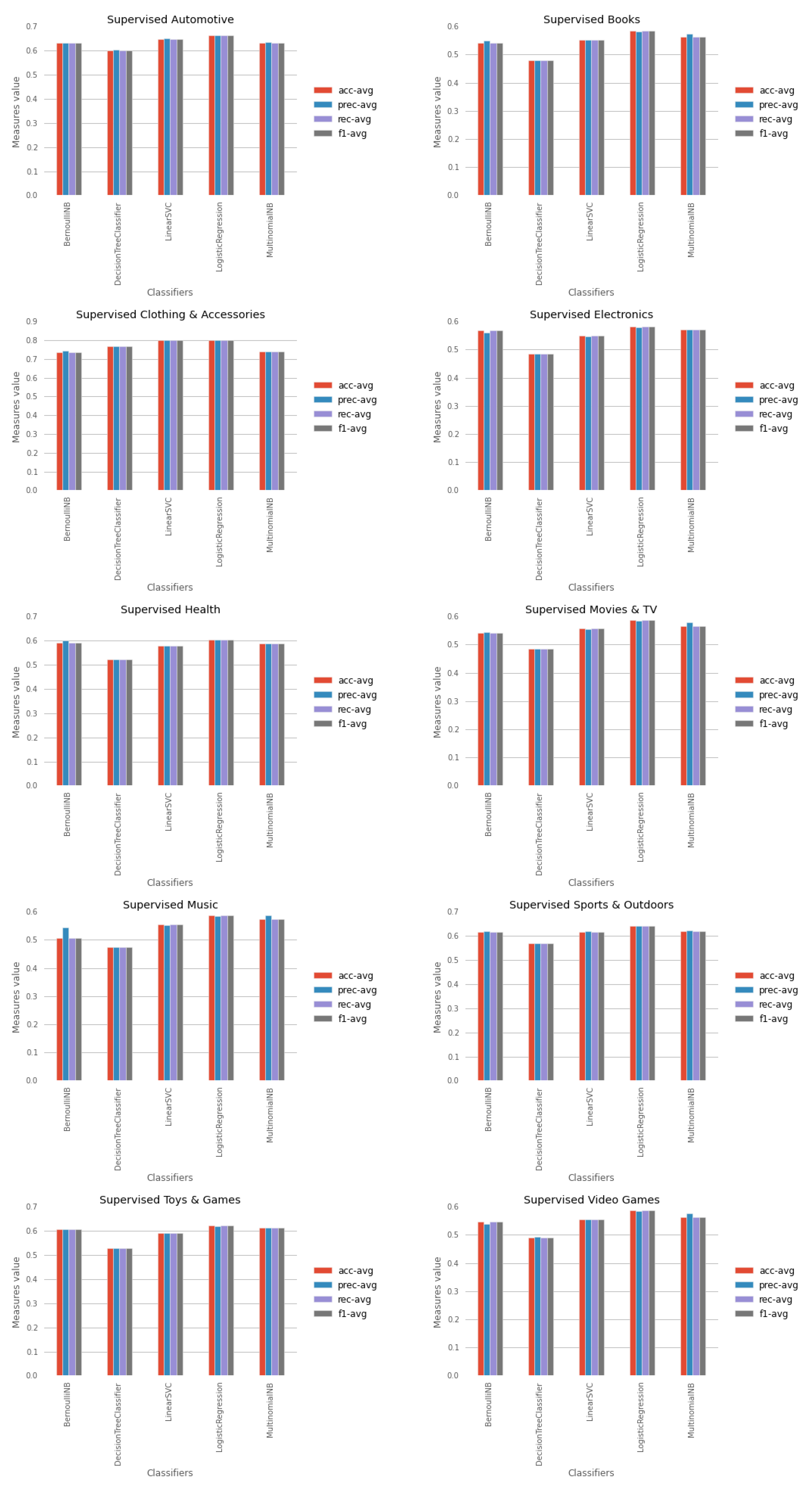
4.2. Supervised Learning Baseline
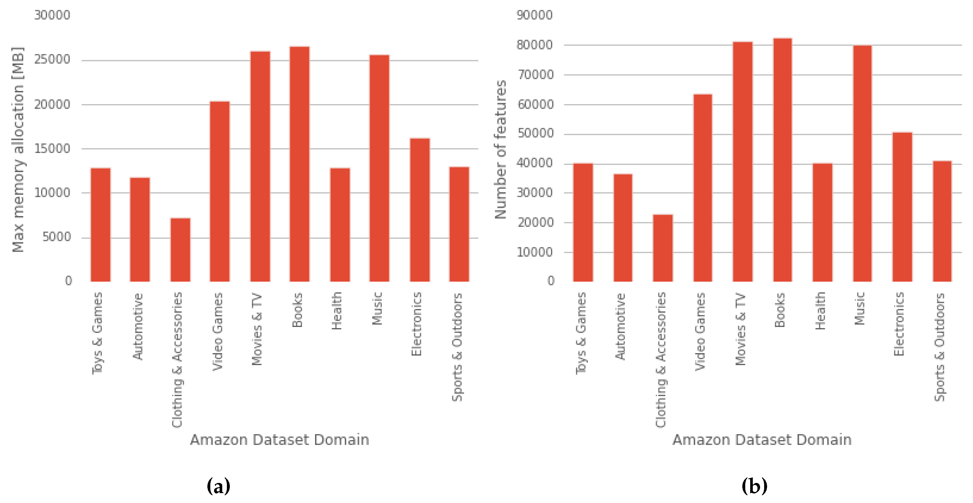
- Automotive: 36,789,
- Books: 82,541,
- Clothing & Accessories: 22,872,
- Electronics: 50,758,
- Health: 40,330,
- Movies & TV: 81,380,
- Music: 79,969,
- Sports & Outdoors: 40,956,
- Toys & Games: 40,253,
- Video Games: 63,471.
5. Results
| Method | Auto | Books | C&A | Elect | Health | M&TV | Mus | SP | T&G | VG | |
|---|---|---|---|---|---|---|---|---|---|---|---|
| Lexicon-based approach | SM | 0.244 | 0.227 | 0.249 | 0.244 | 0.245 | 0.230 | 0.228 | 0.245 | 0.230 | 0.237 |
| SL | 0.335 | 0.333 | 0.341 | 0.349 | 0.342 | 0.382 | 0.357 | 0.343 | 0.344 | 0.367 | |
| Emotion | 0.342 | 0.355 | 0.360 | 0.354 | 0.347 | 0.366 | 0.352 | 0.358 | 0.350 | 0.359 | |
| PF | 0.352 | 0.365 | 0.361 | 0.348 | 0.362 | 0.368 | 0.340 | 0.362 | 0.379 | 0.357 | |
| SL+ | 0.351 | 0.364 | 0.385 | 0.364 | 0.366 | 0.398 | 0.362 | 0.366 | 0.376 | 0.395 | |
| AF-111 | 0.368 | 0.346 | 0.364 | 0.376 | 0.358 | 0.370 | 0.350 | 0.368 | 0.359 | 0.368 | |
| PF+ | 0.366 | 0.375 | 0.411 | 0.360 | 0.376 | 0.389 | 0.335 | 0.381 | 0.387 | 0.370 | |
| trigr. | 0.348 | 0.395 | 0.361 | 0.386 | 0.380 | 0.390 | 0.353 | 0.366 | 0.392 | 0.388 | |
| AF-96 | 0.390 | 0.364 | 0.391 | 0.401 | 0.387 | 0.385 | 0.371 | 0.398 | 0.395 | 0.388 | |
| EN | 0.419 | 0.389 | 0.400 | 0.406 | 0.411 | 0.394 | 0.391 | 0.410 | 0.411 | 0.394 | |
| MPAA | 0.386 | 0.380 | 0.406 | 0.392 | 0.381 | 0.391 | 0.374 | 0.403 | 0.404 | 0.383 | |
| BL | 0.411 | 0.387 | 0.421 | 0.414 | 0.410 | 0.406 | 0.407 | 0.429 | 0.439 | 0.404 | |
| bigr. | 0.440 | 0.461 | 0.496 | 0.498 | 0.503 | 0.457 | 0.370 | 0.472 | 0.500 | 0.495 | |
| unigr. | 0.500 | 0.505 | 0.530 | 0.508 | 0.505 | 0.512 | 0.435 | 0.514 | 0.511 | 0.499 | |
| Supervised learn | DT | 0.600 | 0.478 | 0.770 | 0.484 | 0.521 | 0.486 | 0.474 | 0.569 | 0.528 | 0.491 |
| BNB | 0.631 | 0.542 | 0.737 | 0.568 | 0.591 | 0.542 | 0.506 | 0.617 | 0.606 | 0.546 | |
| LinSVC | 0.647 | 0.552 | 0.799 | 0.549 | 0.577 | 0.557 | 0.554 | 0.617 | 0.590 | 0.554 | |
| MNB | 0.631 | 0.564 | 0.740 | 0.571 | 0.587 | 0.567 | 0.573 | 0.618 | 0.614 | 0.564 | |
| LogR | 0.664 | 0.584 | 0.800 | 0.581 | 0.604 | 0.587 | 0.587 | 0.640 | 0.621 | 0.586 | |
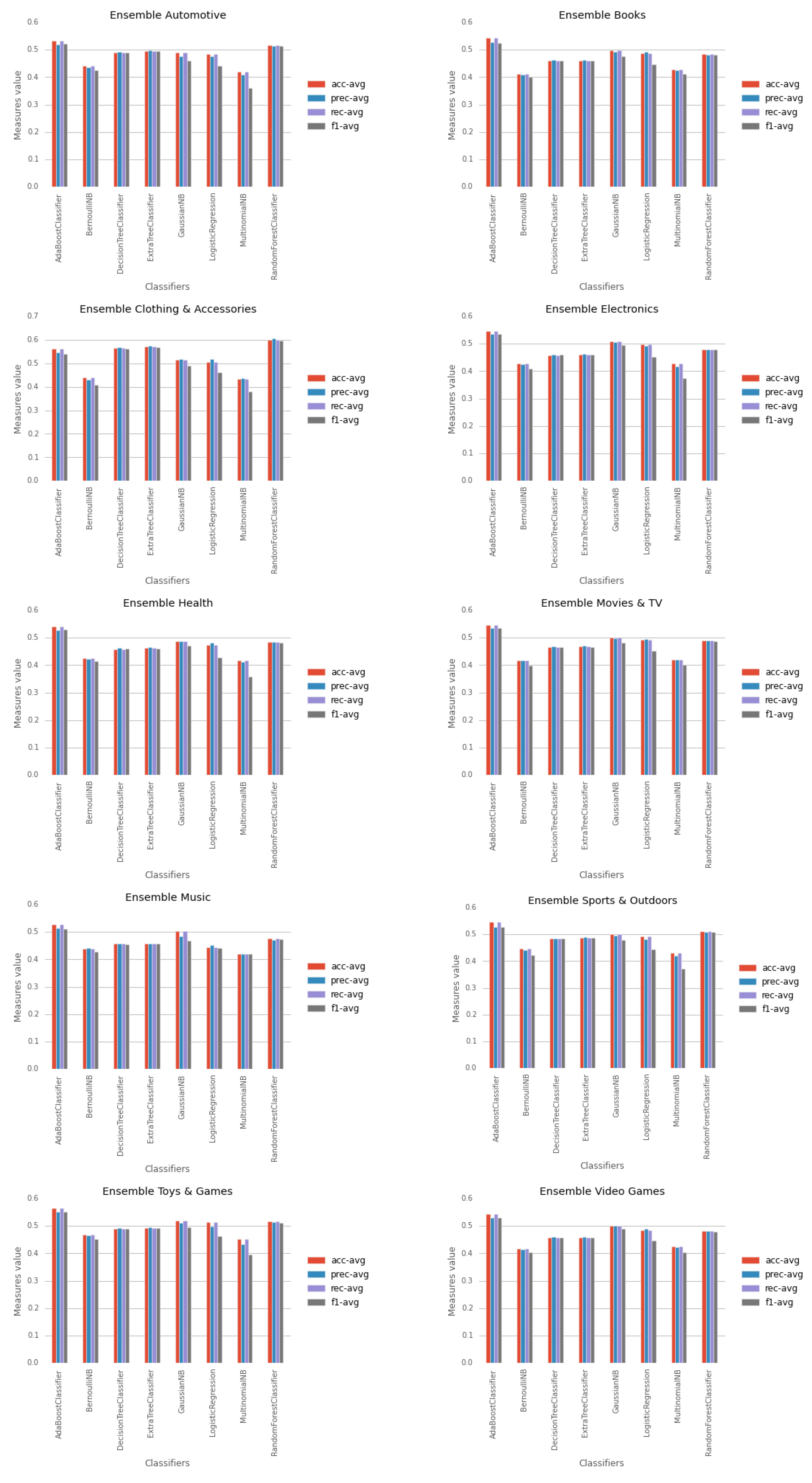
| Lexicon-based ensemble | NMB | 0.360 | 0.411 | 0.380 | 0.374 | 0.357 | 0.401 | 0.419 | 0.371 | 0.395 | 0.403 |
| BNB | 0.424 | 0.402 | 0.409 | 0.410 | 0.416 | 0.398 | 0.427 | 0.424 | 0.451 | 0.403 | |
| LogR | 0.441 | 0.448 | 0.461 | 0.451 | 0.428 | 0.453 | 0.441 | 0.444 | 0.463 | 0.446 | |
| DT | 0.491 | 0.460 | 0.562 | 0.459 | 0.459 | 0.465 | 0.456 | 0.484 | 0.490 | 0.457 | |
| GNB | 0.460 | 0.477 | 0.490 | 0.494 | 0.472 | 0.482 | 0.468 | 0.479 | 0.494 | 0.489 | |
| ET | 0.495 | 0.461 | 0.568 | 0.460 | 0.461 | 0.467 | 0.457 | 0.487 | 0.493 | 0.459 | |
| RF | 0.513 | 0.482 | 0.596 | 0.479 | 0.482 | 0.488 | 0.473 | 0.508 | 0.512 | 0.480 | |
| AB | 0.521 | 0.525 | 0.540 | 0.536 | 0.529 | 0.535 | 0.510 | 0.528 | 0.552 | 0.530 | |
| AVG | 0.449 | 0.431 | 0.494 | 0.438 | 0.439 | 0.439 | 0.421 | 0.452 | 0.455 | 0.437 |
- (1)
- Parameter estimation for the frequentiment lexicon generation.
- (2)
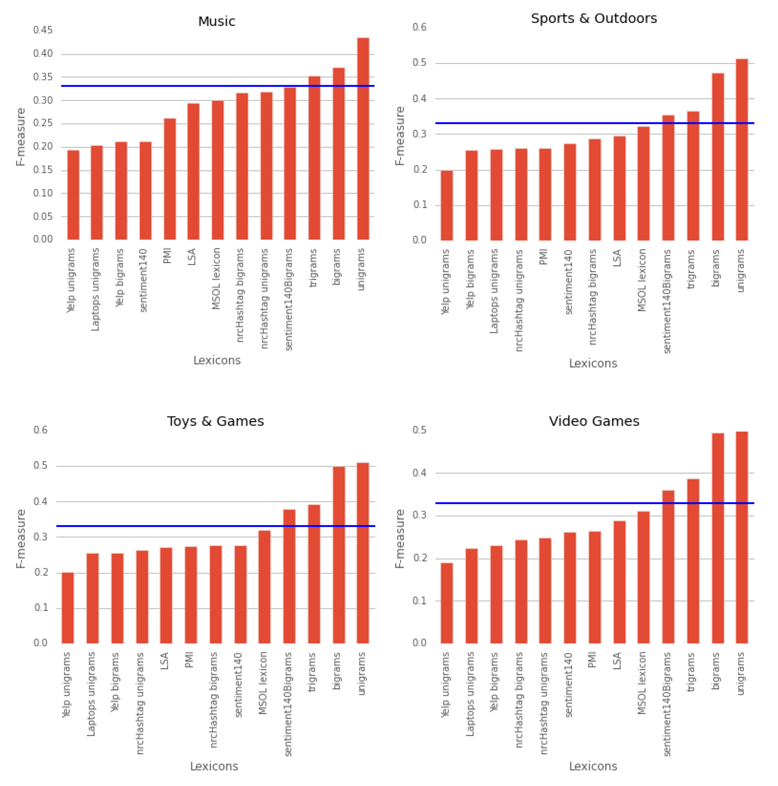
- Lexicon performance, frequentiment-generated versus state-of-the-art lexicons.
- (3)
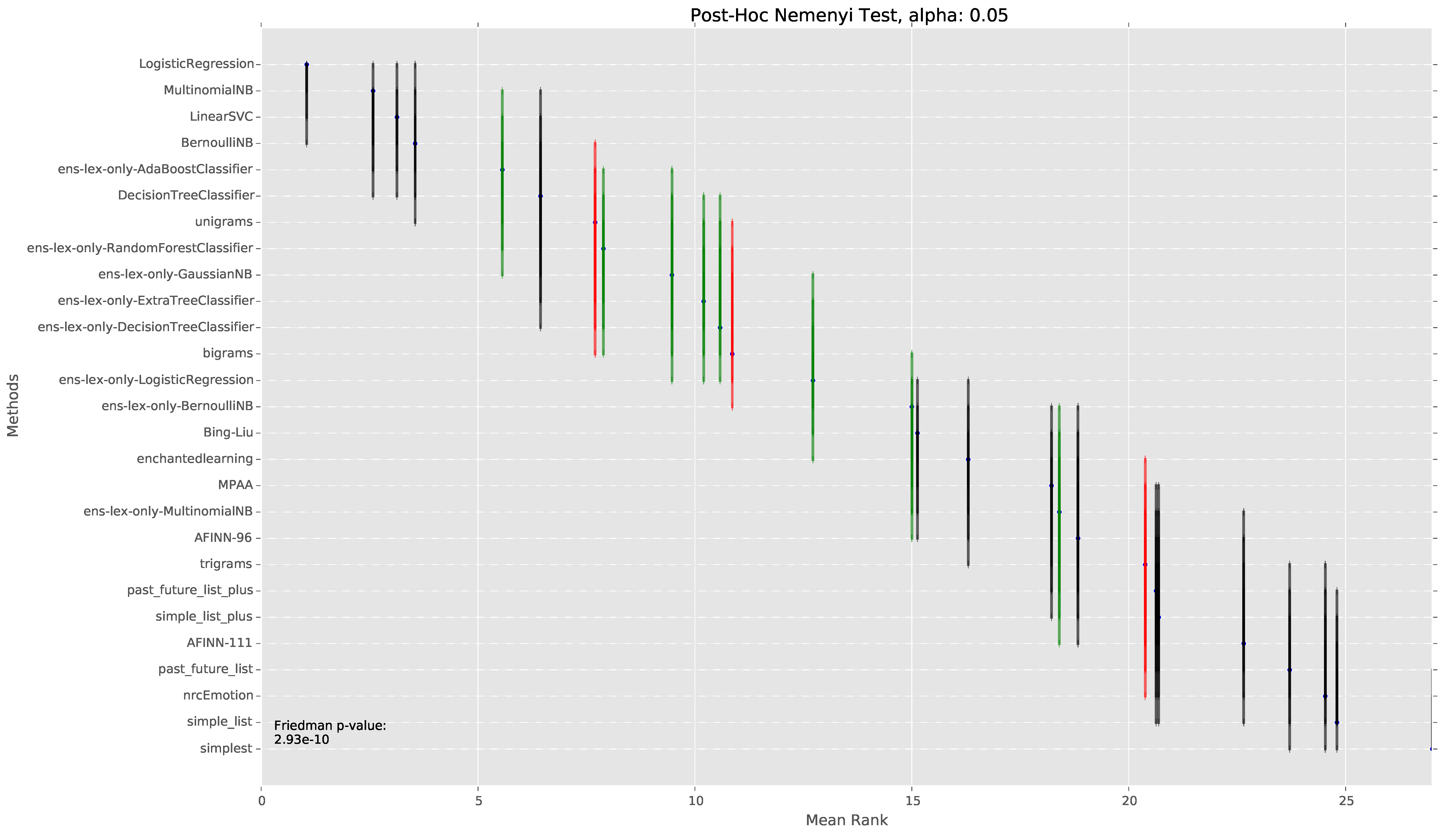
- Lexicon and lexicon-based ensemble methods compared to supervised learners.
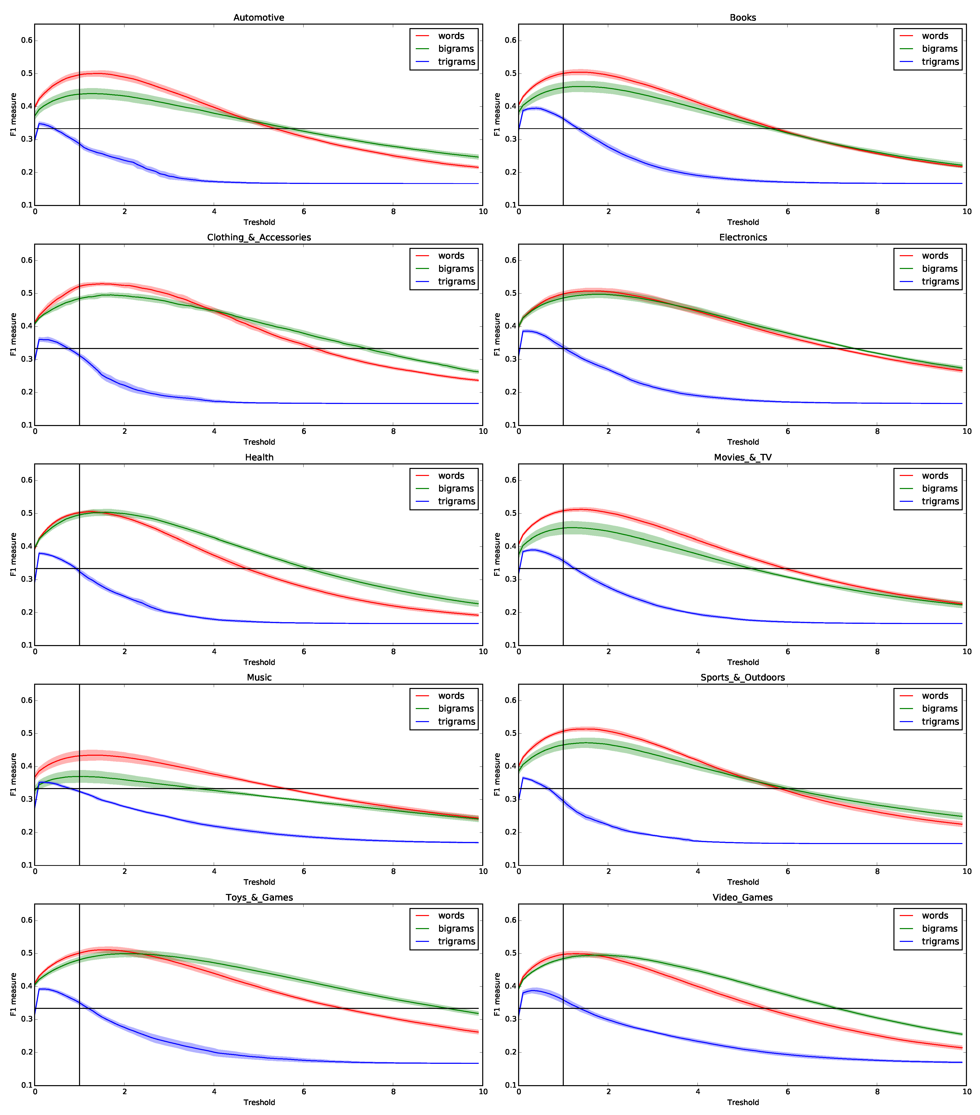
5.1. Parameter Estimation for Frequentiment Lexicon Generation
| Unigrams | Bigrams | Trigrams | |
|---|---|---|---|
| Automotive | 0.500 ± 0.008 | 0.440 ± 0.015 | 0.348 ± 0.005 |
| Books | 0.505 ± 0.008 | 0.461 ± 0.016 | 0.395 ± 0.005 |
| Clothing & Accessories | 0.530 ± 0.005 | 0.496 ± 0.007 | 0.361 ± 0.006 |
| Electronics | 0.508 ± 0.008 | 0.498 ± 0.010 | 0.386 ± 0.004 |
| Health | 0.505 ± 0.004 | 0.503 ± 0.009 | 0.380 ± 0.003 |
| Movies & TV | 0.512 ± 0.005 | 0.457 ± 0.019 | 0.390 ± 0.004 |
| Music | 0.435 ± 0.015 | 0.370 ± 0.018 | 0.353 ± 0.003 |
| Sports & Outdoors | 0.514 ± 0.006 | 0.472 ± 0.014 | 0.366 ± 0.003 |
| Toys & Games | 0.511 ± 0.008 | 0.500 ± 0.010 | 0.392 ± 0.004 |
| Video Games | 0.499 ± 0.007 | 0.495 ± 0.005 | 0.388 ± 0.007 |
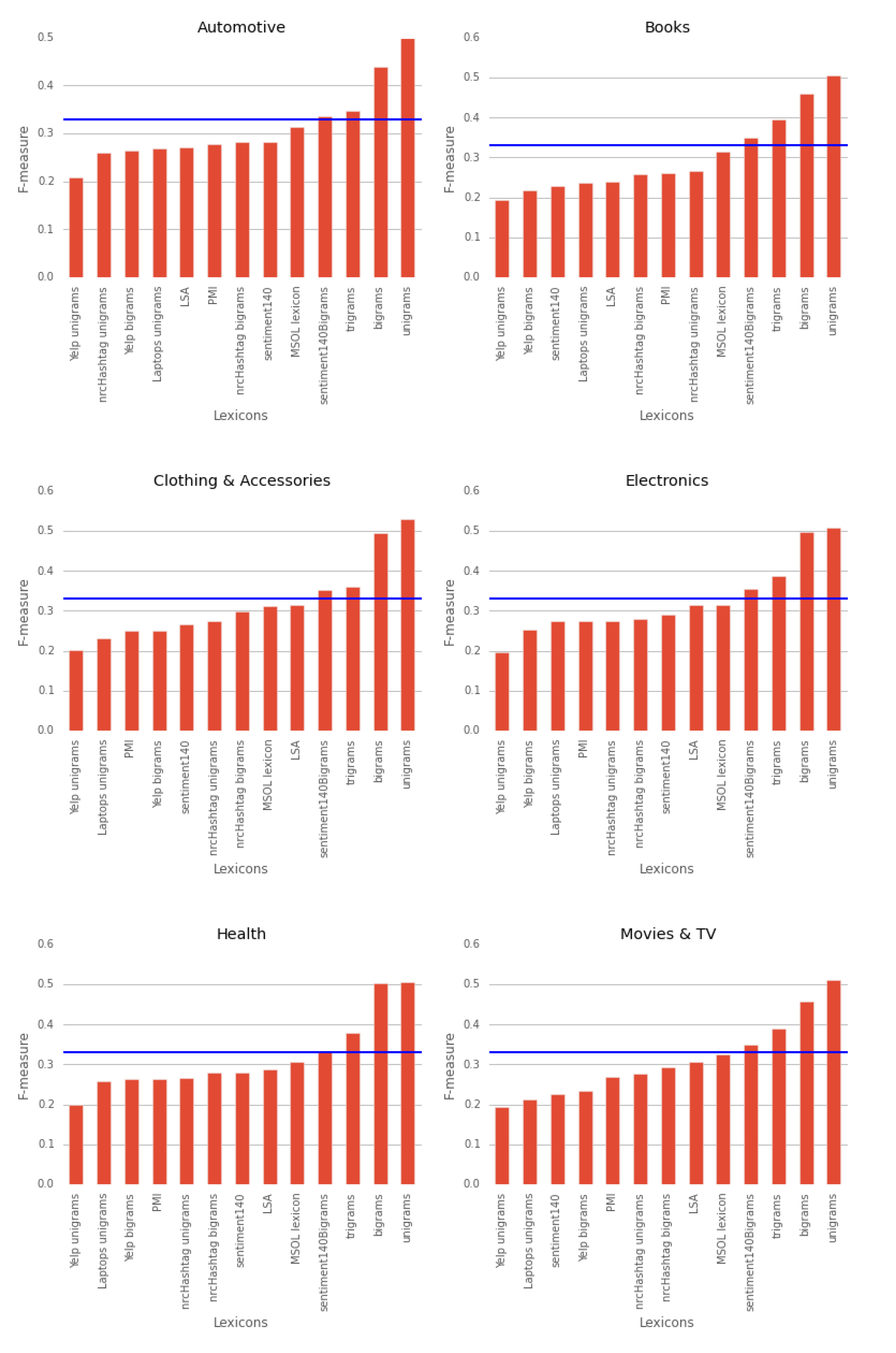
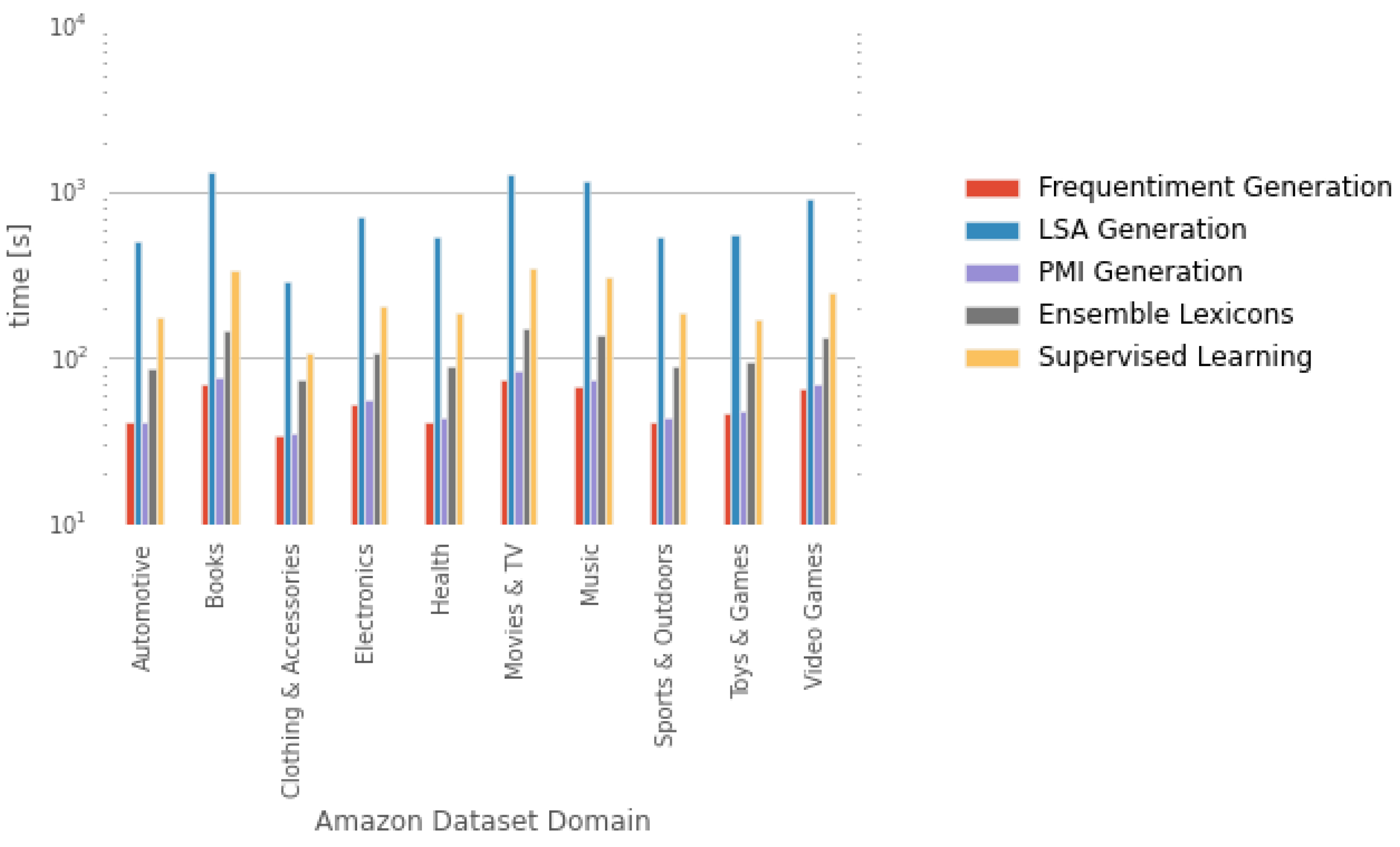
5.2. Frequentiment Lexicon Performance and Characteristics
| Unigrams | Bigrams | Trigrams | |
|---|---|---|---|
| Automotive | 372.1 ± 4.3 | 536.2 ± 6.7 | 52.5 ± 1.7 |
| Books | 641.7 ± 10.7 | 877.3 ± 14.2 | 140.5 ± 5.0 |
| Clothing & Accessories | 290.6 ± 4.0 | 531.8 ± 6.6 | 63.8 ± 2.4 |
| Electronics | 514.2 ± 7.7 | 727.3 ± 11.8 | 95.1 ± 4.3 |
| Health | 356.9 ± 5.8 | 563.0 ± 5.7 | 68.8 ± 1.4 |
| Movies & TV | 660.9 ± 3.6 | 896.7 ± 7.2 | 137.6 ± 2.7 |
| Music | 548.6 ± 5.1 | 817.0 ± 14.1 | 121.3 ± 4.3 |
| Sports & Outdoors | 362.2 ± 5.2 | 552.0 ± 6.9 | 62.0 ± 3.3 |
| Toys & Games | 379.4 ± 5.2 | 682.7 ± 7.5 | 98.4 ± 2.7 |
| Video Games | 549.4 ± 9.9 | 935.4 ± 8.5 | 171.3 ± 4.0 |
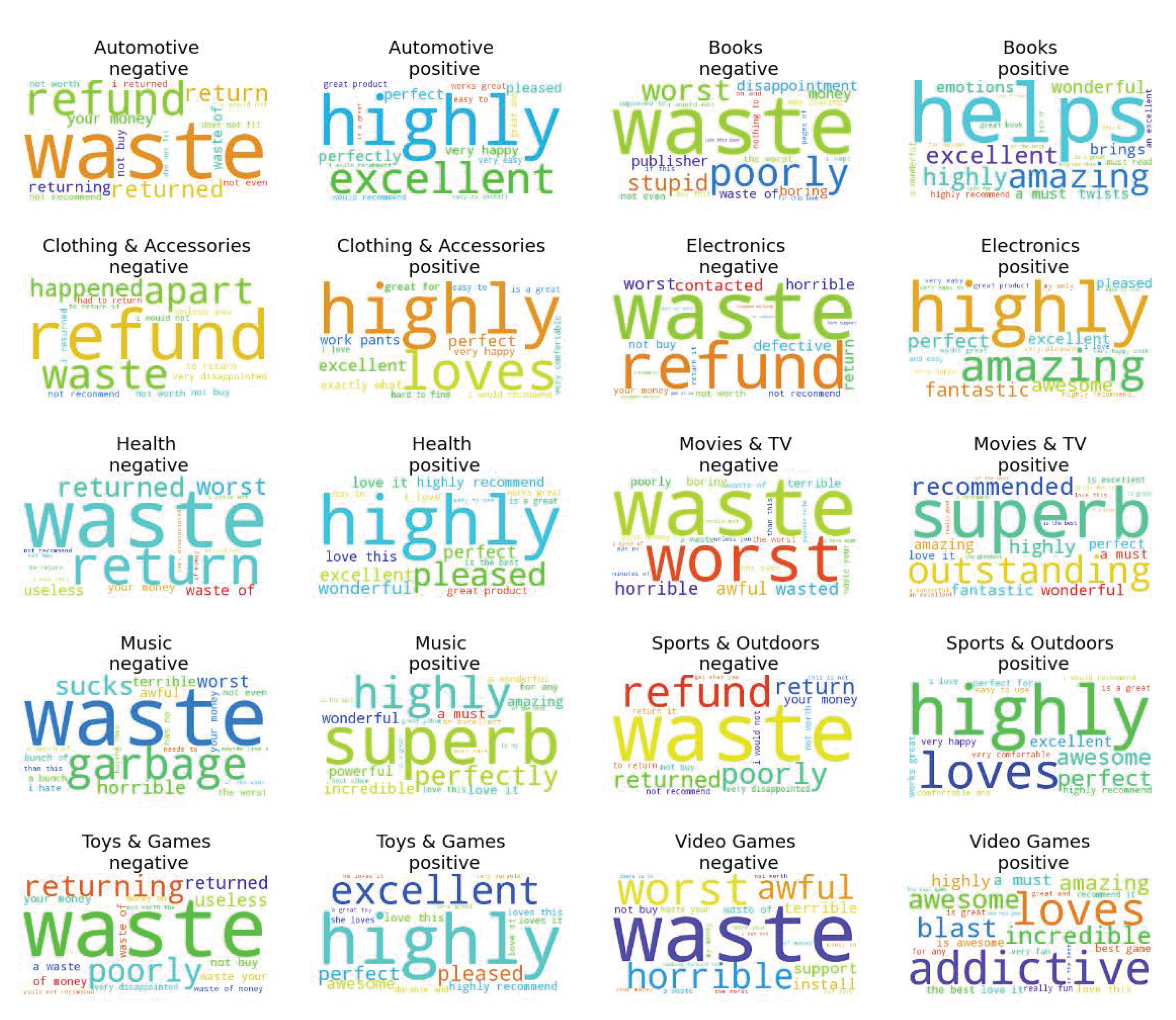
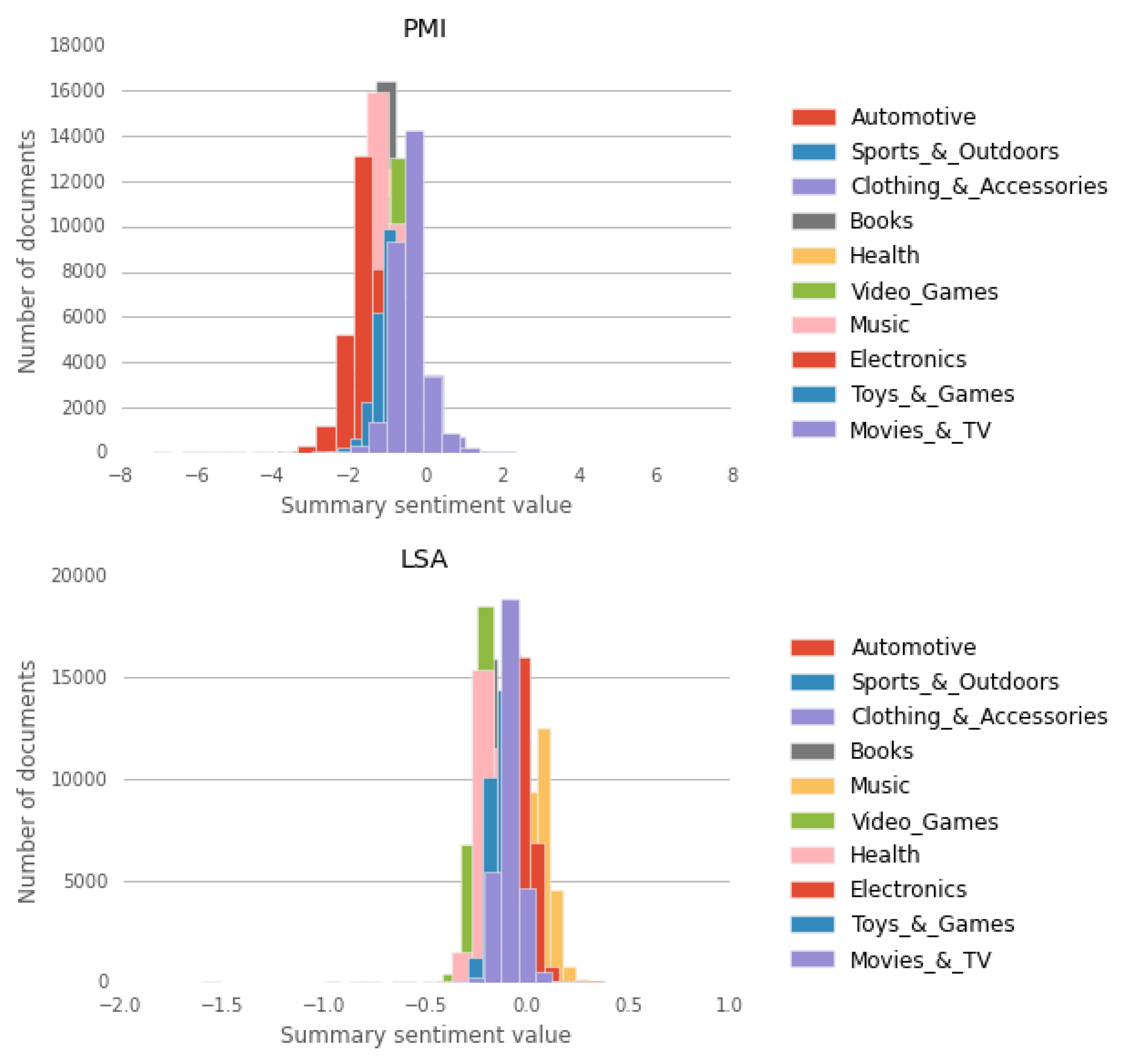
5.2.1. Analysis of the Most Prominent Lexicon Features
5.2.2. Lexicon-based Approach Evaluation
5.2.3. Underperforming Lexicons
5.3. Comparison Between Domains
Computational Complexity
6. Discussion
| Unigrams | Bigrams | Trigrams | |
|---|---|---|---|
| Automotive | 1.4 | 1.3 | 0.1 |
| Books | 1.4 | 1.3 | 0.4 |
| Clothing & Accessories | 1.5 | 1.7 | 0.1 |
| Electronics | 1.7 | 1.8 | 0.1 |
| Health | 1.2 | 1.6 | 0.1 |
| Movies & TV | 1.4 | 1.2 | 0.3 |
| Music | 1.4 | 1.1 | 0.2 |
| Sports & Outdoors | 1.5 | 1.5 | 0.1 |
| Toys & Games | 1.5 | 2 | 0.2 |
| Video Games | 1.3 | 1.9 | 0.3 |
| Avg ± Std | 1.43 ± 0.13 | 1.54 ± 0.29 | 0.19 ± 0.10 |
7. Conclusions and Future Work
Acknowledgments
Author Contributions
Conflicts of Interest
References
- Tumasjan, A.; Sprenger, T.O.; Sandner, P.G.; Welpe, I.M. Predicting Elections with Twitter: What 140 Characters Reveal about Political Sentiment. ICWSM 2010, 10, 178–185. [Google Scholar]
- Ghiassi, M.; Skinner, J.; Zimbra, D. Twitter brand sentiment analysis: A hybrid system using n-gram analysis and dynamic artificial neural network. Expert Syst. Appl. 2013, 40, 6266–6282. [Google Scholar] [CrossRef]
- Brody, S.; Elhadad, N. An Unsupervised Aspect-sentiment Model for Online Reviews. In Proceedings of Human Language Technologies: The 2010 Annual Conference of the North American Chapter of the ACL, Los Angeles, CA, USA, 1–6 June 2010; pp. 804–812.
- Bollen, J.; Mao, H.; Zeng, X. Twitter mood predicts the stock market. J. Comput. Sci. 2011, 2, 1–8. [Google Scholar] [CrossRef]
- Liu, B.; Zhang, L. A Survey of Opinion Mining and Sentiment Analysis. In Mining Text Data; Springer-Verlag: New York, NY, USA, 2012; pp. 415–463. [Google Scholar]
- Pang, B.; Lee, L. Opinion mining and sentiment analysis. Found. Trends Inf. Retr. 2008, 2, 1–135. [Google Scholar] [CrossRef]
- Medhat, W.; Hassan, A.; Korashy, H. Sentiment analysis algorithms and applications: A survey. Ain Shams Eng. J. 2014, 5, 1093–1113. [Google Scholar] [CrossRef]
- Liu, B. Sentiment Analysis and Opinion Mining. In Proceedings of the Twenty-Fifth Conference on Artificial Intelligence (AAAI-11), San Francisco, CA, USA, 7–11 August 2011.
- Hu, M.; Liu, B. Mining and Summarizing Customer Reviews. In Proceedings of the Tenth ACM SIGKDD International Conference on Knowledge Discovery and Data Mining, Seattle, WA, USA, 22–25 August 2004; ACM: New York, NY, USA, 2004; pp. 168–177. [Google Scholar]
- Qiu, G.; Liu, B.; Bu, J.; Chen, C. Expanding Domain Sentiment Lexicon Through Double Propagation. In Proceedings of the 21st International Jont Conference on Artifical Intelligence (IJCAI’09), Pasadena, CA, USA, 11–17 July 2009; Morgan Kaufmann Publishers Inc.: San Francisco, CA, USA, 2009; pp. 1199–1204. [Google Scholar]
- Hatzivassiloglou, V.; McKeown, K.R. Predicting the semantic orientation of adjectives. In Proceedings of the 35th Annual Meeting of the Association for Computational Linguistics and 8th Conference of the European Chapter of the Association for Computational Linguistics, Madrid, Spain, 7–12 July 1997; pp. 174–181.
- Yu, H.; Hatzivassiloglou, V. Towards Answering Opinion Questions: Separating Facts from Opinions and Identifying the Polarity of Opinion Sentences. In Proceedings of the 2003 Conference on Empirical Methods in Natural Language Processing (EMNLP’03), Sapporo, Japan, 11–12 July 2003; Association for Computational Linguistics: Stroudsburg, PA, USA, 2003; pp. 129–136. [Google Scholar]
- Read, J.; Carroll, J. Weakly supervised techniques for domain-independent sentiment classification. In Proceedings of the 1st International CIKM Workshop on Topic-Sentiment Analysis for Mass Opinion, Hong Kong, China, 6 November 2009; ACM: New York, NY, USA, 2009; pp. 45–52. [Google Scholar]
- Whitehead, M.; Yaeger, L. Sentiment mining using ensemble classification models. In Innovations and Advances in Computer Sciences and Engineering; Springer Netherlands: Dordrecht, The Netherlands, 2010; pp. 509–514. [Google Scholar]
- Lu, Y.; Castellanos, M.; Dayal, U.; Zhai, C. Automatic Construction of a Context-aware Sentiment Lexicon: An Optimization Approach. In Proceedings of the 20th International Conference on World Wide Web (WWW’11), Hyderabad, India, 30 March 2011; ACM: New York, NY, USA, 2011; pp. 347–356. [Google Scholar]
- Ding, X.; Liu, B.; Yu, P.S. A Holistic Lexicon-based Approach to Opinion Mining. In Proceedings of the 2008 International Conference on Web Search and Data Mining (WSDM’08), Palo Alto, CA, USA, 11–12 February 2008; ACM: New York, NY, USA, 2008; pp. 231–240. [Google Scholar]
- Mohammad, S.M.; Kiritchenko, S.; Zhu, X. NRC-Canada: Building the State-of-the-Art in Sentiment Analysis of Tweets. In Proceedings of the Seventh International Workshop on Semantic Evaluation Exercises (SemEval-2013), Atlanta, GA, USA, 14–15 June 2013; Association for Computational Linguistics: Stroudsburg, PA, USA, 2013; pp. 321–327. [Google Scholar]
- Weiss, S.M.; Kulikowski, C.A. Computer Systems That Learn: Classification and Prediction Methods from Statistics, Neural Nets, Machine Learning, and Expert Systems; Morgan Kaufmann Publishers Inc.: San Francisco, CA, USA, 1991. [Google Scholar]
- Bo, P.; Lillian, L.; Shivakumar, V. Thumbs up?: Sentiment classification using machine learning techniques. In Proceedings of the ACL-02 Conference on Empirical Methods in Natural Language Processing, Philadelphia, PA, USA, 6–7 July 2002; Association for Computational Linguistics: Stroudsburg, PA, USA, 2002; Volume 10, pp. 79–86. [Google Scholar]
- Ye, Q.; Zhang, Z.; Law, R. Sentiment classification of online reviews to travel destinations by supervised machine learning approaches. Expert Syst. Appl. 2009, 36, 6527–6535. [Google Scholar] [CrossRef]
- Schler, J. The Importance of Neutral Examples for Learning Sentiment. In Proceedings of the Workshop on the Analysis of Informal and Formal Information Exchange during Negotiations (FINEXIN05), Ottawa, ON, Canada, 26–27 May 2005.
- Bai, X. Predicting consumer sentiments from online text. Decis. Support Syst. 2011, 50, 732–742. [Google Scholar] [CrossRef]
- Socher, R.; Perelygin, A.; Wu, J.Y.; Chuang, J.; Manning, C.D.; Ng, A.Y.; Potts, C. Recursive deep models for semantic compositionality over a sentiment treebank. In Proceedings of the Conference on Empirical Methods in Natural Language Processing (EMNLP 2013), Seattle, WA, USA, 18–21 October 2013; Volume 1631, p. 1642.
- Narayanan, V.; Arora, I.; Bhatia, A. Fast and Accurate Sentiment Classification Using an Enhanced Naive Bayes Model. In Proceedings of the 14th International Conference on Intelligent Data Engineering and Automated Learning (IDEAL 2013), Hefei, China, 20–23 October 2013; Volume 8206, pp. 194–201.
- Gamon, M. Sentiment Classification on Customer Feedback Data: Noisy Data, Large Feature Vectors, and the Role of Linguistic Analysis. In Proceedings of the 20th International Conference on Computational Linguistics (COLING’04), Geneva, Switzerland,, 23–27 August 2004; Association for Computational Linguistics: Stroudsburg, PA, USA, 2004. [Google Scholar]
- Augustyniak, L.; Kajdanowicz, T.; Kazienko, P.; Kulisiewicz, M.; Tuliglowicz, W. An Approach to Sentiment Analysis of Movie Reviews: Lexicon Based vs.. Classification. In Proceedings of the 9th International Conference on Hybrid Artificial Intelligence Systems (HAIS 2014), Salamanca, Spain, 11–13 June 2014; pp. 168–178.
- Augustyniak, L.; Kajdanowicz, T.; Szymanski, P.; Tuliglowicz, W.; Kazienko, P.; Alhajj, R.; Szymanski, B.K. Simpler is better? Lexicon-based ensemble sentiment classification beats supervised methods. In Proceedings of the 2014 IEEE/ACM International Conference on Advances in Social Networks Analysis and Mining (ASONAM 2014), Beijing, China, 17–20 August 2014; pp. 924–929.
- Whitehead, M.; Yaeger, L. Sentiment Mining Using Ensemble Classification Models. In Innovations and Advances in Computer Sciences and Engineering; Springer Netherlands: Dordrecht, The Netherlands, 2010; pp. 509–514. [Google Scholar]
- Breiman, L. Bagging Predictors. Mach. Learn. 1996, 24, 123–140. [Google Scholar] [CrossRef]
- Schapire, R.E. A Brief Introduction to Boosting. In Proceedings of the 16th International Joint Conference on Artificial Intelligence (IJCAI 99), Stockholm, Sweden, 31 July–6 August 1999; pp. 1401–1406.
- Polikar, R. Ensemble Based Systems in Decision Making. IEEE Circ. Syst. Mag. 2006, 6, 21–45. [Google Scholar] [CrossRef]
- McAuley, J.; Leskovec, J. Hidden factors and hidden topics: understanding rating dimensions with review text. In Proceedings of the 7th ACM Conference on Recommender Systems, Hong Kong, China, 12–16 October 2013; ACM: New York, NY, USA, 2013; pp. 165–172. [Google Scholar]
- Python Library Beautiful Soup. Available online: https://pypi.python.org/pypi/beautifulsoup4 (accessed on 1 February 2015).
- Python Library Unidecode. Available online: https://pypi.python.org/pypi/Unidecode (accessed on 1 February 2015).
- Turney, P.D.; Littman, M.L. Measuring Praise and Criticism: Inference of Semantic Orientation from Association. ACM Trans. Inf. Syst. 2003, 21, 315–346. [Google Scholar] [CrossRef]
- Nielsen, F.Å. AFINN Informatics and Mathematical Modelling, Technical University of Denmark, 2011. Available online: http://www2.imm.dtu.dk/pubdb/p.php?6010 (accessed on 24 December 2015).
- Wilson, T.; Wiebe, J.; Hoffmann, P. Recognizing Contextual Polarity in Phrase-level Sentiment Analysis. In Proceedings of the Conference on Human Language Technology and Empirical Methods in Natural Language Processing, Vancouver, BC, Canada, 6–8 October 2005; Association for Computational Linguistics: Stroudsburg, PA, USA, 2005; pp. 347–354. [Google Scholar]
- Mohammad, S.M.; Turney, P.D. Crowdsourcing a Word-Emotion Association Lexicon. Comput. Intell. 2013, 29, 436–465. [Google Scholar] [CrossRef]
- Kiritchenko, S.; Zhu, X.; Cherry, C.; Mohammad, S. NRC-Canada-2014: Detecting Aspects and Sentiment in Customer Reviews. In Proceedings of the 8th International Workshop on Semantic Evaluation (SemEval 2014), Dublin, Ireland, 23–24 August 2014; Association for Computational Linguistics and Dublin City University: Dublin, Ireland, 2014; pp. 437–442. [Google Scholar]
- Turney, P.D.; Littman, M.L. Measuring praise and criticism: Inference of semantic orientation from association. ACM Trans. Inf. Syst. 2003, 21, 315–346. [Google Scholar] [CrossRef]
- SemEval Contest Website. Available online: https://www.cs.york.ac.uk/semeval-2013/task2 (accessed on 1 March 2015).
- Cieliebak, M.; Dürr, O.; Uzdilli, F. Meta-Classifiers Easily Improve Commercial Sentiment Detection Tools. In Proceedings of the 9th International Conference on Language Resources and Evaluation (LREC’14), Reykjavik, Iceland, 26–31 May 2014; European Language Resources Association (ELRA): Reykjavik, Iceland, 2014. [Google Scholar]
- NRC Canada Website. Available online: http://saifmohammad.com/WebPages/lexicons.html (accessed on 1 August 2015).
- Macquarie Semantic Orientation Lexicon (MSOL) Link. Available online: http://www.saifmohammad.com/Release/MSOL-June15-09.txt (accessed on 1 August 2015).
- Higher-level threading interface in Python. Available online: https://docs.python.org/2/library/threading.html (accessed on 1 February 2015).
- Python Library Memory Profiler. Available online: https://pypi.python.org/pypi/memory/profiler (accessed on 1 August 2015).
- Tang, D.; Wei, F.; Qin, B.; Zhou, M.; Liu, T. Building Large-Scale Twitter-Specific Sentiment Lexicon:A Representation Learning Approach. In Proceedings of the 25th International Conference on Computational Linguistics (COLING 2014), Dublin, Ireland, 23–29 August 2014; Dublin City University and Association for Computational Linguistics: Dublin, Ireland, 2014; pp. 172–182. [Google Scholar]
© 2015 by the authors; licensee MDPI, Basel, Switzerland. This article is an open access article distributed under the terms and conditions of the Creative Commons by Attribution (CC-BY) license (http://creativecommons.org/licenses/by/4.0/).
Share and Cite
Augustyniak, Ł.; Szymański, P.; Kajdanowicz, T.; Tuligłowicz, W. Comprehensive Study on Lexicon-based Ensemble Classification Sentiment Analysis. Entropy 2016, 18, 4. https://doi.org/10.3390/e18010004
Augustyniak Ł, Szymański P, Kajdanowicz T, Tuligłowicz W. Comprehensive Study on Lexicon-based Ensemble Classification Sentiment Analysis. Entropy. 2016; 18(1):4. https://doi.org/10.3390/e18010004
Chicago/Turabian StyleAugustyniak, Łukasz, Piotr Szymański, Tomasz Kajdanowicz, and Włodzimierz Tuligłowicz. 2016. "Comprehensive Study on Lexicon-based Ensemble Classification Sentiment Analysis" Entropy 18, no. 1: 4. https://doi.org/10.3390/e18010004
APA StyleAugustyniak, Ł., Szymański, P., Kajdanowicz, T., & Tuligłowicz, W. (2016). Comprehensive Study on Lexicon-based Ensemble Classification Sentiment Analysis. Entropy, 18(1), 4. https://doi.org/10.3390/e18010004