1. Introduction
Along much of the 20th century, there had been many contributions to the development of a thermodynamic treatment of relativity and cosmology [
1–
3]: since the extension of thermodynamics to special relativity, first carried out by Planck [
4] and by Einstein [
5] and after to general relativity [
1], until the thermodynamic approaches to cosmology [
2,
3,
6].
On the other hand, Kaluza in 1921 [
7] and Klein in 1926 [
8] proposed a generalization of general relativity to unify gravitation and electromagnetism by using a five-dimensional geometrical model of space-time. Since then, many
n-dimensional models within cosmology have been proposed [
9–
19]. In 1989, Landsberg and de Vos [
20] made an
n-dimensional generalization of the Planck distribution, the Wien displacement law and the Stefan–Boltzmann law for black body radiation (BBR) within a zero curvature space. These authors also calculated the total internal energy
U of radiation filling a hypervolume
V leading to the recognition of the system as an ideal quantum gas obeying
pV =
εU,
p being the pressure and
ε a constant given by
. Recently, there has been great interest in systems satisfying this kind of equation of state with
ε positive or negative
for the case of an expanding accelerated universe [
21,
22]. Later, Menon and Agrawal [
23] modified the expression for the Stefan–Boltzmann constant in
n-dimensions found by Landsberg and De Vos by using the appropriate spin-degeneracy factor of the photon without affecting the curves of the normalized Planck spectrum found by Landsberg and De Vos. In 1990, Barrow and Hawthorne investigated the behavior of matter and radiation in thermal equilibrium in an
n-dimensional space in the early universe; in particular, they calculated the number of particles
N, the pressure
p and the energy density
u [
9]. In all of these cases, the results have to do with an isotropic and homogeneous average universe. Within this context, in the present paper, in addition to the Landsberg–de Vos and Barrow–Hawthorne results for BB-radiation in an
n-dimensional space, we calculate for this system the thermodynamic potentials, the efficiency of a Carnot cycle, the equation of adiabatic processes and the heat capacity at constant volume. By using Planck units, it is possible to find new and interesting information about the BBR thermodynamic potentials. A peculiar behavior in the potentials appear at very high temperatures and low dimensionality, suggesting that a cosmological approach of this phenomenon could give some clues about the nature of the dimensionality of our space. The need for understanding this aspect of our universe can be tracked to the ancient Greece [
24]. In modern times, this problem was first studied by Kant in 1746 [
25] and later, among others, by Ehrenfest in 1917 [
26], Barrow in 1983 [
24], Brandenberger and Vafa in 1989 [
6] and Tegmark in 1997 [
27] (see also [
19,
28–
30]).
On the other hand, some corrections have been proposed in the context of loop quantum gravity (LQG) by changing the dispersion relation of photons in an
n-dimensional flat space [
31]. Since the region of interest is the one with a very high temperature, we will incorporate these corrections to the dispersion relation and the Planck function in order to find the corresponding modification of the thermodynamic potentials.
The article is organized as follows: In Section 2, the generalization of the thermodynamic potentials, the pressure and the chemical potential to
n space dimensions is showed. In Section 3, the equation for adiabatic processes is found. In Section 4, the efficiency of a Carnot cycle is calculated. In Section 5, an analysis of critical points of the thermodynamic potentials is made, which suggests a possible application to cosmology, which is addressed in Section 6. In Section 7, a modification to the dispersion relation stemming from LQG theory is incorporated into the analysis. Finally, in Section 8, some conclusions are presented.
Appendices A and
B contain some mathematical calculations including the Carnot efficiency.
2. Generalization to n Dimensions
For a black body in an
n-dimensional space, it is known [
9,
20,
23,
32–
34] that the distribution of modes in the interval
ν to
ν +
dν is,
where V is the hypervolume,
n the dimensionality of the space and Γ
the gamma function evaluated in
. The differential spectral energy is,
which coincides with the expression presented in [
32] and [
33]. Integration over the frequency gives the total internal energy,
where
. The above integral is equal to the product of Riemann’s zeta function ζ(
n + 1) and Γ(
n + 1), as is shown in
Appendix A. Then, the energy volume density
u =
U/
V is,
which reduces to the usual
T4-law for
n = 3.
Equation (4) was found also by Barrow and Hawthorne [
9]. The Helmholtz function
F (
n, V, T) is given by the following expression [
35],
The last integral is solved in
Appendix A, and the final form of
F (
n, V, T) is,
Now, we calculate the entropy
S. Since its relation with
F (
n, V, T) is given by [
35],
and according to
Equation (6), it turns out to be,
From the Helmholtz function, it is also possible to calculate the pressure
p [
35],
On the other hand,
U,
F and
S are consistent with the Helmholtz function expression [
35],
In the same manner, the enthalpy
H can be calculated as follows,
Comparing
Equations (7) and
(11), we see that
H =
T S for the BBR system. The Gibbs free energy is zero just as it happens in the case
n = 3:
From the three-dimensional case, it is known that the chemical potential
µ of photons is zero, and because this is related to the Gibbs free energy by the equation [
35],
then it is concluded that this quantity is zero regardless of the number of the space’s dimensions. Since an isobaric process for the BBR is at the same time isothermal, then the calorific capacity at constant
is undefined [
36]. On the other hand,
CV can be calculated as usual,
This result agrees with the obtained for the three-dimensional case. In fact, all of these results agree with the well-known three-dimensional cases. It is worthwhile to mention that the Planck function has been obtained within different contexts, from a formulation based in statistical mechanics [
20,
35], considering special relativity [
37–
39], in the particle field theory framework and from electrodynamics. Additionally, with the exception of a multiplicative factor related to the spin multiplicity of the photons, the same Planck function is valid for scalar particles, photons and gravitons [
9,
20,
21,
32,
33].
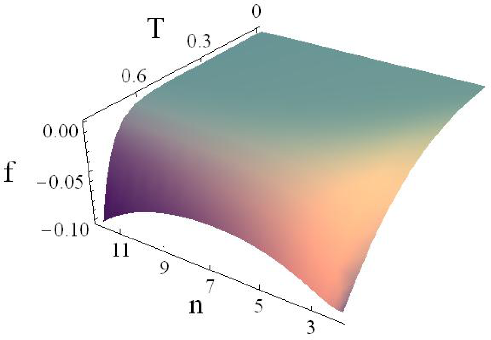
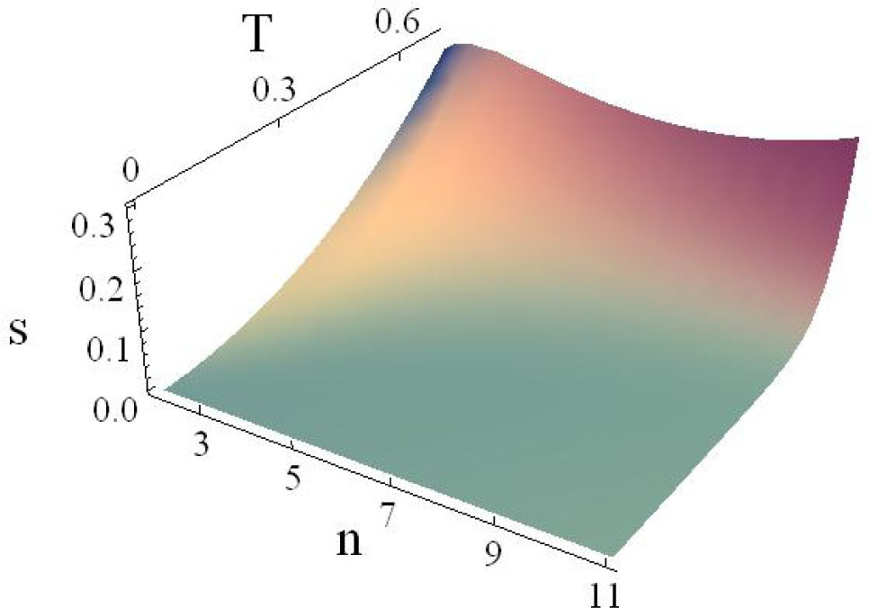
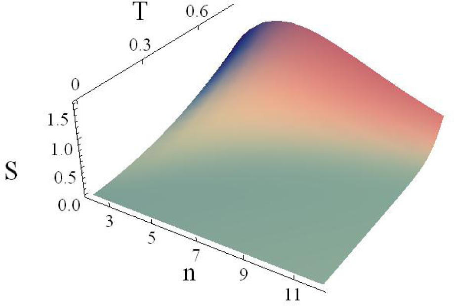
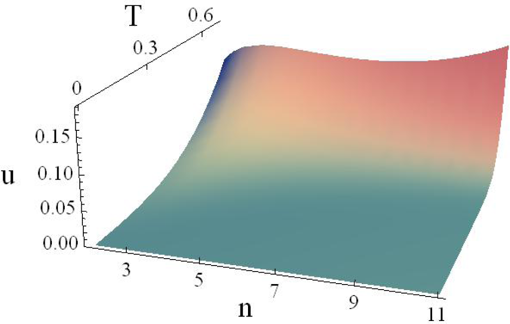
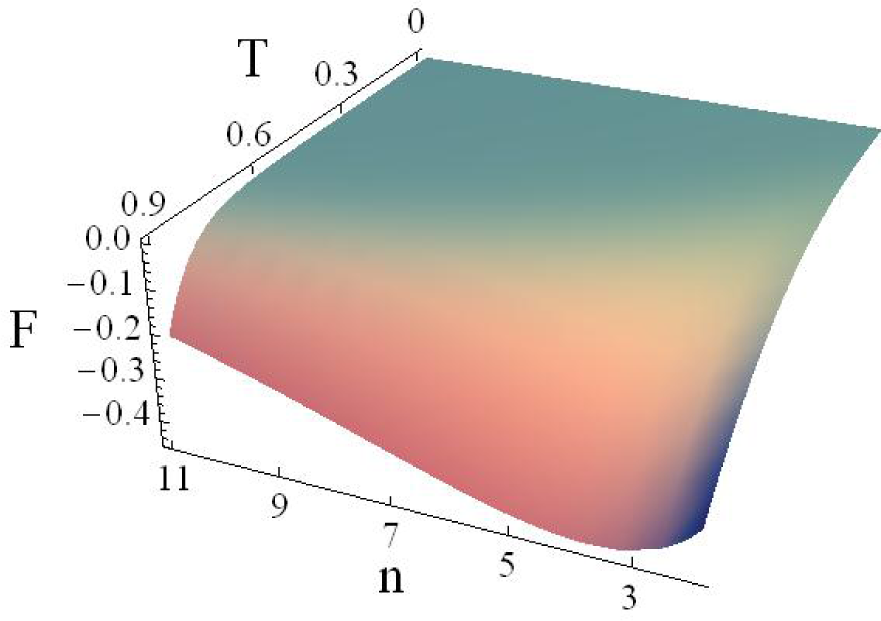
5. Critical Points of the Thermodynamic Potentials
Now, we shall analyze the behavior of energy, entropy and Helmholtz free energy densities (see
Figures 1 and
3). All of the potentials have a region of concavity or convexity along the
n-axis. Here,
n is just a parameter, and it is not a thermodynamic variable, since there is not a conjugate variable whose product has energy units and appears in the Gibbs equation. The units used are the so-called Planck or natural units [
41]. In this scale, the Planck temperature is
TP = 1.42 × 10
32K, and the energy of Planck is
EP = 1.9561 × 10
9J. In each plot, the most relevant region is the one at high temperatures and low dimensions, as can be seen in
Figures 1–
3.
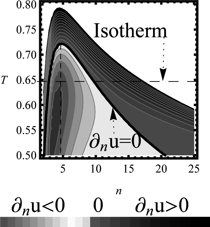
The functions
u (
n, T),
f (
n, T) and
s (
n, T) do not have a global maximum nor minimum, but for a given temperature, we can find both local maxima and minima for each potential along the
n-axis. These critical points are located in a certain range of
n and
T. Outside this region, the function presents a monotonic growth, because of the contribution of the term
ζ (
n + 1) Γ (
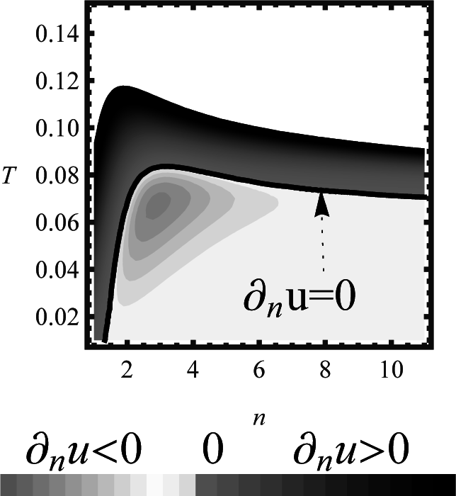
n + 1). One can analyze the first and second derivatives with respect to the dimension with the aim of determining whether the maxima and minima are restricted to a certain dimensionality. For example, at constant temperature, one can go from a minor to a major dimensionality, passing from positive to negative derivatives (or
vice versa) and the changes of sign of the derivatives are the maxima (or minima) of the energy density. As the temperature increases, the minima and maxima get closer to each other until they reach a saddle point (see
Figure 4).
One point is of special interest, the point at which one can no longer obtain any of both extreme points (nor minima nor maxima). The saddle point separates the regions of maxima and minima. This is summarized in
Table 1. Remarkably, the behavior of maxima, minima and saddle points (critical points) of
f,
s and
u along the
n-axis resembles the behavior of some first-order phase transitions in state equations of the van der Waals type, for example. For the case −
f =
p in the BBR system, the plane
p versus n is in general terms geometrically analogous to the plane
p versus V in the van der Waals case [
42]. However, evidently,
V is the conjugate thermodynamic variable of
p; meanwhile,
n does not have this property with respect to
p. We believe this analogy deserves to be deepened. In the case of the Helmholtz free energy, it would be of interest to determine if
n can take the role of the parameter of order in phase transitions. Furthermore, in stability analysis, the stability points are found where the critical points of
f,
u and
s are located.
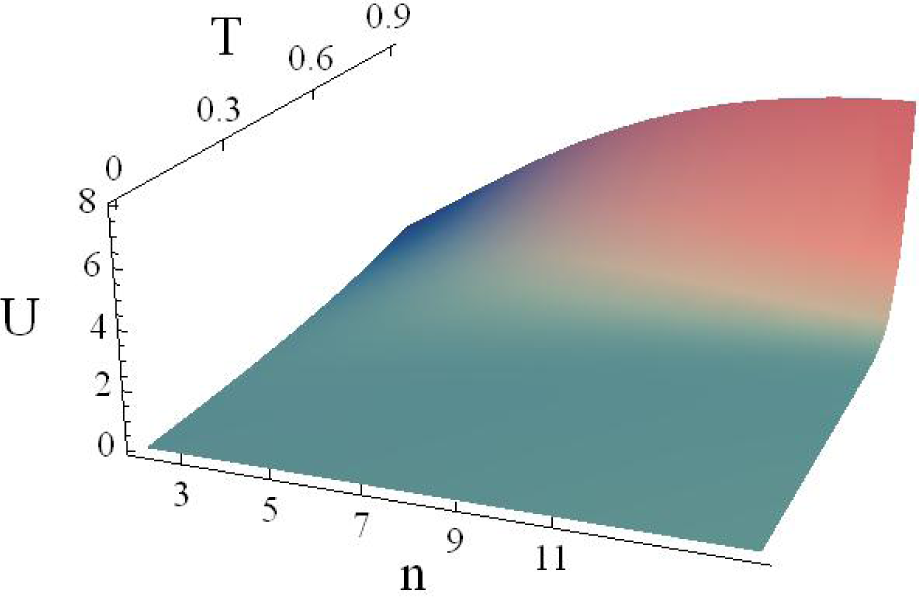
If a hypersphere is considered as the black body system, the total thermodynamic potential can be found. The volume of this hypersphere of radius
R is given by the expression [
35],
In
Figures 5–
7, the thermodynamic potentials
U (
n, T.R),
F (
n, T, R), and
S (
n, T, R) are shown (see
Equations (3),
(6) and
(7) respectively),
In these cases, we cannot find any restriction in the dimensionality at which the maxima or minima would appear. The variables R, T and n can be combined in several ways in order to produce critical points at any dimension.
6. A Possible Simple Application to Cosmology
Since the works by Kaluza and Klein [
7,
8], many proposals about the universe’s models with dimensionality different from three have been published [
7,
8,
18,
20,
22,
23,
32–
34,
43–
45]. Remarkably, this has been the case for papers stemming from string,
D−branes (where
D is for dimensionality) and gauge theories [
10–
14,
17,
22]. However, nowadays, we only have evidence for a universe with three space and one time dimensions. In the present section, we make a simple thermodynamic analysis leading to a scenario of a universe with only three space dimensions. This scenario is present within the region of high temperatures and low dimensionality mentioned in the previous section.
Temperatures as high as 10
32 K are only possible in a very primeval time in the evolution of the universe. It is known that the period dominated by radiation is from
t = 10
−44 s to
t ≈ 10
10 s [
46], that means that in this period, the universe could have been well described by a spatially-flat, radiation-only model [
47]. Thus, considering the whole primeval universe as a black body system in a Euclidean space is in principle a reasonable approach.
In some textbooks [
48,
49], the critical energy density at the time of
t ≈ 1
tP was about
u ≈ 1
EP/
VP (
VP is a Planck volume) and the temperature approximately
T ≈ 1
TP. The energy density and temperature obtained when the maximum of the energy density is located at
n = 3 (see
Figure 2) are surprisingly near the values referred to above.
For example, according to string theories, at some point (at the end of the Planck epoch), the rest of the dimensions remain small, and only the known three-dimensional space grew bigger. Another possibility is the mechanism known as dimensional reduction in the context of the Kaluza–Klein model [
50]. Although compact dimensions are not addressed in the context of this article, modifications to the integral with a cut-off frequency due to a finite size of the universe only introduce small corrections, as will be pointed out later. The remaining question is: why do we live in a 3-dimensional universe?
Let us suppose that by some sort of mechanism, the dimension of space was changed from a given initial value of the spatial dimensions to a final state with
n = 3. In this scenario, a change of energy can be obtained as is shown in
Table 2.
If such transitions would occur between an initial and a final dimension, a difference of energy could exist. In some cases, the “missing” energy represents a significant part of the total initial energy, as can be seen in
Table 3.
The energy difference between an initial and the final state is small for
n = 2 and
n = 4; for
n ≤ 10, the total energy is lower than the case
n = 3 for a Planck volume. In the cases
n = 9, 10, 25, the difference of energy may be relevant, and the questions of “where did that energy go?” and “could it be in some extra compactified dimensions?” may be relevant. In this model, we do not treat with compact dimensions, but this can be achieved by considering a maximum wave length in the integration of
Equation (2). For example, in a 9 + 1 space-time, the six extra spatial dimensions are supposed to be compactified, with a compactification related to the Planck scale [
32].
Table 3 means that a 3-dimensional universe should have been 0.89-times less energetic to form a two-dimensional space, 0.93-times less energetic for a four-dimensional space, 0.64-times less energetic for a 10-dimensional space and 11.5-times more energetic to form a 25-dimensional space. By increasing the temperature up to 1
TP, the difference between these energies is larger. For
T > 0.72
TP, the energy does not have any critical point, and the energy difference grows considerably for each initial dimensionality scenario.
Interestingly, the simple BBR system discussed here has a reasonable qualitative behavior relative to the universe’s entropy. It is believed that the early universe was in a state of incredibly low entropy [
51], and since then, the entropy has been growing according to the second law of thermodynamics. If we use the expression for the 3-dimensional BBR entropy (
S = 4
aVT3/3, with
a = 4
σ/
c) for calculating
S0 at the Planck scale and
Sf at the present time, immediately, one obtains
S0 ≈ 10
−23 J/K and
Sf ≈ 10
76 J/K, respectively. These values in Planck units are
S0 ≈ 1 and
Sf ≈ 10
99, which are within the range of other estimates [
51]. It should be noted that, in fact, if we consider the cosmological evolution of the universe, the entropy is conserved in the radiation-dominated era. However, the photons’ entropy grows due to the additional influence in the evolution of the universe, taking into account inflation, dark matter and dark energy components.
Notice that from
Equation (16) in an adiabatic expansion we have
T ∝ 1/
R, then, as the size of the universe decreases to zero (time is also tending to zero), the temperature increases to infinity, which may be related to an initial singularity.
If we want to include the evolution of the universe in our proposal, we could make the following suppositions. If we extrapolate the validity of the Einstein equations to just after the end of the Planck era, the corresponding fluid equation in an n-dimensional space reads:
For radiation
, and the dependence of the energy density
u in terms of the scale factor
a is
. The evolution of the the scale factor can be calculated from the Friedmann equation for a spatially-flat Universe:
where
κ could be related to the gravitational constant in
n-dim
Gn, (
κ =
4πn/2 Gn/
n(n − 2) Γ (
n/2); see [
52]) or to the Plank length in 3-dim
; see [
53]).
From the Friedmann equation, we get:
where
t0 = (4/
κU0(
n+1)
2)
1/2 is the present time, and the evolution of the energy density is described by:
Comparing the last equation with the Stefan–Boltzmann law in
n-dim, we obtain the dependence of the temperature of the radiation-dominated universe with time and the scale factor:
where:
However, there are several points that should be taken into account when the evolution of the universe is considered. The horizon distance is finite and could be calculated as follows:
This finite distance imposes an upper limit for the wavelength of photons inside the horizon and then a minimum frequency, and as a consequence, the dimensionless constants that describe the black body radiation should be changed, because they are calculated by means of integrals of the form:
where
. Considering that
λmax ∼
dh, the minimum
χ value is:
For example, for n = 3 and T = 0.9TP, the original integral should be reduced by a factor of order 10−3 when the value of χmin is considered. However, for T = 0.08TP, the two integrals are different by approximately 5%. For higher values of n, the difference between the integrals is even smaller.
In classical standard treatments, the energy density in a flat, radiation-only 3-dimensional universe is [
47]
with a horizon distance:
In an
n-dim Euclidean space with a volume
(sphere of radius
dhor), the total number of particles is then:
By using
Equations (17) and
(19), it is possible to find the following expression:
from
Equation (18) and considering the value
from [
53], then,
For
n = 3 and a temperature
T = 0.65
TP, the number of particles is
N ≈ 100; meanwhile, for
n = 9,
N ≈ 10
6. That is, in low dimensionality, the statistical behavior is not accurate. In fact, as
T →
TP, the number of photons tends to unity. The latter should be corrected if one pursues including the effects of the evolution of the universe near the Planck scale and the behavior of the black body radiation in the universe. The former issue is a very complicated problem, because the speed of light depends on the energy, and the quantum effects have to be incorporated by means of loop quantum cosmology, for example. One of the possible modifications consists of a different form of the dependence of the energy density on the scale factor,
ε =
ε0α(
a)
a−4 (see [
54]), where
α is calculated from loop quantum cosmology.
In the previous section, we saw that the maxima and minima are restricted to a certain dimensionality; thus, it could be a worthy effort to explore whether some thermodynamic property could intervene in the construction of a three-dimensional universe.
It is possible from this generalization of the Planck function to an Euclidean n-dimensional space to incorporate some corrections. Given the range of high temperatures, a modification of the dispersion relation found in LQG can be considered.
7. LQG Corrections
There is a large number of people in the scientific community that accept the possibility of the existence of extra dimensions besides the 3 + 1 known space-time dimensions. If one is willing to give the black body radiation a cosmological context, it is necessary to ask about the applicability of the above ideas in the regime of very high energies and temperatures. Nowadays, the necessity of having a theory that unifies the quantum world with general relativity in order to understand the possible scenarios of the high energy and the physics near the Planck epoch better is clear. One path to do this is by the modification of general relativity, that is quantum gravity, and this is the scope given by some important research programs. In the context of brane theories, it is possible to modify the geometrical part of the Einstein equations to incorporate extra dimensions, which have had certain success in explaining the dark energy problem and the interpretations of astronomical data [
31]. On the other hand, the extra dimensions are considered to have the size of the Planck scale and remain in a certain way hidden from our detectors [
10–
14,
17]. In a variety of quantum gravity treatments, string theory, LQG and doubly-special relativity, models based on non-commutative geometry, there exists a common topic: the dispersion relation modification. Some of these are related to addressing black hole thermodynamic problems. Nozari and Anvari in [
31] proposed a modification of the Planck law. This was made by using a modified dispersion relation showed in [
31,
55–
59], in which the square of the energy-momentum vector is:
where
LP is the Planck length and it depends on the dimensionality of the space-time [
57–
59],
E is the energy and
α and
α′ take different values depending on the details of the quantum gravity candidates. Finally, the spectral energy density in the interval
ν to
ν +
dν shown in [
31] is,
In this way, the internal energy density is given by the following expression (see [
31]),
and from
Equation (5) and
Appendix A, the Helmholtz free energy density now is,
One relevant aspect is that it is possible to get the same interesting behavior of the thermodynamic potential densities mentioned before, but one order of magnitude smaller in the temperature than in the model with no LQG modifications, as can be seen in
Figure 8 (see
Figure 4 for comparison). More importantly, the saddle point is located at
n ≈ 3.2. The location of the saddle point depends on the values of
α and
α′ of the quantum gravity candidates.
By using
Equation (7), we can calculate the entropy, which is the following,
and fulfills the relation
U =
F +
TS, that is
uV =
fV +
TsV. It is possible to obtain also the pressure, which is (according to
Equation (8))
p = −
f. The Gibbs potential is also zero, since
G =
F −
pV =
fV −
pV = 0.
Lets recall that this is a simple model, and the results obtained above should be considered as a qualitative behavior. It is remarkable that the behavior of the thermodynamic potentials is the same with and without LQG modifications. Notice that the maximum temperature at which there are no other critical points for the energy density
u is
T ≈ .08. In order to apply
Equation (24), the condition
E ≪ 1/
LP must be fulfilled. In this case, by dividing the total internal energy
U between the number of particles
N, it is possible to obtain a mean energy per photon
Emean, which is
Emean ≤ 0.3
EP. In the Taylor expansion (
Equation (24)), the terms of order higher than
are neglected, which corresponds to contributions on the order of 6.5 × 10
−5. In this way, the qualitative behavior of the model can be justified. In regards to the number of photons, when the classical cosmological approach is considered with no LQG modifications, the number of photons
N is
N ≈ 100 at
T = 0.65
TP, then statistical physics is not accurate. With the same classical cosmology approach and LQG modifications included, the number of photons at
T = .08 is such that
N > 5 × 10
5 for
n = 3 and
N > 10
34 for
n = 9. As mentioned before, this certainly must be corrected by quantum effects and a theory of quantum cosmology


