Article

Passive Decoy-State Quantum Key Distribution with Coherent Light

1
Escuela de Ingeniería de Telecomunicación, Department of Signal Theory and Communications, University of Vigo, Campus Universitario, Vigo 36310, Pontevedra, Spain
2
ICFO-Institut de Ciències Fotòniques, Mediterranean Technology Park, Castelldefels 08860, Barcelona, Spain
3
ICREA-Institució Catalana de Recerca i Estudis Avanc¸ats, Barcelona 08010, Spain
*
Author to whom correspondence should be addressed.
Entropy 2015, 17(6), 4064-4082; https://doi.org/10.3390/e17064064
Submission received: 31 March 2015 / Revised: 26 May 2015 / Accepted: 9 June 2015 / Published: 12 June 2015
(This article belongs to the Special Issue Quantum Cryptography)

Abstract

:
Signal state preparation in quantum key distribution schemes can be realized using either an active or a passive source. Passive sources might be valuable in some scenarios; for instance, in those experimental setups operating at high transmission rates, since no externally driven element is required. Typical passive transmitters involve parametric down-conversion. More recently, it has been shown that phase-randomized coherent pulses also allow passive generation of decoy states and Bennett–Brassard 1984 (BB84) polarization signals, though the combination of both setups in a single passive source is cumbersome. In this paper, we present a complete passive transmitter that prepares decoy-state BB84 signals using coherent light. Our method employs sum-frequency generation together with linear optical components and classical photodetectors. In the asymptotic limit of an infinite long experiment, the resulting secret key rate (per pulse) is comparable to the one delivered by an active decoy-state BB84 setup with an infinite number of decoy settings.

1. Introduction

Quantum key distribution (QKD) is already a mature technology that can provide cryptographic systems with an unprecedented level of security [1,2]. It aims at the distribution of a secret key between two distant parties (typically called Alice and Bob) despite the technological power of an eavesdropper (Eve) who interferes with the signals. This secret key is the essential ingredient of the one-time-pad or Vernam cipher [3], the only known encryption method that can offer information-theoretic secure communications.
Most practical long-distance implementations of QKD are based on the so-called Bennett–Brassard 1984 (BB84) protocol, introduced by Bennett and Brassard in 1984 [4], in combination with the decoy-state method [518]. In a typical quantum optical implementation of this scheme, Alice sends to Bob phase-randomized weak coherent pulses (WCPs) with different mean photon numbers that are selected, independently and randomly, for each signal. These states can be generated using a standard semiconductor laser together with a variable optical attenuator that is controlled by a random number generator (RNG) [1923]. Each light pulse may be prepared in a different polarization state, which is selected, again independently and randomly for each signal, between two mutually unbiased bases, e.g., either a linear (H [horizontal] or V [vertical]) or a circular (L [left] or R [right]) polarizations basis. For simplicity, we will first consider the case of polarization encoding. Later in this paper, we will also examine phase encoding. For that, two main experimental configurations are typically used. In the first one, Alice employs four laser diodes, one for each possible BB84 signal [24,25]. These lasers are controlled by a RNG that decides each given time which one of the four diodes is triggered. The second configuration utilizes only one laser diode in combination with a polarization modulator [2630]. This modulator rotates the state of polarization of the signals depending on the output of a RNG. On the receiving side, Bob measures each incoming signal by choosing at random between two polarization analyzers, one for each possible basis. Once the quantum communication phase of the protocol is completed, Alice and Bob use an authenticated public channel to process their data and obtain a secure secret key. Importantly, the security of decoy-state QKD has been obtained both in the asymptotic regime [6,7] and in the case of finite-length keys [31,32].
Alternatively to the active signal state preparation methods described above, Alice may as well employ a passive transmitter to generate decoy-state BB84 signals. This last solution might be desirable in some scenarios; for instance, in those experimental setups operating at high transmission rates, since no RNGs are required in a passive device [3341]. Passive schemes might also be more robust against certain side-channel attacks hidden in the imperfections of some optical components like, for example, optical modulators used in the active sources. If a polarization modulator (or an amplitude or phase modulator) is not properly designed, for example, it may distort some of the physical parameters of the pulses emitted by the sender depending on the particular value of the polarization setting selected. This fact could open a security loophole in the active schemes.
The working principle of a passive transmitter is rather simple. For example, Alice can use various light sources to produce different signal states that are sent through an optics network. Depending on the particular detection pattern observed in some properly located photodetectors, she can infer which signal states are actually generated. Known passive schemes rely typically on the use of a parametric down-conversion (PDC) source, where Alice and Bob passively and randomly choose which bases to measure each incoming pulse by means of a beamsplitter (BS) [40,41]. Also, Alice can exploit the photon number correlations that exist between the two output modes of a PDC source to passively generate decoy states [34]. More recently, it has been shown that phase-randomized coherent pulses are also suitable for passive preparation of decoy states [37,38] and BB84 polarization signals [42], though the combination of both setups in a single passive source is cumbersome. Intuitively speaking, Refs. [37,38,42] take advantage of the random phase of the different generated pulses to passively prepare states with either distinct photon number statistics but with the same polarization [37,38], or with different polarizations but equal intensities [42]. The preparation of phase-randomized coherent pulses could be achieved, for instance, by strongly modulating the laser diode, taking it below and above threshold [21,22].
In this article, we present a complete passive decoy-state QKD transmitter with coherent light. It shows that it is indeed possible to do state preparation for QKD in an entirely passive way using coherent states, even for BB84 signals in combination with decoy levels. Our method employs sum-frequency generation (SFG) [4346] together with linear optical components and classical photodetectors. SFG has already exhibited its usefulness in quantum information [4752] and device-independent QKD [53] at the single-photon level. Here we use it in the conventional non-linear optics paradigm with strong coherent light. This fact might render our proposal particularly valuable from an experimental point of view. In the asymptotic limit of an infinite long experiment, it turns out that the secret key rate (per pulse) provided by such passive scheme is similar to the one delivered by an active decoy-state BB84 setup with infinite decoy settings. Let us emphasize, however, that it is uncertain whether in practice such passive scheme could beat active transmitters or passive solutions based on a PDC source in high-speed QKD in general. Importantly, the answer will depend on various technologies.
The paper is organized as follows. In Section 2 we introduce a passive transmitter that generates decoy-state BB84 polarization signals using coherent light. Then, in Section 3 we evaluate its performance and we obtain a lower bound on the resulting secret key rate in the asymptotic regime. In Section 4 we consider the case where Alice and Bob use phase-encoding, which is more suitable to employ in combination with optical fibers than polarization encoding. Finally, Section 5 concludes the article with a summary. The paper includes as well some Appendixes with additional calculations.

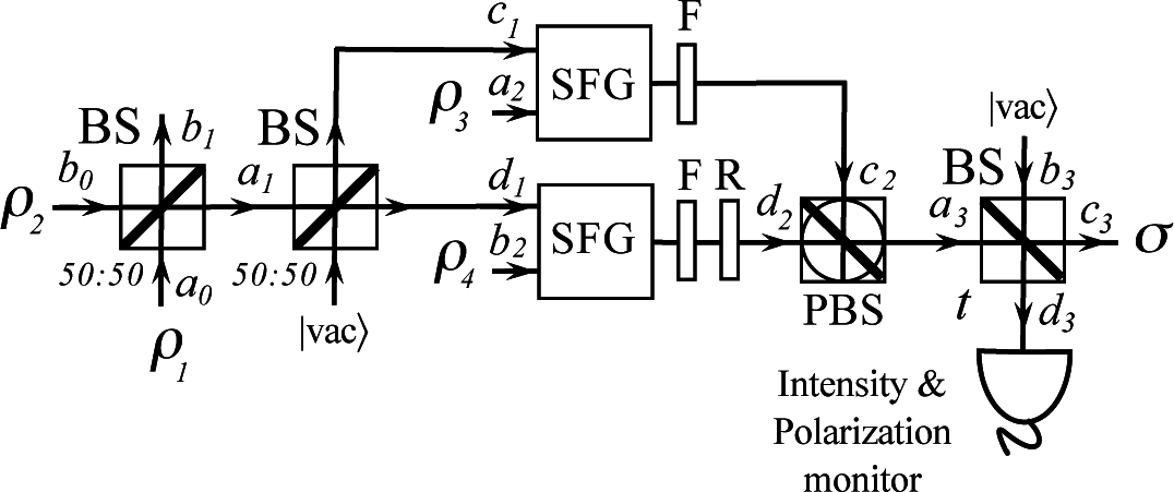
2. Passive Decoy-State BB84 Transmitter

The basic setup is illustrated in Figure 1.
Let us start considering, for simplicity, the interference of two pure coherent states of frequency w1, both prepared in +45° linear polarization and with arbitrary phase relationship, | 2 μ e i θ 1 a 0 , + 45 ° and | 2 μ e i θ 2 b 0 , + 45 °, at a 50 : 50 BS. The output states in modes a1 and b1 (see Figure 1) are given by
| μ ( e i θ 1 + e i θ 2 ) a 1 , + 45 ° | μ ( e i θ 1 e i θ 2 ) b 1 , + 45 ° .
Then, we have that the output states in modes c1 and d1 have the form
| μ 2 ( e i θ 1 + e i θ 2 ) c 1 , + 45 ° | μ 2 ( e i θ 1 e i θ 2 ) d 1 , + 45 ° .
If these two states are combined with two coherent states of frequency w2, | μ e i θ 3 a 2 , + 45 ° and | μ e i θ 4 b 2 , + 45 °, in a nonlinear medium using the SFG process, the resulting output states at frequency w3 = w1 + w2, after the polarization rotation R, can be written as (see Appendix A)
| μ e i θ 3 ( e i θ 1 + e i θ 2 ) 2 c 2 , + 45 ° | μ e i θ 4 ( e i θ 1 + e i θ 2 ) 2 d 2 , 45 ° .
These two beams are now re-combined at a PBS in the ±45° linear polarization basis [54]. We obtain that the output state in mode a3 (see Figure 1) is a coherent state of the form
| ζ ( θ ) e i ϕ ψ , a 3 = e ζ ( θ ) / 2 n = 0 ( ζ ( θ ) e i ϕ ) n n ! | n ψ ,
where ζ(θ) = 2µ(1 + cos θ), θ = θ2 − θ1, ϕ = π + θ1 + θ3 + arg (1 + e), and the Fock states |nψ〉 are given by
| n ψ = [ 1 2 ( a + 45 ° + e i ψ a 45 ° ) ] n n ! | vac ,
with |vac〉 denoting the vacuum state and ψ = θ4 − θ3. Finally, Alice sends the quantum state given by Equation (4) through a BS of transmittance t ≪ 1. Then, the output states in modes c3 and d3 are given by
| t ζ ( θ ) e i ϕ ψ , c 3 | ( 1 t ) ζ ( θ ) e i ϕ ψ , d 3 .
The analysis of the case where the global phase of each input signal ρi, with i ∈ {1,…, 4}, is randomized and inaccessible to the eavesdropper is now straightforward. It can be solved by just integrating the signals | t ζ ( θ ) e i ϕ ψ , c 3 and | ( 1 t ) ζ ( θ ) e i ϕ ψ , d 3 given by Equation (6) over all angles θ, ϕ, and ψ. In particular, we have that the output state σ in this scenario (see Figure 1) can be written as
σ = 1 ( 2 π ) 3 ϕ , θ , ψ | t ζ ( θ ) e i ϕ ψ , c 3 t ζ ( θ ) e i ϕ | d ϕ d θ d ψ = 1 ( 2 π ) 2 θ e γ ( θ ) n = 0 γ ( θ ) n n ! ψ | n ψ n ψ | d θ d ψ ,
where the intensity γ(θ) is given by γ(θ) = (θ). As already mentioned previously, note that the generation of phase-randomized coherent states can be achieved, for example, by using strong current modulation of the laser diode, well above and below threshold, which ensures a true random phase (unknown to the eavesdropper) for each prepared pulse [21,22].
The weak intensity signal σ in mode c3 is suitable for QKD and Alice sends it to Bob through the quantum channel. In addition, she uses the strong intensity signal available in mode d3 to measure both its intensity and polarization. This last measurement can be realized, for example, by means of a passive BB84 detection scheme where the basis choice is performed by a 50 : 50 BS, and on each end there is a PBS and two classical photodetectors. From the different intensities observed in each of these four photodetectors, Alice can determine both the value of the angle ψ and the total intensity of the signal. Note that, by assumption, we have that the intensity of the input states ρi is very high.
Intuitively speaking, the working principle of the setup illustrated in Figure 1 is quite simple. In a first step, the setup passively generates in mode a1 coherent states of random amplitude. This is done by combining two coherent states or equal amplitude but random phase at a BS. This part follows the approach proposed in [37,38] to passively prepare decoy states. Then, in a second step, the setup generates signals whose photons are randomly polarized within the X-Z plane of the Bloch sphere. For this, it first prepares two phase-randomized coherent states of the same amplitude in +45° and −45° linear polarization, and then interferes them at a PBS. This approach is inspired by the solution introduced in [42]. Indeed, this is the role of the interferometric part of the scheme, where the SFG process is actually used to imprint a random phase to each state. Finally, in a third step, the setup attenuates the generated signals to the single-photon level before they are sent to Bob, and it also determines both the intensity and polarization of the signals prepared.
For simplicity, let us assume for the moment that the polarization measurement is perfect, i.e., for each incoming signal it provides Alice with a precise value for the measured angle ψ, while the intensity measurement only tells her whether the measured intensity is below or above a certain threshold value Λ that satisfies 0 < Λ < 4µ(1 − t). That is, Λ is between the minimal and maximal possible values of the intensity (1 − t)ζ(θ) of the optical pulses in mode d3. The first intensity interval, ξd = [0, Λ], can be associated, for instance, to the generation of a decoy state in output mode c3 (that we shall denote as σd), while the second intensity interval, ξs = [Λ, 4µ(1−t)], corresponds to the case of preparing a signal state (σs). Note, however, that the analysis presented in this section can be straightforwardly adapted to cover as well the case of several intensity intervals ξi (i.e., the generation of several decoy states). Figure 2 (case A) shows a graphical representation of the intensity (1 − t)ζ(θ) in mode d3 versus the angle θ, together with the threshold value Λ and the intensity intervals ξd and ξs.
The threshold angle θΛ that satisfies (1 − t)ζ(θΛ) = Λ is given by
θ Λ = arccos ( Λ 2 μ ( 1 t ) 1 ) .
In this simplified scenario, the conditional quantum states that are sent to Bob can be written as
σ i , ψ = n = 0 p n i | n ψ n ψ | ,
where i = {s, d}, and the probabilities p n i are given by
p n s = 1 θ Λ 0 θ Λ e γ ( θ ) γ ( θ ) n n ! d θ , p n d = 1 π θ Λ θ Λ π e γ ( θ ) γ ( θ ) n n ! d θ .
In practice, however, it is not necessary that Alice determines the value of ψ accurately and restricts herself to only those events where she actually prepares a perfect BB84 polarization state (i.e., when the angle ψ satisfies ψ ∈ {0, π/2, π, 3π/2}) [42]. Note that the probability associated with these ideal events tends to zero. Instead, it is sufficient if the polarization measurement tells her the value of ψ within a certain interval around the desired ideal values. This situation is illustrated in Figure 2 (case B), where Alice selects some valid regions (marked with gray color in the figure) for the angle ψ [42]. These regions depend on an acceptance parameter Ω ∈ [0, π/4] that we optimize. In particular, whenever the value of ψ lies within any of the valid regions, Alice considers the pulse emitted by the source as a valid signal. Otherwise, the pulse is discarded afterwards during the post-processing phase of the protocol, and it does not contribute to the key rate. The probability that a pulse is accepted, pacc, is given by
p acc = 1 4 Ω π .
There is a trade-off on the acceptance parameter Ω. A high acceptance probability pacc favors Ω 0, but this action also results in an increase of the quantum bit error rate (QBER) of the protocol. A low QBER favors Ω ≈ π/4, but then pacc 0. Note that in the limit where Ω tends to π/4 we recover the standard decoy-state BB84 protocol.

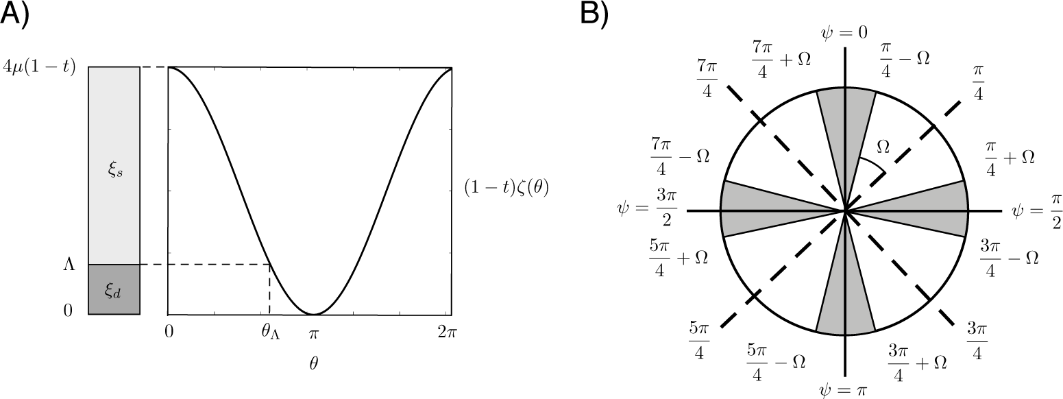
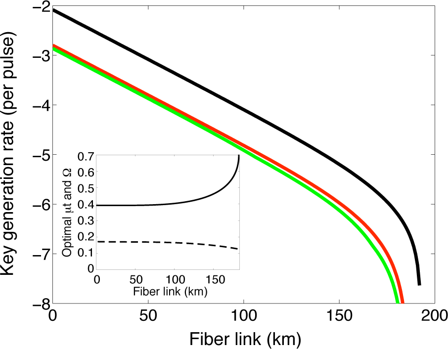
3. Lower Bound on the Secret Key Rate
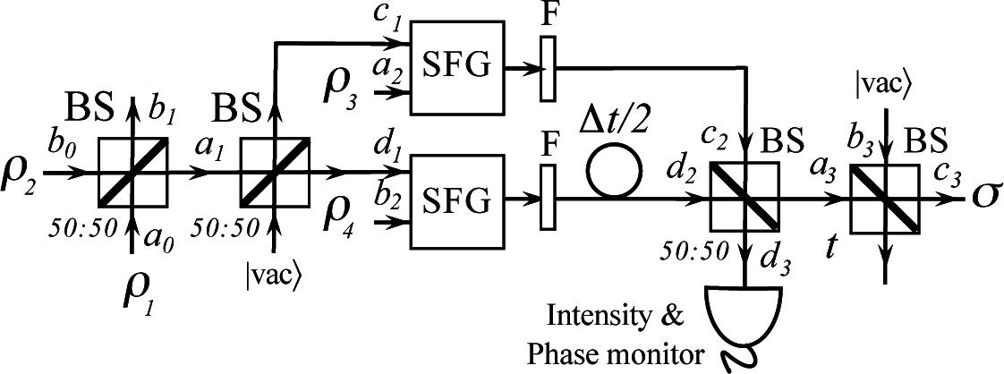
We shall consider that Alice and Bob treat decoy and signal states separately, and they distill secret key from both of them. For that, we use the security analysis presented in [6], which combines the results provided by Gottesman–Lo–Lütkenhaus–Preskill (GLLP) in [55] (see also [56]) with the decoy-state method. It can be shown that the single-photon signals emitted by the passive source illustrated in Figure 1, averaged over the values of Alice’s key bit, are basis-independent [42]. This analysis is valid for the asymptotic regime of infinitely long keys. The secret key rate formula can be written as
R i p i max { R i , 0 } ,
with i = {s, d}. Here pi denotes the probability to generate a state associated to the intensity interval ξi (i.e., ps = θΛ and pd = 1 − ps), and
R i q p acc { Q i f ( E i ) H ( E i ) + p 1 i Y 1 [ 1 H ( e 1 ) ] + p 0 i Y 0 } .
The parameter q is the efficiency of the protocol (q = 1/2 for the standard BB84 scheme, and q ≈ 1 for its efficient version [57]); Qi denotes the gain, i.e., the probability that Bob obtains a click in his measurement apparatus when Alice sends him a signal σi; f(Ei) represents the efficiency of the error correction protocol as a function of the error rate Ei, typically f(Ei) ≥ 1 with Shannon limit f(Ei) = 1 [58]; Yn is the yield of an n-photon signal, i.e., the conditional probability of a detection event on Bob’s side given that Alice transmits an n-photon state; en denotes the error rate of an n-photon signal; and H(x) = −x log2 (x) (1 − x) log2 (1 − x) represents the binary Shannon entropy function.
For simulation purposes, we shall consider a simple channel model in the absence of eavesdropping [6,59]; it consists of a BS whose transmittance depends on the transmission distance and on the loss coefficient of the quantum channel. That is, for simplicity, we neglect any misalignment effect in the channel. Furthermore, we assume that Bob employs an active BB84 detection setup. This model allows us to calculate the observed experimental parameters Qi and Ei. These quantities are given in Appendix B. Our results, however, can also be straightforwardly applied to any other channel model or detection setup, as they depend only on the observed gain and QBER.
To evaluate the secret key rate formula given by Equation (13) we need to estimate the yields Y0 and Y1, together with the single-photon error rate e1, by solving the following set of linear equations:
Q i = n = 0 p n i Y n , and Q i E i = n = 0 p n i Y n e n .
For that, we shall use the procedure proposed in [38,59]. Moreover, we will assume a random background (i.e., e0 = 1/2).
This method requires that the probabilities p n i given by Equation (10) satisfy certain conditions that we confirm numerically. The results are included in Appendix C. It is important to emphasize, however, that the estimation technique presented in [38,59] only constitutes a possible example of a finite decoy-state setting estimation procedure. In principle, many other estimation methods are also available for this purpose, such as linear programming tools [60], which might result in sharper, or for the purpose of QKD, better bounds on the considered probabilities.
The resulting lower bound on the secret key rate with two intensity settings is illustrated in Figure 3 (green line). In our simulation we employ the following experimental parameters: the dark count rate of Bob’s detectors is ϵB = 3.2×10⁻⁷, the overall transmittance of Bob’s detection apparatus is ηB = 0.045, and the loss coefficient of the channel is α = 0.2 dB/km. We further assume that q = 1/2, and f(Ei) = 1.22. With this configuration, it turns out that the optimal value of the parameter µt decreases with increasing distance, while the optimal value of the parameter Ω increases with the distance. A similar behavior was also observed in the passive BB84 transmitter (without decoy states) proposed in [42]. In particular, µt diminishes from 0.175 to 0.125, while Ω augments from 0.393 to 0.7. At long distances the gain of the protocol is very low and, therefore, it is important to keep both the multi-photon probability of the source (related with the parameter µt) and the intrinsic error rate of the signals sent by Alice (related with the parameter Ω) also low. Figure 3 includes as well an inset plot with the optimized parameters µt (dashed line) and Ω (solid line). The optimal value for the parameter Λ turns out to be constant with the distance; it is given by Λ = 2µ(1 − t), i.e., the threshold angle θΛ is equal to π/2. This figure also shows a lower bound on the secret key rate for the cases of an active decoy-state BB84 system with infinite decoy settings (black line) [6], and a passive transmitter with infinite intensity intervals ξi (red line). The cutoff points where the secret key rate drops down to zero are 181 km (passive setup with two intensity settings), 183 km (passive setup with infinite intensity settings), and 192 km (active transmitter with infinite decoy settings). From the results shown in Figure 3 we see that the performance of the passive transmitter presented in Section 2, with only two intensity settings, is similar to that of an active asymptotic setup, thus showing the practical interest of the passive scheme. The relatively small difference between the achievable secret key rates in both scenarios is due to two main factors: (a) the intrinsic error rate of the signals accepted by Alice, which is zero only in the case of an active source; and (b) the probability pacc to accept a pulse emitted by the source, which is pacc < 1 in the passive setup and pacc = 1 in the active scheme. For instance, we have that for most distances Ω 0.393, which implies pacc 0.5. This fact reduces the key rate on logarithmic scale of the passive transmitter by a factor of log10 pacc 0.3. The additional factor of 0.45 that can be observed in Figure 3 arises mainly from the intrinsic error rate of the signals.

4. Phase Encoding

Similar ideas to the ones presented in Section 2 can also be used in other implementations of the decoy-state BB84 protocol with a different signal encoding. For instance, in those QKD experiments based on phase encoding, which is more suitable to use with optical fibers than polarization encoding, which is particularly relevant in the context of free-space QKD [1,2].
The basic setup is illustrated in Figure 4.
Again, for simplicity, let us consider first the case where the input signals ρi, with i ∈ {1,…, 4}, are pure coherent states with arbitrary phase relationship: | 2 μ e i θ 1 a 0 , + 45 ° and | 2 μ e i θ 2 b 0 , + 45 ° (of frequency w1), and | μ e i θ 3 a 2 , + 45 ° and | μ e i θ 4 b 2 , + 45 ° (of frequency w2). Let Δt denote the time difference between two consecutive pulses generated by the sources. Then, from Section 2 we have that the signals in modes c2 and d2 at time instances t and t + Δt/2 can be written as
| ζ ( θ ) 2 e i ϕ t c 2 , + 45 ° | ζ ( θ ) 2 e i ϕ t + Δ t / 2 d 2 , + 45 ° ,
where ϕ= ϕ + θ4 − θ3. Similarly, we find that the quantum states in modes c3 and d3 are given by, respectively,
| γ ( θ ) 2 e i ϕ t c 3 , + 45 ° | γ ( θ ) 2 e i ϕ t + Δ t / 2 c 3 , + 45 ° , | ζ ( θ ) 2 e i ϕ t d 3 , + 45 ° | ζ ( θ ) 2 e i ϕ t + Δ t / 2 d 3 , + 45 ° .
The case of phase-randomized strong coherent pulses is completely analogous to that of Section 2 and we omit it here for simplicity; it results in an uniform distribution for the angles θ, ϕ, and ϕ′ for both pairs of pulses given by Equation (16). The strong signals in mode d3 are used to measure both their phases, relative to some local reference phase, and their intensities by means of an intensity and phase measurement, while Alice sends the weak signals in mode c3 to Bob. Again, just like in the passive source with polarization encoding shown in Figure 1, Alice can now select some valid regions for the measured phases and also distinguish between different intensity settings. Then, we have that the analysis and results presented in Section 3 also apply straightforwardly to this scenario.

5. Conclusions

In this paper, we have introduced a complete passive transmitter for QKD that can prepare decoy-state Bennett-Brassard 1984 signal states using coherent light. Our method employs sum-frequency generation together with linear optical components and classical photodetectors. In the asymptotic limit of an infinite long experiment, we have proven that such passive scheme can provide a secret key rate (per pulse) lower but comparable to the one delivered by an active decoy-state BB84 setup with infinite decoy settings. In practice, however, it is uncertain if the passive scheme will be able to beat active transmitters or passive solutions based on PDC sources in general; the answer will depend on various technologies [63,64].
The main focus of this paper has been polarization-based realizations of the BB84 protocol, which are particularly relevant for free-space QKD. However, we have also shown that similar ideas can as well be applied to other practical scenarios with different signal encodings, like, for instance, those QKD experiments based on phase encoding, which are more suitable for use in combination with optical fibers.

Acknowledgments

We thank F. Steinlechner for helpful discussions. This work was supported by the Galician Regional Government (program “Ayudas para proyectos de investigación desarrollados por investigadores emergentes”, and consolidation of Research Units: AtlantTIC), the Spanish Ministry of Economy and Competitiveness (MINECO) project MAGO (Ref. FIS2011-23520), the “Fondo Europeo de Desarrollo Regional” (FEDER) through grants TEC2013-46168-R and TEC2014-54898-R, and the European Research Council project AQUMET.

Appendix

A. Sum-Frequency Generation

For completeness, in this Appendix we include the calculations to derive Equation (3) in Section 2. Our starting point are the input states to one of the two SFG processes used in the passive transmitter illustrated in Figure 1: | μ 2 ( e i θ 1 + e i θ 2 ) c 1 , + 45 ° and | μ e i θ 3 a 2 , + 45 °. Such process is described by the Hamiltonian H = i χ ( c 1 a 2 c 2 H . c . ), where c 2 represents the creation operator for the light wave at frequency w3 = w1 + w2 [45]. The parameter χ is a coupling constant that is proportional to the second-order susceptibility χ(2) of the nonlinear material, and H.c. denotes a Hermitian conjugate. When the pump mode at frequency w2 is kept strong and undepleted, then this mode can be typically treated classically as a complex number. With this assumption, we have that the effective Hamiltonian above can now be written as H = i χ ( μ e i θ 3 c 1 c 2 H . c . ). Using the Heisenberg equation of motion, it is straightforward to obtain the following coupled-mode equations:
d c 1 d t = χ μ e i θ 3 c 2 , d c 2 d t = χ μ e i θ 3 c 1 ,
which can be solved in terms of initial values at t = 0 to yield
c 1 ( t ) = c 1 ( 0 ) cos ( μ χ t ) e i θ 3 c 2 ( 0 ) sin ( μ χ t ) c 2 ( t ) = c 2 ( 0 ) cos ( μ χ t ) + e i θ 3 c 1 ( 0 ) sin ( μ χ t ) .
At the point of complete conversion, t c = π / ( 2 μ χ ), we obtain
c 1 ( t c ) = e i θ 3 c 2 ( 0 ) , c 2 ( t c ) = e i θ 3 c 1 ( 0 ) .
That is, at time tc we find that the resulting output state at frequency w3 from the SFG process is given by
| μ 2 e i θ 3 ( e i θ 1 + e i θ 2 ) c 2 , + 45 ° .

B. Gain and QBER

In this Appendix, we obtain a mathematical expression for the observed gains Qi and error rates Ei, with i ∈ {s, d}, for the passive QKD transmitter with two intensity settings introduced in Section 2. For that, we employ the typical channel model in the absence of eavesdropping [6,59]; it just consists of a BS of transmittance η channel = 10 α d 10, where α denotes the loss coefficient of the channel measured in dB/km and d is the transmission distance. Moreover, for simplicity, we consider that Bob employs an active BB84 detection setup with two threshold detectors.
The action of Bob’s measurement device can be described by two positive operator value measures (POVMs), one for each of the two BB84 polarization bases β ∈ {l, c}, with l denoting a linear polarization basis and c a circular polarization basis. Each POVM contains four elements: G VAC β, G 0 β, G 1 β, and G dc β. The first one corresponds to the case of no click in the detectors, the following two POVM operators give precisely one detection click, and the last one, G dc β, gives rise to both detectors being triggered. These operators can be written as [42]
G VAC β = [ 1 ϵ B ( 2 ϵ B ) ] F VAC β , G 0 β = ( 1 ϵ B ) ϵ B F VAC β + ( 1 ϵ B ) F 0 β , G 1 β = ( 1 ϵ B ) ϵ B F VAC β + ( 1 ϵ B ) F 1 β , G dc β = I G VAC β G 0 β G 1 β .
Here we assume that the background rate is, to a good approximation, independent of the signal detection. Moreover, for easiness of notation, we consider only a background contribution coming from the dark count rate ϵB of Bob’s detectors and we neglect other background contributions like, for instance, stray light arising from timing pulses which are not completely filtered out in reception. The operators F VAC β, F 0 β, F 1 β, and F dc β have the form
F VAC β = n , m = 0 ( 1 η sys ) n + m | n , m β n , m | , F 0 β = n , m = 0 [ 1 ( 1 η sys ) n ] ( 1 η sys ) m | n , m β n , m | , F 1 β = n , m = 0 [ 1 ( 1 η sys ) m ] ( 1 η sys ) n | n , m β n , m | , F dc β = n , m = 0 [ 1 ( 1 η sys ) n ] [ 1 ( 1 η sys ) m ] × | n , m β n , m | ,
with β ∈ {l, c}. The signals |n, ml (|n, mc) represent the state which has n photons in the horizontal (circular left) polarization mode and m photons in the vertical (circular right) polarization mode. The parameter ηsys denotes the overall transmittance of the system. This quantity can be written as ηsys = ηBηchannel, where ηB is the overall transmittance of Bob’s detection apparatus, i.e., it includes the transmittance of any optical component within Bob’s measurement device together with the efficiency of his detectors.
In the scenario considered, it turns out that the gains Qi are independent of the actual polarization of the signals σi,ψ given by Equation (9) and the basis β used to measure them. We obtain
Q i = 1 Tr ( G vac β σ i , ψ ) = 1 ( 1 ϵ B ) 2 p i π θ ξ i e η sys γ ( θ ) d θ ,
where ps = θΛ, pd = 1 − ps, θ ξ s = [ 0 , θ Λ ], and θ ξ d = [ θ Λ , π ].
When θΛ = π/2, which is the value that maximizes the secret key rate formula given by Equation (12), we have that the gains Qi can be written as
Q s = 1 ( 1 ϵ B ) 2 A ( η sys ζ ) , Q d = 1 ( 1 ϵ B ) 2 A + ( η sys ζ ) ,
where ζ = 2µt, and
A ± ( x ) = e x [ I 0 , x ± L 0 , x ] .
Here Iq,z represents the modified Bessel function of the first kind, and Lq,z denotes the modified Struve function. These functions are defined as [61,62]
I q , z = 1 2 π i e ( z / 2 ) ( t + 1 / t ) t q 1 d t , L q , z = z q 2 q 1 π Γ q + 1 / 2 0 π / 2 sinh ( z cos θ ) sin θ 2 q d θ .
The error rates Ei depend on the value of the angle ψ. By symmetry, we can restrict ourselves to evaluate the QBER in only one of the valid regions for ψ. Note that is the same in all of them. For instance, let us consider the case where ψ ∈ [7π/4 + Ω, π/4 Ω] (which corresponds to the horizontal polarization interval), and let E ψ i denote the error rate of a signal σi,ψ in that region. This quantity can be written as
E ψ i = 1 Q i Tr [ ( G 1 l + 1 2 G dc l ) σ i , ψ ] .
Here we have considered the typical initial post-processing step in the BB84 protocol, where double-click events are not discarded by Bob, but are randomly assigned to single-click events. Equation (27) can be further simplified as
E ψ i = 1 2 Q i { ϵ B ( ϵ B 1 ) f 0 , ψ i + [ 2 + ϵ B ( ϵ B 3 ) ] f 1 , ψ i + ( 1 ϵ B ) 2 f dc, ψ i + ϵ B ( 2 ϵ B ) } ,
where f j , ψ i = Tr ( F j l σ i , ψ i ). After a short calculation, we obtain
f 0 , ψ i = 1 p i π θ ξ i e η sys γ ( θ ) [ 1 + e 1 2 η sys γ ( θ ) ( 1 + cos ψ ) ] d θ , f 1 , ψ i = 1 p i π θ ξ i e η sys γ ( θ ) [ 1 + e 1 2 η sys γ ( θ ) ( 1 + cos ψ ) ] d θ , f dc , ψ i = 1 + 1 p i π θ ξ i e η sys γ ( θ ) e 1 2 η sys γ ( θ ) ( 1 cos ψ ) e 1 2 η sys γ ( θ ) ( 1 + cos ψ ) d θ .
when θΛ = π/2, these expressions can be simplified as
f 0 , ψ s = A ( η sys ζ ) + A [ κ + ( ψ ) ] , f 0 , ψ d = A + ( η sys ζ ) + A + [ κ + ( ψ ) ] , f 1 , ψ s = A ( η sys ζ ) + A [ κ ( ψ ) ] , f 1 , ψ d = A + ( η sys ζ ) + A + [ κ ( ψ ) ] , f dc , ψ s = 1 + A ( η sys ζ ) A [ ϵ + ( ψ ) ] A [ ϵ ( ψ ) ] , f dc , ψ d = 1 + A + ( η sys ζ ) A + [ ϵ + ( ψ ) ] A + [ ϵ ( ψ ) ] ,
where the parameters κ±(ψ) and ϵ±(ψ) have the form
κ ± ( ψ ) = η sys ζ [ 1 ( 1 ± cos ψ ) / 2 ] , ϵ ± ( ψ ) = η sys ζ ( 1 ± cos ψ ) / 2.
The quantum bit error rates Ei are then given by
E i = 2 π 4 Ω 7 π 4 + Ω π 4 Ω E ψ i d ψ .
Combining Equations (28) and (30)–(32), we find that
E s = 1 2 Q s { 1 ( 1 ϵ B ) 2 A ( η sys ζ ) + 2 π 4 Ω 7 π 4 + Ω π 4 Ω ϵ B ( ϵ B 1 ) A [ κ + ( ψ ) ] + [ 2 + ϵ B ( ϵ B 3 ) ] A [ κ ( ψ ) ] ( 1 ϵ B ) 2 [ A [ ϵ + ( ψ ) ] + A [ ϵ ( ψ ) ] ] d ψ } ,
and
E d = 1 2 Q d { 1 ( 1 ϵ B ) 2 A + ( η sys ζ ) + 2 π 4 Ω 7 π 4 + Ω π 4 Ω ϵ B ( ϵ B 1 ) A + [ κ + ( ψ ) ] + [ 2 + ϵ B ( ϵ B 3 ) ] A + [ κ ( ψ ) ] ( 1 ϵ B ) 2 [ A + [ ϵ + ( ψ ) ] + A + [ ϵ ( ψ ) ] ] d ψ } ,
and we solve these equations numerically.

C. Estimation procedure

The secret key rate formula given by Equation (13) can be lower bounded by
R i q p acc { Q i f ( E i ) H ( E i ) + ( p 1 i Y 1 + p 0 i Y 0 ) [ 1 H ( e 1 U ) ] } ,
where e 1 U denotes an upper bound on the single-photon error rate e1. Hence, for our purposes, it is enough to obtain a lower bound on the quantities p 1 i Y 1 + p 0 i Y 0 for all i ∈ {s, d}, together with e 1 U. For that, we can directly use the results obtained in [38], which we include in this Appendix for completeness. The probabilities p n i given by Equation (10) need to satisfy certain conditions that we confirm numerically. In particular, we have that
p 1 i Y 1 + p 0 i Y 0 max { p 1 i ( p 2 d Q s p 2 s Q d ) p 2 d p 1 s p 2 s p 1 d + [ p 0 i p 1 i p 2 d p 0 s p 2 s p 0 d p 2 d p 1 s p 2 s p 1 d ] Y 0 U , 0 } ,
where Y 0 U denotes an upper bound on the background rate Y0 given by
Y 0 Y 0 U = min { E d Q d p 0 d e 0 , E s Q s p 0 s e 0 , 1 } ,
with e0 = 1/2. The single-photon error rate e1 can be upper bounded as
e 1 e 1 U = min { E d Q d p 0 d Y 0 L e 0 p 1 d Y 1 L , E s Q s p 0 s Y 0 L e 0 p 1 s Y 1 L , p 0 s E d Q d p 0 d E s Q s ( p 1 d p 0 s p 1 s p 0 d ) Y 1 L } ,
where Y 1 L and Y 0 L represent, respectively, a lower bound on the yield Y1 and the background rate Y0. These quantities are given by
Y 1 Y 1 L = max { p 2 d Q s p 2 s Q d ( p 2 d p 0 s p 2 s p 0 d ) Y 0 U p 2 d p 1 s p 2 s p 1 d , 0 } ,
and
Y 0 Y 0 L = max { p 1 d Q s p 1 s Q d p 1 d p 0 s p 1 s p 0 d , 0 } .
To evaluate these expressions we need the statistics p n i for n = 0, 1, 2. Using Equation (10), and assuming again θΛ = π/2, we obtain
p 0 s = A ( ζ ) , p 1 s = ζ [ A ( ζ ) e ζ ( I 1 , ζ L 1 , ζ ) ] , p 2 s = ζ 2 { ζ A ( ζ ) + e ζ [ 2 π ( 1 ζ 2 3 ) + ( 1 2 ζ ) ( I 1. ζ L 1 , ζ ) + ζ ( I 2 , ζ L 2 , ζ ) ] } ,
and
p 0 d = A + ( ζ ) , p 1 d = ζ [ A + ( ζ ) e ζ ( I 1 , ζ + L 1 , ζ ) ] , p 2 d = ζ 2 { ζ A + ( ζ ) + e ζ [ 2 π ( 1 ζ 2 3 ) + ( 1 2 ζ ) ( I 1. ζ L 1 , ζ ) + ζ ( I 2 , ζ L 2 , ζ ) ] } .

D. Asymptotic Passive Decoy-State BB84 Transmitter

To evaluate the secret key rate formula given by Equation (12) in this scenario, we consider that ps 1, and we assume that Alice and Bob can estimate the relevant parameters Y0, Y1, and e1 perfectly. Moreover, we use the channel and detection models introduced in Appendix B. In this situation, it turns out that the yields Y0 and Y1 are given by Y0 = ϵB(2 − ϵB) and Y1 = 1 (1 − Y0)(1 − ηsys).
The single-photon error rate e1 can be calculated using Equations (28)–(32) with σi,ψ = |1ψ〉〈1ψ|. After a short calculation, we obtain
e 1 = 1 2 Y 1 { Y 0 + ( 1 ϵ B ) 2 η sys 4 ( 1 ϵ B ) η sys π 4 Ω sin ( π 4 Ω ) } .
The resulting lower bound on the secret key rate is illustrated in Figure 3 (red line) for the optimized parameters ζ and Ω.

Author Contributions

All authors contributed extensively to the work presented in this paper. All authors have read and approved the final manuscript.

Conflicts of Interest

The authors declare no conflict of interest.

References

  1. Scarani, V.; Bechmann-Pasquinucci, H.; Cerf, N.J.; Dušek, M.; Lütkenhaus, N.; Peev, M. The security of practical quantum key distribution. Rev. Mod. Phys. 2009, 81, 1301–1350. [Google Scholar]
  2. Lo, H.-K.; Curty, M.; Tamaki, K. Secure quantum key distribution. Nat. Photonics. 2014, 8, 595–604. [Google Scholar]
  3. Vernam, G.S. Cipher printing telegraph systems for secret wire and radio telegraphic communications. J. Am. Inst. Elect. Eng. 1926, 45, 109–115. [Google Scholar]
  4. Bennett, C.H.; Brassard, G. Quantum cryptography: Public key distribution and coin tossing. Proceedings of the IEEE International Conference on Computers, Systems and Signal Processing, Bangalore, India, 10–12 December 1984; p. 175.
  5. Hwang, W.-Y. Quantum Key Distribution with High Loss: Toward Global Secure Communication. Phys. Rev. Lett. 2003, 91, 057901. [Google Scholar]
  6. Lo, H.-K.; Ma, X.; Chen, K. Decoy State Quantum Key Distribution. Phys. Rev. Lett. 2005, 94, 230504. [Google Scholar]
  7. Wang, X.-B. Beating the Photon-Number-Splitting Attack in Practical Quantum Cryptography. Phys. Rev. Lett. 2005, 94, 230503. [Google Scholar]
  8. Zhao, Y.; Qi, B.; Ma, X.; Lo, H.-K.; Qian, L. Experimental Quantum Key Distribution with Decoy States. Phys. Rev. Lett. 2006, 96, 070502. [Google Scholar]
  9. Rosenberg, D.; Harrington, J.W.; Rice, P.R.; Hiskett, P.A.; Peterson, C.G.; Hughes, R.J.; Lita, A.E.; Nam, S.W.; Nordholt, J.E. Long-Distance Decoy-State Quantum Key Distribution in Optical Fiber. Phys. Rev. Lett. 2007, 98, 010503. [Google Scholar]
  10. Peng, C.Z.; Zhang, J.; Yang, D.; Gao, W.B.; Ma, H.X.; Yin, H.; Zeng, H.P.; Yang, T.; Wang, X.B.; Pan, J.W. Experimental Long-Distance Decoy-State Quantum Key Distribution Based on Polarization Encoding. Phys. Rev. Lett. 2007, 98, 010505. [Google Scholar]
  11. Yuan, Z.L.; Sharpe, A.W.; Shields, A.J. Unconditionally secure one-way quantum key distribution using decoy pulses. Appl. Phys. Lett. 2007, 90, 011118. [Google Scholar]
  12. Dixon, A.R.; Yuan, Z.L.; Dynes, J.F.; Sharpe, A.W.; Shields, A.J. Gigahertz decoy quantum key distribution with 1 Mbit/s secure key rate. Opt. Express. 2008, 16, 18790–18979. [Google Scholar]
  13. Tanaka, A.; Fujiwara, M.; Nam, S.W.; Nambu, Y.; Takahashi, S.; Maeda, W.; Yoshino, K.; Miki, S.; Baek, B.; Wang, Z.; et al. Ultra fast quantum key distribution over a 97 km installed telecom fiber with wavelength division multiplexing clock synchronization. Opt. Express. 2008, 16, 11354–11360. [Google Scholar]
  14. Rosenberg, D.; Peterson, C.G.; Harrington, J.W.; Rice, P.R.; Dallmann, N.; Tyagi, K.T.; McCabe, K.P.; Nam, S.; Baek, B.; Hadfield, R.H.; et al. Practical long-distance quantum key distribution system using decoy levels. New J. Phys. 2009, 11, 045009. [Google Scholar]
  15. Dixon, A.R.; Yuan, Z.L.; Dynes, J.F.; Sharpe, A.W.; Shields, A.J. Continuous operation of high bit rate quantum key distribution. Appl. Phys. Lett. 2010, 96, 161102. [Google Scholar]
  16. Liu, Y.; Chen, T.-Y.; Wang, J.; Cai, W.-Q.; Wan, X.; Chen, L.-K.; Wang, J.-H.; Liu, S.-B.; Liang, H.; Yang, L.; et al. Decoy-State quantum key distribution with polarized photons over 200 km. Opt. Express. 2010, 18, 8587–8594. [Google Scholar]
  17. Sasaki, M.; Fujiwara, M.; Ishizuka, H.; Klaus, W.; Wakui, K.; Takeoka, M.; Miki, S.; Yamashita, T.; Wang, Z.; Tanaka, A.; et al. Field test of quantum key distribution in the Tokyo QKD Network. Opt. Express. 2011, 19, 10387–10409. [Google Scholar]
  18. Wang, J.-Y.; Yang, B.; Liao, S.-K.; Zhang, L.; Shen, Q.; Hu, X.-F.; Wu, J.-C.; Yang, S.-J.; Jiang, H.; Tang, Y.-L.; et al. Direct and full-scale experimental verifications towards ground-satellite quantum key distribution. Nat. Photonics. 2013, 7, 387–393. [Google Scholar]
  19. Pironio, S.; Acín, A.; Massar, S.; Boyer de la Giroday, A.; Matsukevich, D.N.; Maunz, P.; Olmschenk, S.; Hayes, D.; Luo, L.; Manning, T.A.; et al. Random numbers certified by Bell’s theorem. Nature 2010, 464, 1021–1024. [Google Scholar]
  20. Williams, C.R.S.; Salevan, J.C.; Li, X.; Roy, R.; Murphy, T.E. Fast physical random number generator using amplified spontaneous emission. Opt. Express. 2010, 18, 23584–23597. [Google Scholar]
  21. Jofre, M.; Curty, M.; Steinlechner, F.; Anzolin, G.; Torres, J.P.; Mitchell, M.W.; Pruneri, V. True random numbers from amplified quantum vacuum. Opt. Express. 2011, 19, 20665–20672. [Google Scholar]
  22. Abellán, C.; Amaya, W.; Jofre, M.; Curty, M.; Acín, A.; Capmany, J.; Pruneri, V.; Mitchell, M.W. Ultra-Fast quantum randomness generation by accelerated phase diffusion in a pulsed laser diode. Opt. Express. 2014, 22, 1645–1654. [Google Scholar]
  23. Qi, B.; Chi, Y.-M.; Lo, H.-K.; Qian, L. High-Speed quantum random number generation by measuring phase noise of a single-mode laser. Opt. Lett. 2010, 35, 312–314. [Google Scholar]
  24. Hughes, R.J.; Nordholt, J.E.; Derkacs, D.; Peterson, C.G. Practical free-space quantum key distribution over 10 km in daylight and at night. New J. Phys. 2002, 4. [Google Scholar] [CrossRef]
  25. Kurtsiefer, C.; Zarda, P.; Halder, M.; Weinfurter, H.; Gorman, P.M.; Tapster, P.R.; Rarity, J.G. Quantum cryptography: A step towards global key distribution. Nature 2002, 419. [Google Scholar] [CrossRef]
  26. Bennett, C.H.; Bessette, F.; Brassard, G.; Salvail, L.; Smolin, J. Experimental Quantum Cryptography. J. Cryptol. 1992, 5, 3–28. [Google Scholar]
  27. Muller, A.; Bréguet, J.; Gisin, N. Experimental Demonstration of Quantum Cryptography Using Polarized Photons in Optical Fibre over More than 1 km. Europhys. Lett. 1993, 23, 383–388. [Google Scholar]
  28. Muller, A.; Zbinden, H.; Gisin, N. Underwater quantum coding. Nature 1995, 378, 449. [Google Scholar] [CrossRef]
  29. Townsend, P.D. Experimental investigation of the performance limits for first telecommunications-window quantum cryptography systems. IEEE Photonics Tech. Lett. 1998, 10, 1048–1050. [Google Scholar]
  30. Xavier, G.B.; Walenta, N.; Vilela de Faria, G.; Temporão, G.P.; Gisin, N.; Zbinden, H.; von der Weid, J.P. Experimental polarization encoded quantum key distribution over optical fibres with real-time continuous birefringence compensation. New J. Phys. 2009, 11, 045015. [Google Scholar]
  31. Hayashi, M.; Nakayama, R. Security analysis of the decoy method with the Bennett–Brassard 1984 protocol for finite key lengths. New J. Phys. 2014, 16, 063009. [Google Scholar]
  32. Lim, C.C.W.; Curty, M.; Walenta, N.; Xu, F.; Zbinden, H. Concise security bounds for practical decoy-state quantum key distribution. Phys. Rev. A. 2014, 89, 022307. [Google Scholar]
  33. Rarity, J.G.; Owens, P.C.M.; Tapster, P.R. Quantum Random-number Generation and Key Sharing. J. Mod. Opt. 1994, 41, 2435–2444. [Google Scholar]
  34. Mauerer, W.; Silberhorn, C. Quantum key distribution with passive decoy state selection. Phys. Rev. A. 2007, 75, 050305(R). [Google Scholar]
  35. Adachi, Y.; Yamamoto, T.; Koashi, M.; Imoto, N. Simple and Efficient Quantum Key Distribution with Parametric Down-Conversion. Phys. Rev. Lett. 2007, 99, 180503. [Google Scholar]
  36. Ma, X.; Lo, H.-K. Quantum key distribution with triggering parametric down-conversion sources. New J. Phys. 2008, 10, 073018. [Google Scholar]
  37. Curty, M.; Moroder, T.; Ma, X.; Lütkenhaus, N. Non-Poissonian statistics from Poissonian light sources with application to passive decoy state quantum key distribution. Opt. Lett. 2009, 34, 3238–3240. [Google Scholar]
  38. Curty, M.; Ma, X.; Qi, B.; Moroder, T. Passive decoy-state quantum key distribution with practical light sources. Phys. Rev. A. 2010, 81, 022310. [Google Scholar]
  39. Adachi, Y.; Yamamoto, T.; Koashi, M.; Imoto, N. Boosting up quantum key distribution by learning statistics of practical single-photon sources. New J. Phys. 2009, 11, 113033. [Google Scholar]
  40. Ribordy, G.; Brendel, J.; Gauthier, J.-D.; Gisin, N.; Zbinden, H. Long-Distance entanglement-based quantum key distribution. Phys. Rev. A. 2000, 63, 012309. [Google Scholar]
  41. Tittel, W.; Brendel, J.; Zbinden, H.; Gisin, N. Quantum Cryptography Using Entangled Photons in Energy-Time Bell States. Phys. Rev. Lett. 2000, 84, 4737–4740. [Google Scholar]
  42. Curty, M.; Ma, X.; Lo, H.-K.; Lütkenhaus, N. Passive sources for the Bennett-Brassard 1984 quantum-key-distribution protocol with practical signals. Phys. Rev. A. 2010, 82, 052325. [Google Scholar]
  43. Boyd, R.W. Nonlinear Optics; Academic Press: Waltham, MA, USA, 2008. [Google Scholar]
  44. Shen, Y.R. The Principles of Nonlinear Optics; Wiley-Interscience: Hoboken, NJ, USA, 1984. [Google Scholar]
  45. Kumar, P. Quantum frequency conversion. Opt. Lett. 1990, 15, 1476–1478. [Google Scholar]
  46. Huang, J.; Kumar, P. Observation of quantum frequency conversion. Phys. Rev. Lett. 1992, 68, 2153–2156. [Google Scholar]
  47. Kim, Y.-H.; Kulik, S.P.; Shih, Y. Quantum Teleportation of a Polarization State with a Complete Bell State Measurement. Phys. Rev. Lett. 2001, 86, 1370–1373. [Google Scholar]
  48. Dayan, B.; Pe’er, A.; Friesem, A.A.; Silberberg, Y. Nonlinear Interactions with an Ultrahigh Flux of Broadband Entangled Photons. Phys. Rev. Lett. 2005, 94, 043602. [Google Scholar]
  49. Pe’er, A.; Dayan, B.; Friesem, A.A.; Silberberg, Y. Temporal Shaping of Entangled Photons. Phys. Rev. Lett. 2005, 94, 073601. [Google Scholar]
  50. Zäh, F.; Halder, M.; Feurer, T. Amplitude and phase modulation of time-energy entangled two-photon states. Opt. Express. 2008, 16, 16452–16458. [Google Scholar]
  51. Tanzilli, S.; Tittel, W.; Halder, M.; Alibart, O.; Baldi, P.; Gisin, N.; Zbinden, H. A photonic quantum information interface. Nature 2005, 437, 116–120. [Google Scholar] [Green Version]
  52. Thew, R.T.; Zbinden, H.; Gisin, N. Tunable upconversion photon detector. Appl. Phys. Lett. 2008, 93, 071104. [Google Scholar]
  53. Sangouard, N.; Sanguinetti, B.; Curtz, N.; Gisin, N.; Thew, R.; Zbinden, H. Faithful Entanglement Swapping Based on Sum-Frequency Generation. Phys. Rev. Lett. 2011, 106, 120403. [Google Scholar]
  54. Kok, P.; Munro, W.J.; Nemoto, K.; Ralph, T.C.; Dowling, J.P.; Milburn, G.J. Linear optical quantum computing with photonic qubits. Rev. Mod. Phys. 2007, 79, 135–174. [Google Scholar] [Green Version]
  55. Gottesman, D.; Lo, H.-K.; Lütkenhaus, N.; Preskill, J. Security of quantum key distribution with imperfect devices. Quantum Inf. Comput. 2004, 4, 325–360. [Google Scholar]
  56. Lo, H.-K. Getting something out of nothing. Quantum Inf. Comput. 2005, 5, 413–418. [Google Scholar]
  57. Lo, H.-K.; Chau, H.F.; Ardehali, M. Efficient Quantum Key Distribution Scheme and a Proof of Its Unconditional Security. J. Cryptol. 2005, 18, 133–165. [Google Scholar]
  58. Brassard, G.; Salvail, L. Secret-Key Reconciliation by Public Discussion. In Advances in Cryptology EUROCRYPT’93; Helleseth, T., Ed.; Springer: Berlin, Germany, 1994; pp. 410–423. [Google Scholar]
  59. Ma, X.; Qi, B.; Zhao, Y.; Lo, H.-K. Practical decoy state for quantum key distribution. Phys. Rev. A. 2005, 72, 012326. [Google Scholar]
  60. Bazaraa, M.S.; Jarvis, J.J.; Sherali, H.D. Linear Programming and Network Flows, 3rd ed; Wiley: New York, NY, USA, 2004. [Google Scholar]
  61. Arfken, G. Mathematical Methods for Physicists, 3rd ed; Academic Press: New York, NY, USA, 1985. [Google Scholar]
  62. Abramowitz, M.; Stegun, I.A. Handbook of Mathematical Functions with Formulas, Graphs, and Mathematical Tables, 9th ed; Dover: New York, NY, USA, 1972. [Google Scholar]
  63. Corcoran, B.; Monat, C.; Grillet, C.; Moss, D.J.; Eggleton, B.J.; White, T.P.; O’Faolain, L.; Krauss, T.F. Green light emission in silicon through slow-light enhanced third-harmonic generation in photonic-crystal waveguides. Nat. Photonics. 2009, 3, 206–210. [Google Scholar]
  64. Rivoire, K.; Lin, Z.; Hatami, F.; Vučković, J. Sum-frequency generation in doubly resonant GaP photonic crystal nanocavities. Appl. Phys. Lett. 2010, 97, 043103. [Google Scholar]
Figure 1. Basic setup of a passive decoy-state BB84 QKD source with polarization encoding using phase-randomized strong coherent pulses. The mean photon number of the signal states ρi, with i ∈ {1,…, 4}, can be chosen very high; for instance, 108 photons. BS denotes a beamsplitter, PBS represents a polarizing beamsplitter in the ±45° linear polarization basis, such PBS transmits 45° linear polarization and reflects +45° linear polarization [54]. These two orthogonal linear polarizations have creation operators a ± 45 ° = 1 / 2 ( α H ± a V ). F is an optical filter, R denotes a polarization rotator changing +45° linear polarization to −45° linear polarization, |vac〉 represents the vacuum state, and t denotes the transmittance of a BS; it satisfies t ≪ 1.
Entropy 17 04064f1
Figure 2. (Case A) Graphical representation of the intensity (1 − t)ζ(θ) in mode d3 (see Figure 1) versus the angle θ. Λ represents the threshold value of the classical intensity measurement, θΛ is its associated threshold angle, and ξd and ξs denote the resulting intensity intervals. (Case B) Graphical representation of the valid regions for the angle ψ. These regions are marked in gray. They depend on an acceptance parameter Ω ∈ [0, π/4].
Entropy 17 04064f2
Figure 3. Lower bound on the secret key rate R given by Equation (12) in logarithmic scale for the passive transmitter with two intensity settings illustrated in Figure 1 (green line). For simulation purposes, we consider the following experimental parameters: the dark count rate of Bob’s detectors is ϵB = 3.2 × 10⁻⁷, the overall transmittance of Bob’s detection apparatus is ηB = 0.045, the loss coefficient of the channel is α = 0.2 dB/km, q = 1/2, and the efficiency of the error correction protocol is f(Ei) = 1.22. We further assume the channel model described in [6,59], where we neglect any misalignment effect. Otherwise, the actual secure distance will be smaller. The inset figure shows the value for the optimized parameters µt (dashed line) and Ω (solid line) in the passive setup. The optimal value for the threshold parameter Λ turns out to be constant with the distance and equal to 2µ(1 − t), i.e., the threshold angle θΛ satisfies θΛ = π/2. The black line represents a lower bound on R for an active asymptotic decoy-state BB84 system with infinite decoy settings [6], while the red line shows the case of a passive transmitter with infinite intensity intervals ξi (see Appendix D).
Entropy 17 04064f3
Figure 4. Basic setup of a passive decoy-state BB84 QKD source with phase encoding. The delay introduced by one arm of the interferometer is equal to half the time difference Δt between two consecutive pulses.
Entropy 17 04064f4

