Generalized Boundary Conditions for the Time-Fractional Advection Diffusion Equation

Abstract

The different kinds of boundary conditions for standard and fractional diffusion and advection diffusion equations are analyzed. Near the interface between two phases there arises a transition region which state differs from the state of contacting media owing to the different material particle interaction conditions. Particular emphasis has been placed on the conditions of nonperfect diffusive contact for the time-fractional advection diffusion equation. When the reduced characteristics of the interfacial region are equal to zero, the conditions of perfect contact are obtained as a particular case.

1. Introduction

In recent years considerable interest has been shown in fractional differential equations which describe important physical phenomena in amorphous, colloid, glassy and porous materials, in fractals and percolation clusters, comb structures, dielectric materials and semiconductors, biological systems, polymers, random and disordered media, geophysical and geological processes (see, for example, [1–7] and references therein). Fractional calculus also plays a significant part in studies of entropy. It should be emphasized that entropy is also used in the analysis of anomalous diffusion processes and fractional diffusion equations [8–18]. The entropy production rate for fractional diffusion processes was calculated in [8–10]. Well-posedness of the degenerate fractional convection-diffusion equation under the imposed entropy condition was investigated by Cifani and Jakobsen [11]. The spectral entropy for the case of fractional diffusion equation was calculated by Magin and Ingo [12,13]. The behavior of the relative entropy for anomalous diffusion was studied in [14,15]. The entropy approach to anomalous diffusion was used to analyze the magnetic resonance images in biological issues [16–18]. Fractional reaction-diffusion and advection-diffusion equations were studied by many authors (see [19–34], among many others). Several numerical methods were used to solve the problem: the implicit and explicit difference schemes [19–22], the Adomian decomposition method [23], the homotopy perturbation method [24] and homotopy analysis method [25], the collocation methods [26,27], the finite element method [28]. The finite volume spatial discretization using the matrix transfer technique and the time discretization were employed in [29]. Jiang and Lin [30] constructed the orthonormal basis in the reproducing kernel space and gave a Fourier series representation of the solution. The authors of [31] considered the time-fractional advection-diffusion equation and used the Laplace transform technique to obtain the corresponding time-independent inhomogeneous equation in the transform domain. Next they employ the boundary particle method to solve the transformed problem and implement the Stehfest numerical inverse Laplace transform. The space-time-fractional advection-diffusion equation with derivatives of the variable order was studied in [32]; the implicit Eulerian scheme and a Lagrangian solver were applied to solve this equation. The fractal and fractional derivatives were used in [33] to model anomalous diffusion; the Crank–Nicholson finite difference discretization scheme was utilized. We have cited the papers in which the bounded spatial domains were considered. In the majority of papers mentioned above the Dirichlet boundary condition was employed; the boundary conditions with the given normal derivative were prescribed in [29,31,34]. For the fractional advection-diffusion equation, the formulation of the proper boundary conditions describing the peculiarities of heat or mass exchange is a significant task.

Different kinds of boundary conditions for time-fractional diffusion equation were analyzed in [35–37]. Near the interface between two phases there arises a transition region which state differs from the state of contacting media owing to the different material particle interaction conditions. The transition region has its own physical, mechanical and chemical properties, and processes occurring in it differ from those occurring in the bulk. The properties of this region influence the course of processes such as diffusion, heat conduction, phase transition, corrosion, evolution of the defect structure, etc. Small thickness of the interface region allows us to consider it as a distinct two-dimensional phase and to formulate the corresponding two-dimensional equations for the interface. In this approach, mathematical description of processes occurring in the bulk phases consists in formulation and solution of some system of differential (or more complicated) equations with certain boundary conditions being the two-dimensional analogue of the corresponding three-dimensional equations [38].

2. Different Kinds of Boundary Conditions

2.1. The Classical Diffusion Equation

The standard theory of diffusion is based on the balance equation for mass:

$$\rho \frac{\partial c}{\partial t}=-\nabla \cdot \mathbf{J}$$

(1)

and the Fick law relating the matter flux J to the concentration gradient:

$$\mathbf{J}=-\kappa \nabla c,$$

(2)

where c is the concentration, ρ the mass density, κ the diffusive conductivity, respectively. From (1) and (2) we get the parabolic diffusion equation:

$$\rho \frac{\partial c}{\partial t}=\kappa \mathrm{\Delta }c.$$

(3)

Generally speaking, we can consider the balance equation for the transported quantity and a phenomenological law which states the proportionality of the flux to the gradient of this quantity (the Fourier law, the Fick law, the Darcy law, etc.). Some of extensions of the laws mentioned above were formulated in terms of heat conduction, other in terms of diffusion or the flow of fluid in a porous medium. In what follows we will discuss diffusion, but in point of fact the consideration concerns various transport phenomena.

When the diffusion Equation (3) is studied in a bounded domain, the corresponding boundary conditions should be imposed. The boundary condition of the first kind (the Dirichlet boundary condition) specifies the concentration over the surface of a body:

$$c|{}_S=g\left({\mathbf{x}}_S,t\right)$$

(4)

with x_S being a point at the surface S.

If the surface of a body is under the given matter flux J_e from the environment, then at the boundary we have:

$$(\mathbf{n}\cdot \mathbf{J}+{\mathbf{n}}_e\cdot {\mathbf{J}}_e){|}_S=0$$

(5)

and, according to (2), the boundary condition of the second kind specifying the boundary value of the normal derivative of concentration (the Neumann boundary condition):

$$\kappa \frac{\partial c}{\partial n}{|}_S=g({\mathbf{x}}_S,t),$$

(6)

where $g\left({\mathbf{x}}_S,t\right)={\mathbf{n}}_e\cdot {\mathbf{J}}_e\left({\mathbf{x}}_S,t\right)$, n is the outer unit normal to the surface S.

The Newton condition of convective mass exchange between a body and the environment with the concentration $c_e$:

$$\mathbf{J}\cdot \mathbf{n}|{}_S=H\left(c|{}_S-c_e\right),$$

(7)

where H is the convective mass transfer coefficient, leads to a specification of a linear combination of the values of concentration and the values of the normal derivative of concentration at the boundary of a domain (the boundary condition of the third kind or the Robin boundary condition):

$$(\kappa \frac{\partial c}{\partial n}+Hc){|}_S=g({\mathbf{x}}_s,t).$$

(8)

where $g\left({\mathbf{x}}_s,t\right)=H{c}_e\left({\mathbf{x}}_s,t\right)$.

When the surfaces of two bodies are in perfect diffusive contact, the concentrations at the contact surfaces are equal:

$$c_1|{}_S=c_2|{}_S$$

(9)

and the sum of the normal components of the matter fluxes should be equal to zero:

$$({\mathbf{n}}_1\cdot {\mathbf{J}}_1+{\mathbf{n}}_2\cdot {\mathbf{J}}_2){|}_S=0,$$

(10)

which gives:

$${\kappa }_1\frac{\partial c_1}{\partial n}{|}_S={\kappa }_2\frac{\partial c_2}{\partial n}{|}_S,$$

(11)

where the subscripts 1 and 2 refer to the first and second body, respectively, and n is the common normal at the contact surface.

The boundary conditions presented above are well known and can be found in every textbook on diffusion or heat conduction. We have recalled them here to facilitate obtaining the proper boundary conditions for generalized equations.

2.2. The Standard Advection Diffusion Equation

The following constitutive equation for the matter flux (see, for example, [39]):

$$\mathbf{J}=-\kappa \nabla c+\rho \mathbf{v}c$$

(12)

in combination with the balance equation for mass (1) results in the standard advection diffusion equation:

$$\rho \frac{\partial c}{\partial t}=\kappa \mathrm{\Delta }c-\rho \mathbf{v}\cdot \nabla c.$$

(13)

For the sake of simplicity we have restricted ourselves to the case ρ = const and v = const. Equation (13) can be interpreted in terms of diffusion or heat conduction with additional velocity field v as well as in terms of Brownian motion, transport processes in porous media, groundwater hydrology, etc. [39–44]. The specification of boundary conditions for the advection diffusion Equation (13) with taking into account the constitutive Equation (12) for the matter flux gives the following kinds of conditions. The Dirichlet boundary condition (4) with the given value of the concentration at the surface of a body remains unchanged. The prescribed boundary value of the matter flux yields:

$$(\kappa \frac{\partial c}{\partial n}-\rho v_{(n)}c){|}_S=g({\mathbf{x}}_S,t).$$

(14)

The convective mass exchange between a body and the environment provides:

$$[\kappa \frac{\partial c}{\partial n}+(H-\rho v_{(n)})c]{|}_S=g({\mathbf{x}}_S,t).$$

(15)

The boundary conditions of the perfect diffusive contact have the following form:

$$c_1|{}_S=c_2|{}_S,$$

(16)

$$({\kappa }_1\frac{\partial c_1}{\partial n}-{\rho }_1{v}_{(n)1}{c}_1){|}_S^{}=({\kappa }_2\frac{\partial c_2}{\partial n}-{\rho }_2{v}_{(n)2}{c}_2){|}_S.$$

(17)

2.3. The Time-Fractional Diffusion-Wave Equation

The nonclassical theories in which the Fick law (2) or the constitutive Equation (12) as well as the standard diffusion Equation (3) and advection diffusion Equation (13) are replaced by more general equations, constantly attract the attention of the researchers.

The time-nonlocal dependence between the matter flux and the concentration gradient with the “long-tail” power kernel [45–49] can be interpreted in terms of fractional integrals and derivatives:

$$\mathbf{J}=-\kappa D_{RL}^{1-\alpha }\text{grad}c,0<\alpha \le 2.$$

(18)

Here $D_{RL}^{\alpha }f\left(t\right)$ is the Riemann–Liouville fractional derivative of the order α (see [50–52]):

$$D_{RL}^{\alpha }f\left(t\right)=\frac{d^m}{d{t}^m}\left[\frac{1}{\mathrm{\Gamma }\left(m-\alpha \right)}{\displaystyle \underset{0}{\overset{t}{\int }}{\left(t-\tau \right)}^{m-\alpha -1}}f\left(\tau \right)d\tau \right],m-1<\alpha <m.$$

(19)

Following [4,51], we will not use a separate notation for the Riemann–Liouville fractional integral:

$$I^{\alpha }f\left(t\right)=\frac{1}{\mathrm{\Gamma }\left(\alpha \right)}{\displaystyle \underset{0}{\overset{t}{\int }}{\left(t-\tau \right)}^{\alpha -1}}f\left(\tau \right)d\tau ,\alpha >0;$$

(20)

the fractional integral of the order α > 0 will be denoted as

$$I^{\alpha }f\left(t\right)=D_{RL}^{-\alpha }f\left(t\right),\alpha >0.$$

(21)

The constitutive Equation (18) yields the time-fractional diffusion-wave equation:

$$\rho \frac{{\partial }^{\alpha }c}{\partial t^{\alpha }}=\kappa \mathrm{\Delta }c,0<\alpha \le 2,$$

(22)

with the Caputo fractional derivative:

$$\frac{d^{\alpha }f\left(t\right)}{d{t}^{\alpha }}=\frac{1}{\mathrm{\Gamma }\left(m-\alpha \right)}{\displaystyle \underset{0}{\overset{t}{\int }}{\left(t-\tau \right)}^{m-\alpha -1}}\frac{d^{m}f\left(\tau \right)}{d{\tau }^m}d\tau ,m-1<\alpha <m.$$

(23)

The corresponding boundary conditions for the time-fractional diffusion-wave Equation (22) were fully analyzed in [35–37]. Here we recall them very briefly. Once again, the Dirichlet boundary condition (4) remains unaltered. The prescribed boundary value of the matter flux reads:

$$\kappa D_{RL}^{1-\alpha }\frac{\partial c}{\partial n}{|}_S=g({\mathbf{x}}_S,t),0<\alpha \le 2.$$

(24)

The condition of convective mass exchange between a body and the environment is written as:

$$(\kappa D_{RL}^{1-\alpha }\frac{\partial c}{\partial n}+Hc){|}_S=g({\mathbf{x}}_s,t),0<\alpha \le 2.$$

(25)

The conditions of perfect diffusive contact are the following:

$$c_1|{}_S=c_2|{}_S,$$

(26)

$${\kappa }_1{D}_{RL}^{1-\alpha }\frac{\partial c_1}{\partial n}{|}_S={\kappa }_2{D}_{RL}^{1-\beta }\frac{\partial c_2}{\partial n}{|}_S,0<\alpha \le 2,0<\beta \le 2.$$

(27)

2.4. The Time-Fractional Advection Diffusion Equation

The time-nonlocal generalization of the constitutive Equation (12) for the matter flux with the “long-tail” power kernel [53]:

$$\mathbf{J}=D_{RL}^{1-\alpha }\left(-\kappa \nabla c+\rho \mathbf{v}c\right),0<\alpha \le 2,$$

(28)

leads to the time-fractional advection diffusion equation:

$$\rho \frac{{\partial }^{\alpha }c}{\partial t^{\alpha }}=\kappa \mathrm{\Delta }c-\rho \mathbf{v}\cdot \nabla c.$$

(29)

The boundary conditions for Equation (29) are the following. The Dirichlet condition (4) remains unaffected. The prescribed boundary value of the matter flux provides:

$$D_{RL}^{1-\alpha }(\kappa \frac{\partial c}{\partial n}-\rho v_{(n)}c){|}_S=g({\mathbf{x}}_S,t).$$

(30)

The convective mass exchanged between a medium and the environment yields:

$$[\kappa D_{RL}^{1-\alpha }\frac{\partial c}{\partial n}+(H-\rho v_{(n)}{D}_{RL}^{1-\alpha })c]{|}_S=g({\mathbf{x}}_S,t).$$

(31)

The boundary conditions of the perfect diffusive contact are of the form:

$$c_1|{}_S=c_2|{}_S,$$

(32)

$$D_{RL}^{1-\alpha }({\kappa }_1\frac{\partial c_1}{\partial n}-{\rho }_1{v}_{(n)1}{c}_1){|}_S=D_{RL}^{1-\beta }({\kappa }_2\frac{\partial c_2}{\partial n}-{\rho }_2{v}_{(n)2}{c}_2){|}_S.$$

(33)

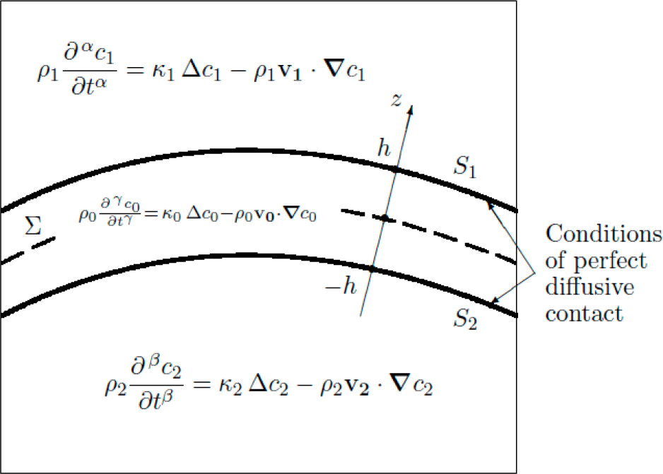
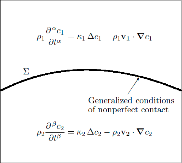
3. Generalized Conditions of Nonperfect Contact

Consider a composite body consisting of three parts: the domain 1, the domain 2, and the intermediate domain designated by the index 0. Matter transport is described by the time-fractional advection diffusion equations appropriate to each domain:

$${\rho }_1\frac{{\partial }^{\alpha }{c}_1}{\partial t^{\alpha }}={\kappa }_1\mathrm{\Delta }{c}_1-{\rho }_1{\mathbf{v}}_1\cdot \nabla c_1,$$

(34)

$${\rho }_2\frac{{\partial }^{\beta }{c}_2}{\partial t^{\beta }}={\kappa }_2\mathrm{\Delta }{c}_2-{\rho }_2{\mathbf{v}}_2\cdot \nabla c_2,$$

(35)

$${\rho }_0\frac{{\partial }^{\gamma }{c}_0}{\partial t^{\gamma }}={\kappa }_0\mathrm{\Delta }{c}_0-{\rho }_0{\mathbf{v}}_0\cdot \nabla c_0.$$

(36)

At the boundary surfaces S₁ and S₁ between the intermediate domain and the corresponding body, the conditions of perfect diffusive contact are fulfilled:

$$c_1|{}_{S_1}=c_0|{}_{S_1},$$

(37)

$$D_{RL}^{1-\alpha }({\kappa }_1\frac{\partial c_1}{\partial n}-{\rho }_1{v}_{(n)1}{c}_1){|}_{S_1}=D_{RL}^{1-\gamma }({\kappa }_0\frac{\partial c_0}{\partial n}-{\rho }_0{v}_{(n)0}{c}_0){|}_{S_1}$$

(38)

and:

$$c_2|{}_{S_2}=c_0|{}_{S_2},$$

(39)

$$D_{RL}^{1-\beta }({\kappa }_2\frac{\partial c_2}{\partial n}-{\rho }_2{v}_{(n)2}{c}_2){|}_{S_2}=D_{RL}^{1-\gamma }({\kappa }_0\frac{\partial c_0}{\partial n}-{\rho }_0{v}_{(n)0}{c}_0){|}_{S_2}.$$

(40)

To investigate the transport processes in such a composite body in the general case is a very complicated problem. When the thickness 2h of the intermediate domain is small with respect to two other sizes and is constant, we can introduce the median surface Σ. Let R₁ and R₂ be the principal radii of curvature of the median surface. If $h/R_1<<1$ and $h/R_2<<1$, then a thin shell is obtained which allows us to reduce a three-dimensional problem in the intermediate layer to a two-dimensional one for the median surface. Thus we introduce the mixed coordinate system (ξ,η,z), where ξ and η are the curvilinear coordinates in the median surface and z is the normal coordinate ( $-h\le z\le h$), see Figure 1.

The time-fractional advection diffusion equation in the intermediate layer (36) is rewritten as:

$${\rho }_0\frac{{\partial }^{\gamma }{c}_0}{\partial t^{\gamma }}={\kappa }_0{\mathrm{\Delta }}_{\mathrm{\Sigma }}{c}_0+{\kappa }_0\frac{{\partial }^2{c}_0}{\partial z^2}-{\rho }_0{\mathbf{v}}_{\mathrm{\Sigma }}\cdot {\nabla }_{\mathrm{\Sigma }}{c}_0-{\rho }_0{v}_{(n)0}\frac{\partial c_0}{\partial z},$$

(41)

where Δ_Σ is the surface Laplace operator, ∇_Σ denotes the surface del operator taking effect along a surface.

Next we average Equation (41) introducing the averaged characteristics of concentration:

$${\mathrm{\Theta }}_1\left(\xi ,\eta ,t\right)=\frac{1}{2h}{\displaystyle \underset{-h}{\overset{h}{\int }}{c}_0(\xi ,\eta ,z,t)}dz,$$

(42)

$${\mathrm{\Theta }}_2\left(\xi ,\eta ,t\right)=\frac{3}{2h^2}{\displaystyle \underset{-h}{\overset{h}{\int }}{c}_0(\xi ,\eta ,z,t)}zdz.$$

(43)

Introducing the averaged characteristics of concentration Θ₁ and Θ₂ is similar to introducing the stress resultants (forces and moments) in the theory of thin elastic shells. The interested reader is referred to the extended literature on this subject (see, for example, [54–57]). From Equation (41) we obtain:

$${\rho }_0\frac{{\partial }^{\gamma }{\mathrm{\Theta }}_1}{\partial t^{\gamma }}={\kappa }_0{\mathrm{\Delta }}_{\mathrm{\Sigma }}{\mathrm{\Theta }}_1-{\rho }_0{\mathbf{v}}_{\mathrm{\Sigma }}\cdot {\nabla }_{\mathrm{\Sigma }}{\mathrm{\Theta }}_1+\frac{{\kappa }_0}{2h}\frac{\partial c_0}{\partial z}{|}_{z=h}-\frac{{\kappa }_0}{2h}\frac{\partial c_0}{\partial z}{|}_{z=-h}-\frac{{\rho }_0{v}_{(n)0}{c}_0}{2h}{|}_{z=h}+\frac{{\rho }_0{v}_{(n)0}{c}_0}{2h}{|}_{z=-h}$$

(44)

$$\begin{array}{l}{\rho }_0\frac{{\partial }^{\gamma }{\mathrm{\Theta }}_2}{\partial t^{\gamma }}={\kappa }_0{\mathrm{\Delta }}_{\mathrm{\Sigma }}{\mathrm{\Theta }}_2-{\rho }_0{\mathbf{v}}_{\mathrm{\Sigma }}\cdot {\nabla }_{\mathrm{\Sigma }}{\mathrm{\Theta }}_2+\frac{3{\rho }_0{v}_{(n)0}}{h}{\mathrm{\Theta }}_1+\frac{3{\kappa }_0}{2h}\frac{\partial c_0}{\partial z}{|}_{z=h}+\frac{3{\kappa }_0}{2h}\frac{\partial c_0}{\partial z}{|}_{z=-h}\hfill \\ -\frac{3{\kappa }_0}{2h^2}{c}_0{|}_{z=h}+\frac{3{\kappa }_0}{2h^2}{c}_0{|}_{z=-h}-\frac{3{\rho }_0{v}_{(n)0}{c}_0}{2h}{|}_{z=h}-\frac{3{\rho }_0{v}_{(n)0}{c}_0}{2h}{|}_{z=-h}\hfill \end{array}$$

(45)

Furthermore, we use the conditions of perfect diffusive contact at the surfaces z=h and z=−h along with the assumption of linear dependence of concentration c₀ on the coordinate z and proceed to the limit h→0 keeping ${\rho }_{\mathrm{\Sigma }}=2h{\rho }_0$, ${\kappa }_{\mathrm{\Sigma }}=2h{\kappa }_0$, $R_{\mathrm{\Sigma }}=2h/{\kappa }_0$ and $v_{\{n)\mathrm{\Sigma }}=v_{(n)0}/(2h)$constant. It should be noted that more general polynomial dependence of the concentration c₀ on the coordinate z or the operator method can also be used (see [58,59]). As a result we obtain the generalized boundary conditions at the median surface Σ (see Figure 2):

$$\begin{array}{l}{\rho }_{\mathrm{\Sigma }}\frac{{\partial }^{\gamma }\left(c_1+c_2\right)}{\partial t^{\gamma }}={\kappa }_{\mathrm{\Sigma }}{\mathrm{\Delta }}_{\mathrm{\Sigma }}\left(c_1+c_2\right)-{\rho }_{\mathrm{\Sigma }}{\mathbf{v}}_{\mathrm{\Sigma }}\cdot {\nabla }_{\mathrm{\Sigma }}\left(c_1+c_2\right)\\ +2\left[D_{RL}^{\gamma -\alpha }\left({\kappa }_1\frac{\partial c_1}{\partial n}-{\rho }_1{v}_{(n)1}{c}_1\right)-D_{RL}^{\gamma -\beta }\left({\kappa }_2\frac{\partial c_2}{\partial n}-{\rho }_2{v}_{(n)2}{c}_2\right)\right],\end{array}$$

(46)

$$\begin{array}{l}{\rho }_{\mathrm{\Sigma }}\frac{{\partial }^{\gamma }\left(c_1-c_2\right)}{\partial t^{\gamma }}={\kappa }_{\mathrm{\Sigma }}{\mathrm{\Delta }}_{\mathrm{\Sigma }}\left(c_1-c_2\right)-{\rho }_{\mathrm{\Sigma }}{\mathbf{v}}_{\mathrm{\Sigma }}\cdot {\nabla }_{\mathrm{\Sigma }}\left(c_1-c_2\right)+6{\rho }_{\mathrm{\Sigma }}{v}_{(n)\mathrm{\Sigma }}\left(c_1+c_2\right)\\ +6\left[D_{RL}^{\gamma -\alpha }\left({\kappa }_1\frac{\partial c_1}{\partial n}-{\rho }_1{v}_{(n)1}{c}_1\right)+D_{RL}^{\gamma -\beta }\left({\kappa }_2\frac{\partial c_2}{\partial n}-{\rho }_2{v}_{(n)2}{c}_2\right)\right]-\frac{12}{R_{\mathrm{\Sigma }}}\left(c_1-c_2\right).\end{array}$$

(47)

When the drift terms are not considered, Equations (46) and (47) reduce to the following equations [7]:

$${\rho }_{\mathrm{\Sigma }}\frac{{\partial }^{\gamma }\left(c_1+c_2\right)}{\partial t^{\gamma }}={\kappa }_{\mathrm{\Sigma }}{\mathrm{\Delta }}_{\mathrm{\Sigma }}\left(c_1+c_2\right)+2\left({\kappa }_1{D}_{RL}^{\gamma -\alpha }\frac{\partial c_1}{\partial n}-{\kappa }_2{D}_{RL}^{\gamma -\beta }\frac{\partial c_2}{\partial n}\right),$$

(48)

$${\rho }_{\mathrm{\Sigma }}\frac{{\partial }^{\gamma }\left(c_1-c_2\right)}{\partial t^{\gamma }}={\kappa }_{\mathrm{\Sigma }}{\mathrm{\Delta }}_{\mathrm{\Sigma }}\left(c_1-c_2\right)+6\left({\kappa }_1{D}_{RL}^{\gamma -\alpha }\frac{\partial c_1}{\partial n}+{\kappa }_2{D}_{RL}^{\gamma -\beta }\frac{\partial c_2}{\partial n}\right)-\frac{12}{R_{\mathrm{\Sigma }}}\left(c_1-c_2\right).$$

(49)

For the classical diffusion equation ( $\alpha =\beta =\gamma =1$) we arrive at the result of Podstrigach [58,59]:

$${\rho }_{\mathrm{\Sigma }}\frac{\partial \left(c_1+c_2\right)}{\partial t}={\kappa }_{\mathrm{\Sigma }}{\mathrm{\Delta }}_{\mathrm{\Sigma }}\left(c_1+c_2\right)+2\left({\kappa }_1\frac{\partial c_1}{\partial n}-{\kappa }_2\frac{\partial c_2}{\partial n}\right),$$

(50)

$${\rho }_{\mathrm{\Sigma }}\frac{\partial \left(c_1-c_2\right)}{\partial t}={\kappa }_{\mathrm{\Sigma }}{\mathrm{\Delta }}_{\mathrm{\Sigma }}\left(c_1-c_2\right)+6\left({\kappa }_1\frac{\partial c_1}{\partial n}+{\kappa }_2\frac{\partial c_2}{\partial n}\right)-\frac{12}{R_{\mathrm{\Sigma }}}\left(c_1-c_2\right).$$

(51)

When the reduced diffusive characteristics of the median surface are equal to zero ( ${\rho }_{\mathrm{\Sigma }}=0$, ${\kappa }_{\mathrm{\Sigma }}=0$, $R_{\mathrm{\Sigma }}=0$, $v_{(n)\mathrm{\Sigma }}=0$), from (46) and (47) we get the conditions of perfect diffusive contact (32) and (33) whereas from (50) and (51) we obtain the conditions of perfect contact (9) and (11).

4. Conclusions

We have analyzed different kinds of boundary conditions for the standard diffusion equation and advection diffusion equation as well for their fractional counterparts. It should be emphasized that due to the generalized constitutive equations for the matter flux the boundary conditions for the time-fractional diffusion equations have their particular traits in comparison with those for the standard ones. The proper physical boundary conditions should be formulated in terms of the matter flux, not in terms of the normal derivative of concentration alone. Specifying the boundary value of the matter flux in the case of the diffusion equation leads to the Neumann boundary condition, but in the case of the advection diffusion equation leads to the Robin boundary condition. The drift parameter v alters the convective mass transfer coefficient H. The transition region between two phases has been considered as a distinct phase having its own reduced characteristics (the reduced mass density ${\rho }_{\mathrm{\Sigma }}$, the reduced diffusive conductivity ${\kappa }_{\mathrm{\Sigma }}$, the reduced diffusive resistance $R_{\mathrm{\Sigma }}$, and the reduced drift parameter $v_{(n)\mathrm{\Sigma }}$ of the median surface), and the generalized conditions of nonperfect contact have been obtained.

References

1. Metzler, R.; Klafter, J. The random walk’s guide to anomalous diffusion: A fractional dynamics approach. Phys. Rep. 2000, 339, 1–77. [Google Scholar]
2. Metzler, R.; Klafter, J. The restaurant at the end of the random walk: recent developments in the description of anomalous transport by fractional dynamics. J. Phys. A Math. Gen. 2004, 37, R161–R208. [Google Scholar]
3. Zaslavsky, G.M. Chaos, fractional kinetics, and anomalous transport. Phys. Rep. 2002, 371, 461–580. [Google Scholar]
4. Magin, R.L. Fractional Calculus in Bioengineering; Begell House Publishers: Redding, CT, USA, 2006. [Google Scholar]
5. Gafiychuk, V.; Datsko, B. Mathematical modeling of different types of instabilities in time fractional reaction-diffusion systems. Comput. Math. Appl. 2010, 59, 1101–1107. [Google Scholar]
6. Uchaikin, V.V. Fractional Derivatives for Physicists and Engineers; Springer: Berlin, Germany, 2013. [Google Scholar]
7. Povstenko, Y. Fractional Thermoelasticity; Springer: New York, NY, USA, 2015. [Google Scholar]
8. Hoffmann, K.H.; Essex, C.; Schulzky, C. Fractional diffusion and entropy production. J. Non-Equilibr. Thermodyn. 1998, 23, 166–175. [Google Scholar]
9. Essex, C.; Schulzky, C.; Franz, A.; Hoffmann, K.H. Tsallis and Rényi entropies in fractional diffusion and entropy production. Physica A 2000, 284, 299–308. [Google Scholar]
10. Li, X.; Essex, C.; Davison, M.; Hoffmann, K.H.; Schulzky, C. Fractional diffusion, irreversibility and entropy. J. Non-Equilibr. Thermodyn 2003, 28, 279–291. [Google Scholar]
11. Cifani, S.; Jakobsen, E.R. Entropy solution theory for fractional degenerate convection-diffusion equations. Annales de l’Institut Henri Poincare (C) Nonlinear Anal 2011, 28, 413–441. [Google Scholar]
12. Magin, R.; Ingo, C. Entropy and information in a fractional order model of anomalous diffusion, Proceedings of the 16th IFAC Symposium on System Identification, Brussels, Belgium, 11–13 July 2011; pp. 428–433.
13. Magin, R.; Ingo, C. Spectral entropy in a fractional order model of anomalous diffusion, Proceedings of the 13th International Carpathian Control Conference, High Tatras, Slovakia, 28–31 May 2012; pp. 458–463.
14. Prehl, J.; Essex, C.; Hoffmann, K.H. Tsallis relative entropy and anomalous diffusion. Entropy 2012, 14, 701–706. [Google Scholar]
15. Prehl, J.; Boldt, F.; Essex, C.; Hoffmann, K.H. Time evolution of relative entropies for anomalous diffusion. Entropy 2013, 15, 2989–3006. [Google Scholar]
16. Magin, R.L.; Ingo, C.; Colon-Perez, L.; Triplett, W.; Mareci, T.H. Characterization of anomalous diffusion in porous biological tissues using fractional order derivatives and entropy. Microporous Mesoporous Mater 2013, 178, 39–43. [Google Scholar]
17. Ingo, C.; Magin, R.L.; Colon-Perez, L.; Triplett, W.; Mareci, T.H. On random walks and entropy in diffusion-weighted magnetic resonance imaging studies of neural tissue. Magn. Reson. Med. 2014, 71, 617–627. [Google Scholar]
18. Ingo, C.; Magin, R.L.; Parrish, T.B. New insight into the fractional order diffusion equation using entropy and kurtosis. Entropy 2014, 16, 5838–5852. [Google Scholar]
19. Zhuang, P.; Liu, F.; Anh, V.; Turner, I. Numerical treatment for the fractional Fokker-Planck equation. ANZIAM J 2007, 48, C759–C774. [Google Scholar]
20. Chen, C.; Liu, F.; Turner, I.; Anh, V. Implicit difference approximation of the Galilei invariant fractional advection diffusion equation. ANZIAM J 2007, 48, C775–C789. [Google Scholar]
21. Liu, F.; Zhuang, P.; Anh, V.; Turner, I.; Burrage, K. Stability and convergence of the difference methods for the space-time fractional advection-diffusion equation. Appl. Math. Comput. 2007, 191, 12–20. [Google Scholar]
22. Liu, F.; Zhuang, P.; Burrage, K. Numerical methods and analysis for a class of fractional advection-dispersion models. Comp. Math. Appl. 2012, 64, 2990–3007. [Google Scholar]
23. El-Sayed, A.M.A.; Behiry, S.H.; Raslan, W.E. Adomian’s decomposition method for solving an intermediate fractional advection-dispersion equation. Comp. Math. Appl. 2010, 59, 1759–1765. [Google Scholar]
24. Golbabai, A.; Sayevand, K. Analytical modelling of fractional advection-dispersion equation defined in a bounded space domain. Math. Comp. Model. 2011, 53, 1708–1718. [Google Scholar]
25. Panday, R.K.; Singh, O.P.; Baranwal, V.K. An analytic algorithm for the space-time fractional advection-dispersion equation. Comp. Phys. Commun. 2011, 182, 1134–1144. [Google Scholar]
26. Saadatmandi, A.; Dehghan, M.; Azizi, M.-R. The Sinc-Legendre collocation method for a class of fractional convection-diffusion equations with variable coefficients. Commun. Nonlinear Sci. Numer. Simulat. 2012, 17, 4125–4136. [Google Scholar]
27. Parvizi, M.; Eslahchi, M.R.; Dehghan, M. Numerical solution of fractional advection-diffusion equation with a nonlinear source term. Numer. Algor. 2015, 68, 601–629. [Google Scholar]
28. Zhang, X.; Huang, P.; Feng, X.; Wei, L. Finite element method for two-dimensional time-fractional Tricomi-type equations. Numer. Methods Partial Differ. Equ. 2013, 29, 1081–1096. [Google Scholar]
29. Yang, Q.; Moroney, T.; Burrage, K.; Turner, I.; Liu, F. Novel numerical methods for time-space fractional reaction diffusion equation in two dimensions. ANZIAM J 2011, 52, C395–C409. [Google Scholar]
30. Jiang, W.; Lin, Y. Approximate solution of the fractional advection-dispersion equation. Comp. Phys. Commun. 2010, 181, 557–561. [Google Scholar]
31. Fu, Z.-J.; Chen, W.; Yang, H.-T. Boundary particle method for Laplace transformed time-fractional diffusion equations. J. Comput. Phys. 2013, 235, 52–66. [Google Scholar]
32. Sun, H.G.; Zhang, Y.; Chen, W.; Reeves, D.M. Use of a variable-index fractional-derivative model to capture transient dispersion in heterogeneous media. J. Contaminant Hydrol 2014, 157, 47–58. [Google Scholar]
33. Chen, W.; Sun, H.; Zhang, X.; Korošak, D. Anomalous diffusion modeling by fractal and fractional derivatives. Comp. Math. Appl. 2010, 59, 1754–1758. [Google Scholar]
34. Gafiychuk, V.; Datsko, B.; Meleshko, V.; Blackmore, D. Analysis of the solutions of coupled nonlinear fractional reaction-diffusion equations. Chaos Solitons Fractals 2009, 41, 1095–1104. [Google Scholar]
35. Povstenko, Y. Different kinds of boundary conditions for time-fractional heat conduction equation, Proceedings of the 13th International Carpathian Control Conference, High Tatras, Slovakia, 28–31 May 2012; pp. 588–591.
36. Povstenko, Y.Z. Fractional heat conduction in infinite one-dimensional composite medium. J. Therm. Stresses 2013, 36, 351–363. [Google Scholar]
37. Povstenko, Y. Fractional heat conduction in an infinite medium with a spherical inclusion. Entropy 2013, 15, 4122–4133. [Google Scholar]
38. Podstrigach, Y.S.; Povstenko, Y.Z. Introduction to the Mechanics of Surface Phenomena in Deformable Solids; Naukova Dumka: Kiev, Ukraine, 1985; In Russian. [Google Scholar]
39. Kaviany, M. Principles of Heat Transfer in Porous Media; Springer: NewYork, NY, USA, 1995. [Google Scholar]
40. Feller, W. An Introduction to Probability Theory and Its Applications; John Wiley & Sons: New York, NY, USA, 1971. [Google Scholar]
41. Scheidegger, A.E. The Physics of Flow through Porous Media; University of Toronto Press: Toronto, Canada, 1974. [Google Scholar]
42. Van Kampen, N.G. Stochastic Processes in Physics and Chemistry; North-Holland: Amsterdam, The Netherlands, 1981. [Google Scholar]
43. Risken, H. The Fokker-Planck Equation; Springer: Berlin, Germany, 1989. [Google Scholar]
44. Nield, D.A.; Bejan, A. Convection in Porous Media; Springer: New York, NY, USA, 2006. [Google Scholar]
45. Povstenko, Y.Z. Fractional heat conduction equation and associated thermal stresses. J. Therm. Stresses 2005, 28, 83–102. [Google Scholar]
46. Povstenko, Y.Z. Thermoelasticity which uses fractional heat conduction equation. J Math. Sci 2009, 162, 296–305. [Google Scholar]
47. Povstenko, Y.Z. Theory of thermoelasticity based on the space-time-fractional heat conduction equation. Phys. Scr. 2009, 136, 014017. [Google Scholar]
48. Povstenko, Y.Z. Fractional Cattaneo-type equations and generalized thermoelasticity. J. Therm. Stresses 2011, 34, 97–114. [Google Scholar]
49. Povstenko, Y. Non-axisymmetric solutions to time-fractional diffusion-wave equation in an infinite cylinder. Fract. Calc. Appl. Anal. 2011, 14, 418–435. [Google Scholar]
50. Gorenflo, R.; Mainardi, F. Fractional calculus: integral and differential equations of fractional order. In Fractals and Fractional Calculus in Continuum Mechanics; Carpinteri, A., Mainardi, F., Eds.; Springer: New York, NY, USA, 1997; pp. 223–276. [Google Scholar]
51. Podlubny, I. Fractional Differential Equations; Academic Press: San Diego, CA, USA, 1999. [Google Scholar]
52. Kilbas, A.A.; Srivastava, H.M.; Trujillo, J.J. Theory and Applications of Fractional Differential Equations; Elsevier: Amsterdam, The Netherlands, 2006. [Google Scholar]
53. Povstenko, Y. Theory of diffusive stresses based on the fractional advection-diffusion equation. In Fractional Calculus: Applications; Abi Zeid Daou, R., Moreau, X., Eds.; NOVA Science Publishers: New York, NY, USA, 2015; pp. 227–241. [Google Scholar]
54. Goldenveiser, A.L. Theory of Thin Shells; Pergamon Press: Oxford, UK, 1961. [Google Scholar]
55. Naghdi, P.M. The theory of shells and plates. In Handbuch der Physik; Truesdell, C., Ed.; Springer: Berlin, Germany, 1972; pp. 425–640. [Google Scholar]
56. Vekua, I.N. Some General Methods of Constructing Different Variants of Shell Theory; Nauka: Moscow, Russia, 1982; In Russian. [Google Scholar]
57. Ventsel, E.; Krauthammer, T. Thin Plates and Shells: Theory, Analysis, and Applications; Marcel Dekker: New York, NY, USA, 2001. [Google Scholar]
58. Podstrigach, Ya.S. Temperature field in a system of solids conjugated by a thin intermediate layer. Inzh.-Fiz. Zhurn 1963, 6, 129–136, In Russian. [Google Scholar]
59. Podstrigach, Ya.S.; Shvetz, R.N. Thermoelasicity of Thin Shells; Naukova Dumka: Kiev, Ukraine, 1978; In Russian. [Google Scholar]
Figure 1. Thin intermediate layer between two media.
Entropy 17 04028f1
Figure 2. A contact surface Σ having its own physical characteristics.
Entropy 17 04028f2