1. Introduction
1.1. Motivation
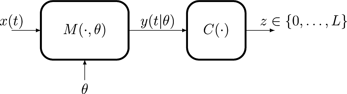
The paper presents a new density estimator motivated by problems of population modeling, where the interest is in estimating the probability distribution πθ, θ ∈ Θ, of the parameters of a mathematical model M(·|θ) characterizing the response y(t|θ) of individuals to applied stimuli x(t). The ultimate goal is in general to be able to predict the dispersion of the response of the population to an arbitrary future stimulus x(t), rather than to make a “tomography” of the population itself. These types of problems are frequent in domains like biomedical engineering, insurance studies or environmental management.
If the parameter
θ can be estimated from each observation
y(
t|θ) and each individual’s parameter is chosen independently from
πθ, the problem of estimating
πθ from a collection of responses
is formally equivalent to the usual density estimation problem from a set of independent and identically distributed samples
and can be solved using standard parametric or non-parametric methods; see the abundant literature on non-linear mixed-effects models. The situation considered in this paper is more complex, in that the response
y(
·|θ) of the model not observable, and we only have access to the result of the classification of its assignment to a finite number (
L + 1) of possible labels by a known classifier
C(·).
Figure 1 illustrates the structural modeling/observation framework that we consider.
In this setup, each observation can no longer be related to a single point θ ∈ Θ, the same label z being assigned, for the same stimulus x(t), to all responses inside a subset R ⊂ Θ. The set R is completely determined by the pair (z, x(t)) together with knowledge of the model M(·|θ) and of the classifier rule C(·). This situation, when a single observation does not give information with respect to the individual value θ, but only the indication that it belongs to a set, is commonly known in the statistical literature as “censored observations”. While in general studies of the density estimation under censored observations have assumed that the censoring sets R are intervals, the geometry of our censoring regions is determined by the structure of the (possibly highly non-linear) operators M(·|θ) and C(·) and can have an arbitrary morphology, requiring modification of the existing methods.
In Section 4, we detail a particular instance of the problem formally presented above, relevant in the context of the prevention of decompression sickness in hyperbaric diving. Readers may want to read the material in Section 4.1 to have a concrete instantiation of the generic stimuli and operators used in the presentation above.
1.2. Notation and Problem Formulation
Consider the notation introduced in Section 1.1 (see also
Figure 1), and let
denote the available set of observations, where label
zn ∈ {0, …,
L} has been observed for input
X(n) = {
xn(
t),
t ∈
Tn}, where
Tn is the duration of the stimulus. Denote by
Rn ⊂ Θ the set of all individual parameters whose response to
X(n) receives label
zn:
We assume that for all possible stimuli X(n), the composition C(M(X(n)|·)) (of the model and the classifier) is a measurable function from Θ to {0, …, L} with respect to the restriction of the Lebesgue measure to the set Θ. Under this assumption, the probability of the sets
is well defined for all 0 ≤ ℓ ≤ L and all stimuli for any distribution absolutely continuous with respect to the Lebesgue measure.
Usually, in population studies, the same stimulus is applied to several individuals. We assume here that stimuli
X(j) are chosen in a finite set
Each possible input function
X(j) in
determines a partition of Θ in
L + 1 sets, that we denote by
:
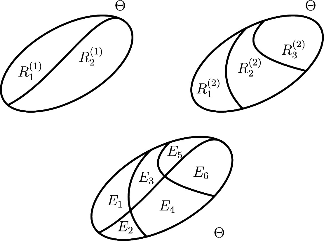
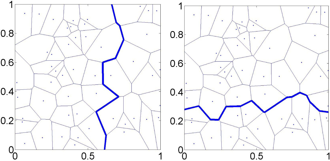
The top row of
Figure 2 illustrates schematically partitions that correspond to classification in two (
L1 = 1) and three (
L2 = 2) classes of the response to two distinct stimuli.
Let
nj be the number of times that stimulus
X(j) has been used in the
N observations and
the number of times label
ℓ occurred in these
nj experiences. The observed dataset determines
J empirical laws
, each one associated with a distinct partition
:
When we want to emphasize the number of observations on which these empirical laws are based, we will call
an nj-type. With the notation defined above, we can finally state the problem addressed in this paper with full generality.
Problem 1. (Density estimation from region-censored data)
Find the non-parametric estimate of πθ from the set of J nj-types,
j = 1, …,
J (see Equation (1)) of the discrete random variables associated with the known partitions (see Equation (4)). Before initiating the study of this estimation problem, we show below how a set of constraints can be related to the observations (1) leading to an alternative problem formulation.
Let 1
A(
θ) be the indicator function of set
A ⊂ Θ and
the (non-observed) empirical distribution:
where
,
i = 1, …,
nj, is the parameter of the
i-th individual to whom stimulus
X(j) has been applied. It is immediate that
in
Equation (1) can be written as the statistical expectation of the indicator function of
with respect to
:
We stress that in our context, the (virtual) datasets
are distinct for different values of j ∈ {1, …, J}, since they correspond to statistically-independent samples from πθ.
The remarks above allow us to relate Problem 1 to two alternative problems: Problem 2 formulated below and Problem 3 presented in the next subsection.
Problem 2. (Density estimation under moment constraints)
Consider a set of partitions (j),
j ∈ {0 …
L}
all of size L+1,
and let,
with M = (
L+1)
J, be the set of indicator functions.
Denote by,
m = 1, …,
M, the corresponding empirical moments as in (2). Find the non-parametric estimate of πθ that satisfies the set of constraints: Note that the existence and unicity of the solution to this problem is not guaranteed: depending on the set of partitions and empirical moments, the problem may have no solution or admit a solution (possibly non-unique).
The next subsection summarizes the present background on the two problems formulated above. Prior to that, we present three definitions that will be useful in the sequel.
Definition 1. Let be the smallest partition of Θ whose generated σ-algebra,
, contains all partitions (elements of are the minimal elements of the closure of the union of all partitions with respect to set intersection). The size is necessarily finite. We denote by Em, m ∈ {1, …, Q} a generic element of.
The bottom row of
Figure 2 shows the partition
generated by the two partitions in the top.
Definition 2.
is the set of elements of that intersect,
such that: Definition 3. Let πθ be a probability distribution over Θ
and a finite partition of Θ.
We denote byπθ,Q the probability law induced by πθ over the elements of:
1.3. Background
1.3.1. Density Estimation from Region-Censored Data
Determination of
, the NPMLE (non-parametric maximum likelihood estimate) of
πθ from censored observations,
i.e., the solution of Problem 1, has been studied by many authors, starting with the pioneering formulation of the Kaplan–Meier product-limit estimator [
1]. Several types of censoring (one-sided, interval,
etc.) have been considered since, first for scalar and more recently for multivariate distributions.
The problem assessed here departs from previous studies in that our (multi-dimensional) censoring regions
⊂ Θ can have arbitrary geometry. To emphasize this, we speak of “region-censoring”, instead of the more common term “interval-censoring.” Another important difference concerns the fact that our regions are elements of a known set of partitions, being in general observed several times, while in general, no relation between the censoring intervals is assumed in the literature, each one being usually applied once.
Several facts are known about the NPMLE for censored observations.
Proposition 1.
The support of,
i
s confined to a finite number K ≤ Q of elements of,
the so-called “elementary regions”:
This set necessarily has a non-empty intersection with all observed lists,
i.e.,
all distributions that put the same probability mass wk = {πθ(Ek)}, k = 1, …, K in the elementary regions have the same likelihood;
there is in general no unique assignment of probabilities that maximizes the likelihood.
Turnbull [
2] has first demonstrated (i) giving an algorithm to find the pairs
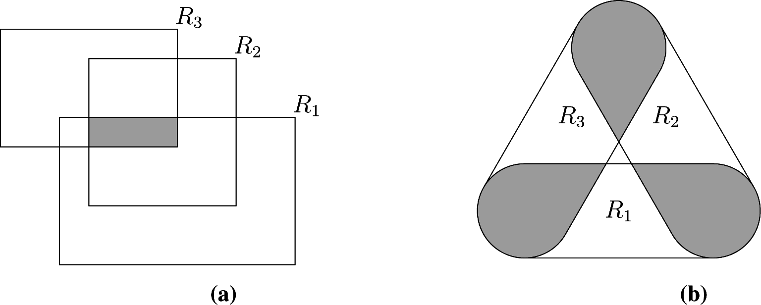
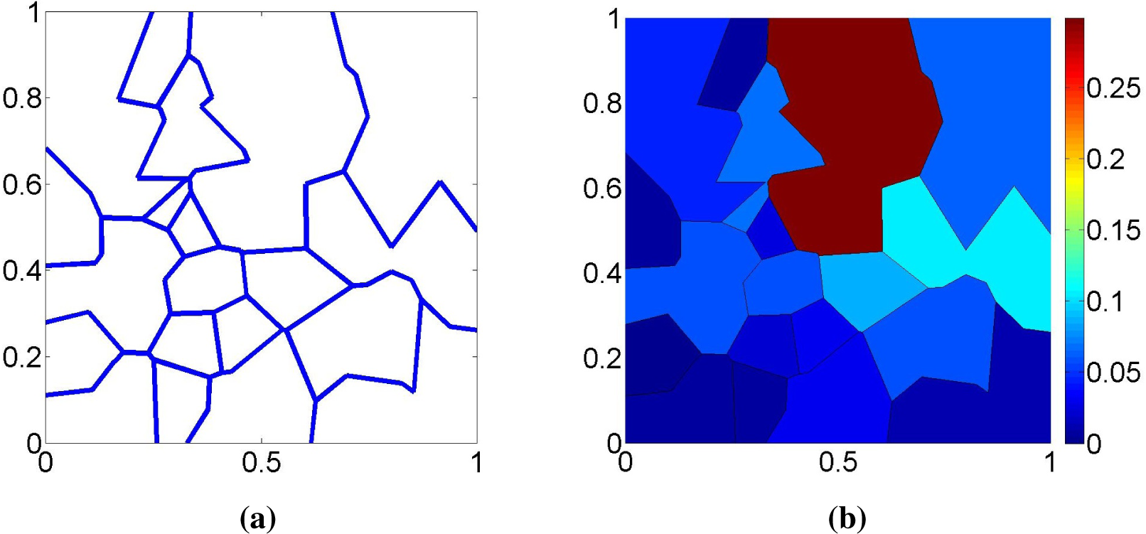
for the scalar case. Gentleman and Vandal [
3] addressed the multivariate interval-censored case, showing that the
Ek’s are the intersections of the elements of the maximal cliques of the intersection graph of the set of observed intervals; see
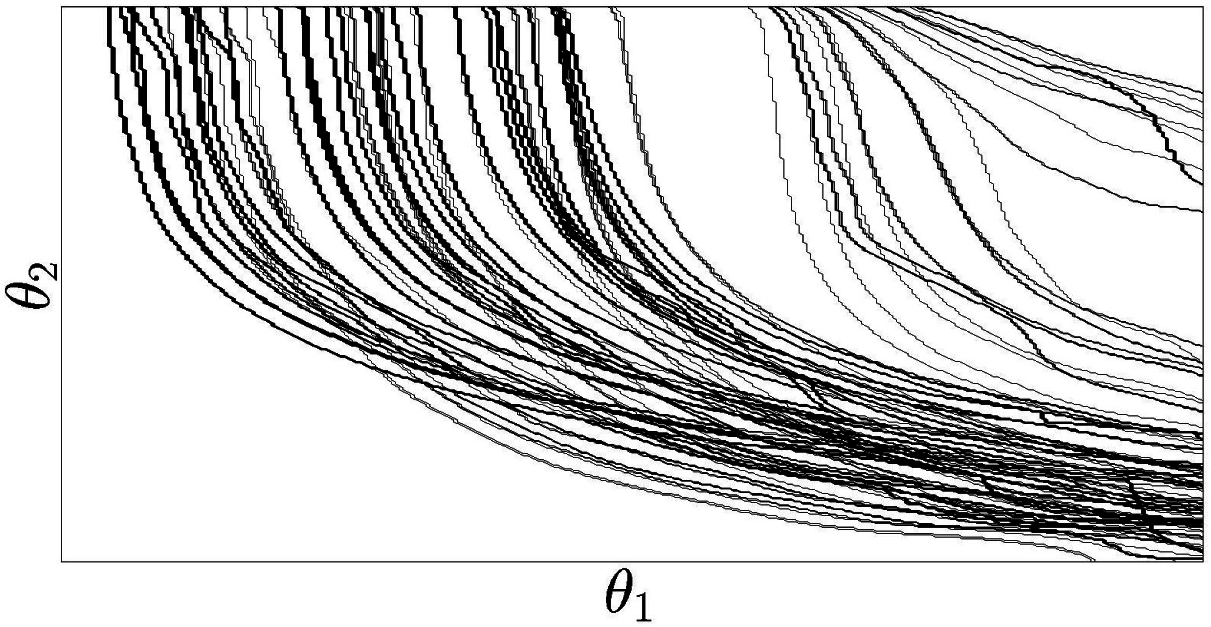
Figure 3a for a bi-dimensional example. We have shown elsewhere [
4] that (i) also holds when the censoring sets have arbitrary geometry, but that some elementary regions are now associated with non-maximal cliques of the intersection graph, as shown in
Figure 3b, requiring a slightly more complex identification of the sets
Ek, which we do not detail here.
Facts (i) and (ii) together imply that the NPMLE problem can be studied in the
K-dimensional probability simplex
, since
is determined only up to the probability vector
ŵ = {
ŵ1, …,
ŵK}. The two types of “non-uniqueness” of the NPMLE, (ii) and (iii), have been first pointed out by Turnbull [
2]. More recently, they were studied in detail for the multi-variate case in [
3], where the authors coined the terms representational (ii) and mixture (iii) non-uniqueness, further showing that the set of probability laws
defining NPMLEs is a polytope.
The NPMLE under censored observations retains the typical consistency properties of the maximum likelihood estimates, in particular
tends to
πθ,(j) (
ℓ) (see
Equation (4)) when
nj → ∞. It is not possible to guarantee the consistency of the estimate of the distribution of
over the finer partition
. However, the simulations studies presented in Section 3 show that as the number of partitions
J tends to infinity and this
σ-algebra gets finer, while keeping fixed each
nj (and thus,
n →
∞ with
J), the distance between the true and estimated probability laws decreases to zero.
Facts (i)–(iii) seriously hinder application of NPMLEs in many domains, in particular when, as is the case in our study, they provide a model of the diversity of the population under analysis that will be used for subsequent risk assessment. Besides being affected by some degree of arbitrariness (Facts (ii) and (iii)), the concentration of the probability mass in a small number of bounded regions reveals a tendency to underestimate population diversity, which may result in strong biases when estimating risk under unobserved stresses. The simulation studies that will be presented in Section 4 illustrates to what extent a lack of identifiability and a tendency to concentrate its support compromise the ability to predict the empirical laws corresponding to stimuli that were not used in the available dataset.
1.3.2. Density Estimation under Moment Constraints
Eventual non-unicity problems in density estimation under constraints on moments, like Problem 2, have been most often solved by relying on the maximum entropy (MaxEnt) principle [
5] to select the most un-informative density that can match the observed moments
. Several information entropies have been considered in this context, the original Shannon entropy
H1(·) remaining the most commonly used due to its simple interpretation in terms of coding theory and its intimate link to fundamental results in estimation theory, while amongst generalized entropies, the Rényi entropy
Hα(·), coinciding with Shannon when
α → 1, is often chosen due to its appealing numerical and analytical tractability for
α = 2:
Problem 3. (H-MaxEnt density estimator)
Let H(·)
be a generalized entropy. The H-MaxEnt estimate of Problem 2 is the solution of: When
is non-empty (i.e., the constraints are compatible) the MaxEnt density can be analytically determined for some choices of H(·).
Proposition 2. (Equivalence to ML estimation in the exponential family)
Assume that the constraints of Problem 2 are statistical averages with respect to the empirical distribution of a common dataset,
i.e.,
in Equation (2), such that: Note that the
H1-MaxEnt/ML equivalence is lost when the empirical averages
are not all obtained from the same dataset, as is the case in our problem, where (see
Equation (2)) constraints associated with distinct stimuli are being derived from distinct empirical distributions.
When the constraints are not compatible, i.e.,
and Problem 2 has no solution,
is not defined, and only a relaxed version of the original problem can be solved.
Problem 4. (Relaxed H–MaxEnt density estimator)
Let H be a generalized entropy, and ϵ ∈ ℝ
+M. The -relaxed H-MaxEnt density estimate is the solution of:where g is the M-dimensional vector function with m-th component gm(·),
is the M-dimensional vector of empirical expectations of g, ║·║
π is a vector of norms depending on π and inequality is understood component-wise. This estimator has been studied in detail in [
8,
9] for the Shannon entropy and moment constraints derived from a single empirical distribution, where the authors fully exploit the equivalence between regularized MaxEnt as formulated above and
ℓ1-penalized maximum likelihood in the exponential family, showing that Proposition 2 holds in a more generic sense.
Proposition 3. (Equivalence of ℓ1-regularized H1-MaxEnt and penalized log-likelihood [9]) Problem 4 with H =
H1 (Shannon entropy) and ║·║
π the ℓ1 norm for the expected value:where the constraintsare empirical averages computed using a dataset Θ,
is equivalent to the maximization of the sum of the log-likelihood of Θ
for the exponential family (6) penalized by the term,
where ϵm is the m-th element of ϵ.
By linking the relaxation level (the parameter in Problem 4) to the expected level of accuracy of the empirical averages
, in [
8,
9], the authors are able to establish performance guarantees for the resulting density estimate, in terms of log-likelihood loss.
As before, this regularized-MaxEnt/penalized-ML equivalence only holds when all constraints are on the empirical moments with respect to the same underlying empirical distribution. This is not true in population analysis, where an individual is observed only through one of the partitions, and we cannot invoke the properties of maximum likelihood estimators to characterize the properties of regularized MaxEnt estimators, as is done in [
8].
We remark that the regularized MaxEnt estimates are unique for strictly concave entropy functionals and always exist for sufficiently large ϵ. They do not suffer from neither representational non-unicity, the optimal continuous distribution being constant inside each element of
, nor from mixture non-uniqueness, being the solution of a concave criterion under linear inequality constraints.
1.4. Contributions
As largely documented in the literature, the NPMLE using censored data frequently exhibits a singular behavior. By concentrating probability mass in a subset of Θ of a small Lebesgue measure, they favor “over-homogenous” population models that may lead to dangerous biases in the context of risk assessment, by masking the existence of individuals for which risk can be large. As shown above, the problem of density estimation from censored observations addressed in the paper can be recast as the problem of density estimation under a set of constraints derived from the censored observations, each constraint being associated with one of the censoring regions.
While MaxEnt has been frequently used for density estimation from the joint observation of empirical moments of a set of features, its use for region-censored data arising from strongly quantified data, as we consider in this paper, violates the conditions under which previous equivalence to maximum likelihood estimation in the Gibbs family can be established. In these circumstances, guarantees on the likelihood of the original data can be no longer given.
We propose a novel estimator that explicitly relies on the two criteria, the most likely maximum entropy estimator (MLME), where the degree of regularization of a MaxEnt estimate (i.e., of the solutions to Problem 4) is chosen such that the resulting estimate has maximum likelihood. The duality of the two criteria is exploited to allow suppression of singularities that are due to inconsistent or small datasets, and the resulting solution converges to the non-parametric maximum likelihood solution as the size of the datasets associated with each constraint (censoring region) grows. By using the Rényi entropy of order two instead of the Shannon entropy, we are led to a quadratic optimization problem with linear inequality constraints that has an efficient numerical implementation.
While no theoretical performance guarantees are given, the paper presents numerical studies of the performance of the proposed MLME estimator in real and simulated data, comparing it to the NPMLE and to the best fitting MaxEnt solutions. The results of cross-validation on a real dataset show that our novel estimator is better than the NPMLE or the minimally-regularized MaxEnt estimator, leading to better predictions of the population risk under unobserved stress conditions.
The paper is organized as follows. Section 2 illustrates the poor behavior of the NPMLE using simulated data. We show (Section 2.4) that even the most uncertain of the NPMLEs still presents singularities that are unlikely to occur in a natural population. The section starts by presenting the likelihood function and defining the polytope of NPMLE solutions. It also addresses the numerical determination of the NPMLE, and two optimization algorithms are presented.
Section 3 presents the main contribution of the paper, introducing the most likely Rényi MaxEnt estimator (MLME; see Definition 4). We compare our estimator to the NPMLE, demonstrating using simulated datasets that it performs better. We also present numerical studies of its asymptotic behavior as the number J of different stimuli becomes large, revealing a remarkably better behavior.
In Section 4, the proposed estimator is applied to the real problem that motivated this study, in the context of the prevention of decompression sickness in hyperbaric deep sea diving. The new estimator is compared to classical maximum likelihood and maximum entropy estimators on real and simulated data, illustrating the superior performance of the new estimator in a realistic situation.
3. Most Likely Rényi-MaxEnt
To avoid the singular behavior of the NPMLE, we must estimate πθ with a criterion other than maximum likelihood. Relying on the link of our problem with density estimation under constraints, we propose to estimate πθ through the maximum entropy principle.
If there exists a
π that can satisfy all constraints,
i.e., if there exists a solution to Problem 2, the corresponding
w belongs to the NPMLE polytope
. However, being derived from
J distinct empirical distributions, the
J constraints are in general inconsistent, and as in [
9], we consider entropy maximization under relaxed constraints,
i.e., Problem 4. For reasons of numerical efficiency, we consider the Rényi entropy
H2.
Problem 5. (Relaxed ME estimator)
For ϵ ∈ ℝ
+, define the -relaxed MaxEnt estimator as:where ∑
(j) is the covariance of the empirical estimate and is obtained from f(j) by retaining all but one of its non-zero elements. We remark that the constraints in Problem 5, the relaxed MaxEnt problem that we solve, take into account the correlation between the observed frequencies, contrary to what is done in [
9], where the degrees of relaxation of each constraint are fixed independently, as in Problem 4. As we will verify in Section 4 (see also the discussion around
Figure 8), use of an inappropriate metric in the constraints directs the estimator towards sets of solutions that have have lower likelihood, resulting in a poor ability to reproduce the observed empirical moments.
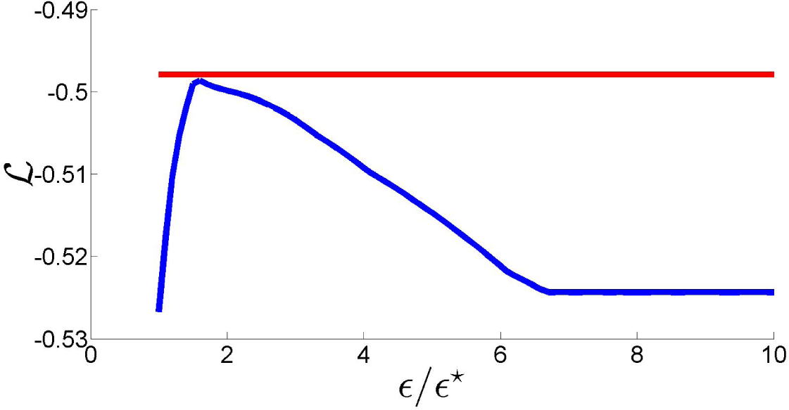
Denote by
ϵ⋆ ≥ 0 the smallest value of
ϵ for which there exists a solution to Problem 5. Since in (13) we use the
ℓ∞ metric to evaluate the deviation of a model
π with respect to the empirical moments and
ℓ∞ is not equivalent to the (Riemannian) metric induced by maximum likelihood in the simplex
, we cannot guarantee that likelihood is monotonically decreasing with the degree of relaxation,
i.e., that
, for
ϵ >
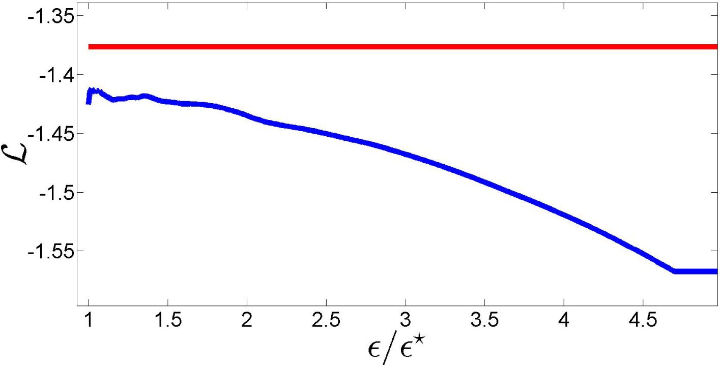
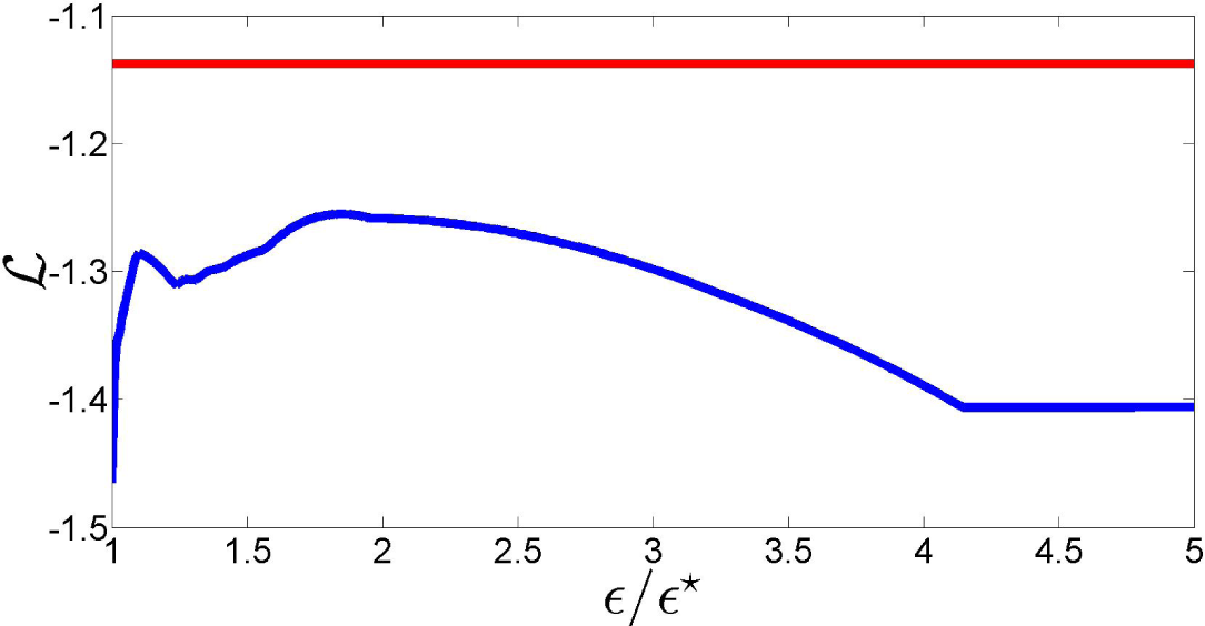
ϵ⋆. In fact, as the plot of the log-likelihood of
as a function of
ϵ/ϵ⋆ in
Figure 7 shows, this is not necessarily true for values of
ϵ close to
ϵ⋆. More importantly, this figure shows that a suitable choice of the relaxation term can lead to a likelihood loss with respect to the NPMLE that is minimal, improving the fit to the data. These remarks motivate the definition of the new estimator proposed in this paper.
Definition 4. (MLME: the most likely MaxEnt estimator)
Let denote the solution of Problem 5 for a generic ϵ ≥
ϵ⋆. The most likely Rényi-MaxEnt estimator is: Proposition 5. (ϵ⋆ = 0)
If ϵ⋆ = 0, then the feasible set of the constrained optimization Problem 5 coincides with the NPMLE polytope. Since the likelihood of all solutions with ϵ > 0 will be smaller, the MLME estimate coincides in this case with the MaxEnt NPMLE:.
Since the probability that
ϵ⋆ = 0 is small for finite datasets, the solution space of our constrained optimization problem is in general larger than the NPMLE polytope
. We illustrate now the geometry of the NLME
using the following simple example for which
L = 1,
J = 2,
K = 3 and:
This choice allows us to represent graphically the elements of
; see
Figure 8. The empirical moments (
,
,
,
) have been chosen such that the constraints are incompatible, avoiding the trivial case where
,
and
all coincide.
Figure 8 illustrates in
the geometry behind the MLME. Black lines
and
correspond to the constraints, which do not intersect since they are incompatible. For this example, the NPMLE (orange dot on the boundary of
, its second component being zero) is unique. All distributions that satisfy the minimally-relaxed constraints (
i.e., with
ϵ =
ϵ⋆) belong to the two gray areas, their intersection defining
(the green dot, also on the boundary of
). The dashed green line is the curve defined by
in
for
ϵ ≥
ϵ⋆, which has an accumulation point in the uniform distribution
as
ϵ becomes sufficiently large for the uniform distribution to satisfy the constraints. Our estimator MLME is the point in this green curve at which the value of the likelihood is the largest, that is the highest level set of the likelihood function over
whose intersection with the green curve is a single point. The orange curve shows this level set, the contact point (red dot) being the MLME
.
The MLME estimator
corresponds in general to an
ϵ >
ϵ⋆ in the constraints (13). In terms of vector w of probabilities of the elementary regions
Ek, this set is a polytope
, defined by its linear boundaries, which characterizes all solutions compatible with the data. One may notice that although the determination of its vertices is a difficult task, approximation of
by the maximum-volume interior ellipsoid is feasible at a reasonable computational cost [
19], providing directly a lower bound on the volume of
.
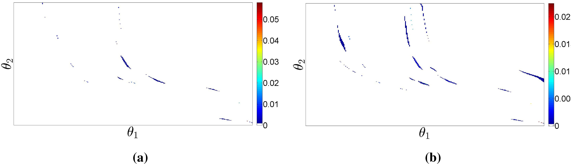
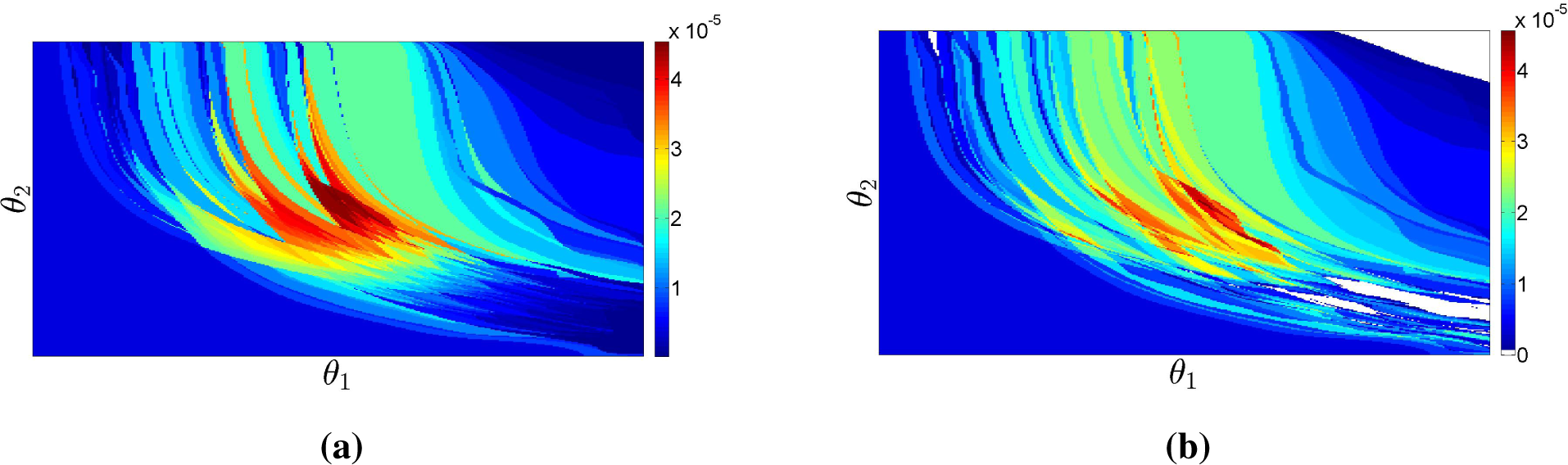
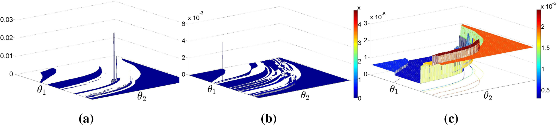
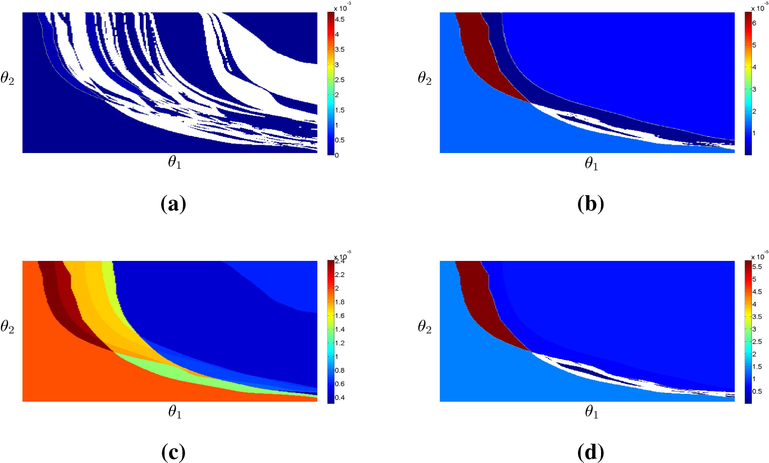
Figure 9 shows the proposed estimator
for the same dataset as in
Figure 6. Note that the distribution of the probability mass is much smoother than in
Figure 6 and that the support of
is now the entire Θ. This example shows that the new estimator
is able to exploit the dual characteristics of the ML and MaxEnt criteria to produce an estimate that is not too informative while still fitting the observed data reasonably well.
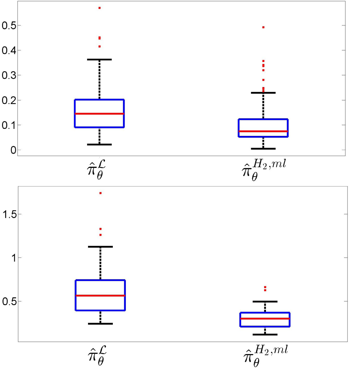
Two common measures of the difference between two distributions are the Kolmogorov and the total variation distances. The Kolmogorov distance
dK is the maximum value of the absolute difference between the two cumulative distributions, while the total variation distance
dTV is the sum of all absolute differences [
20].
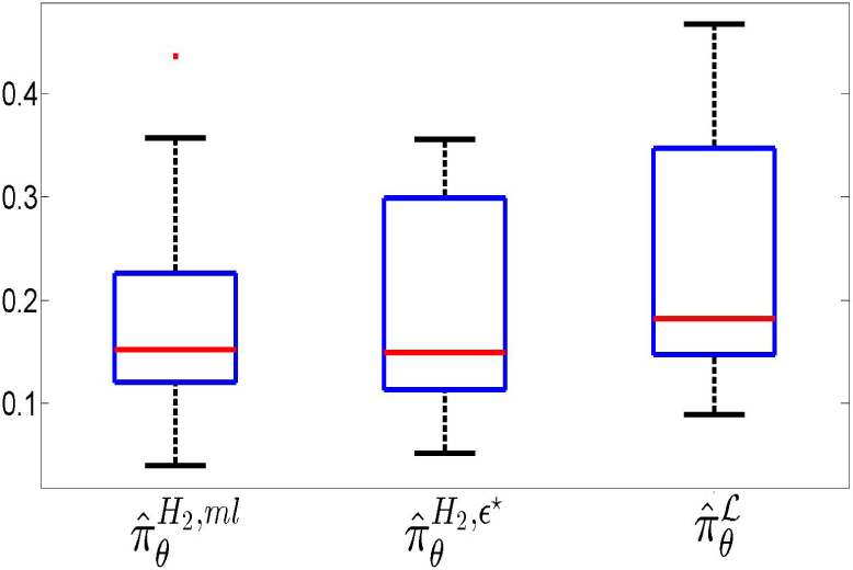
Figure 10 addresses the performance of the estimation of the true probability law over
, showing box-plots of the Kolmogorov–Smirnov (left) and total variation (right) distances between
and the NPMLE and the MLME estimates observed in 200 simulations, each for
N = 10
3 observations. In each plot, the box in the left corresponds to the MaxEnt-NPMLE estimator
and the one on the right to the the proposed estimator
. This clearly demonstrates the superiority of the estimator proposed in the paper. Note that the difference is more pronounced for the total variation, which is the criterion that best indicates the predictive power of the identified population model.
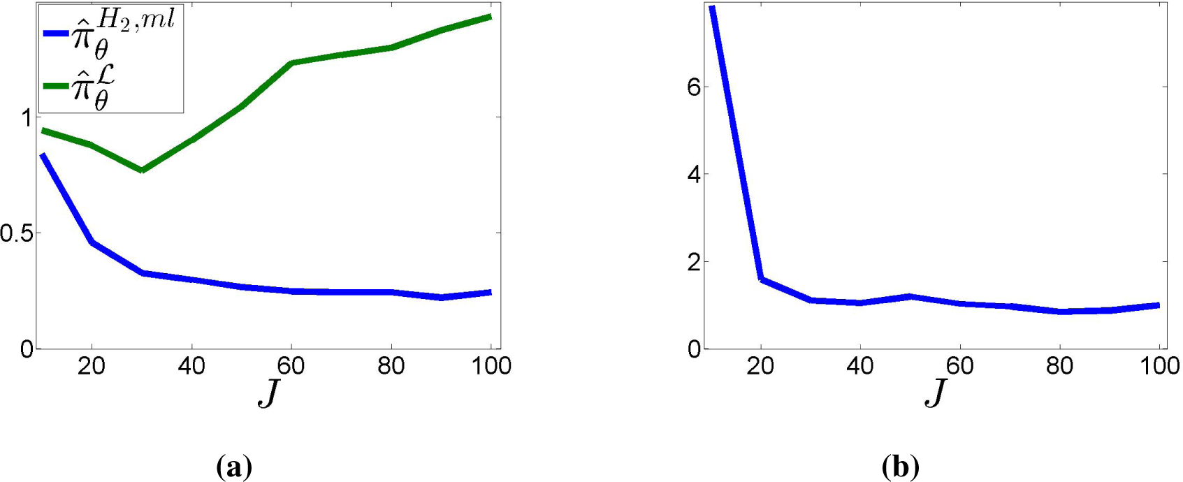
Finally,
Figure 11 shows the behavior under an increasing number of randomly-generated binary partitions. The total number of observations grows with
J:
N = 100
J. The plots show the empirical average of the two Kullback–Leibler divergences
D(·║
πθ) (
Figure 11a) and
D(
πθ║·) (
Figure 11b) over 100 randomly-generated datasets for each value of
J, with
J varying from 10 to 100 in steps of 10. Here, the probability of “dangerous” partitions has been increased to 10
−2, to guarantee a sufficient number of samples censored by them.
Figure 11a suggests that
may be consistent, which is strongly contradicted by the behavior observed for the NPMLE. The divergence
was infinite in all simulations (due to
for some
Ek ∈
) and, thus, cannot be presented in
Figure 11b.


