Article

Nonlinear Stochastic Control and Information Theoretic Dualities: Connections, Interdependencies and Thermodynamic Interpretations

1
The Daniel Guggenheim School of Aerospace Engineering, Georgia Institute of Technology, Atlanta,GA 30332-0150, USA
2
Institute of Robotics and intelligent Machines, Georgia Institute of Technology, Atlanta, GA30332-0150, USA 
Entropy 2015, 17(5), 3352-3375; https://doi.org/10.3390/e17053352
Submission received: 2 February 2015 / Revised: 21 April 2015 / Accepted: 29 April 2015 / Published: 15 May 2015

Abstract

:
In this paper, we present connections between recent developments on the linearly-solvable stochastic optimal control framework with early work in control theory based on the fundamental dualities between free energy and relative entropy. We extend these connections to nonlinear stochastic systems with non-affine controls by using the generalized version of the Feynman–Kac lemma. We present alternative formulations of the linearly-solvable stochastic optimal control framework and discuss information theoretic and thermodynamic interpretations. On the algorithmic side, we present iterative stochastic optimal control algorithms and applications to nonlinear stochastic systems. We conclude with an overview of the frameworks presented and discuss limitations, differences and future directions.

1. Introduction

While the topic of nonlinear stochastic control has been traditionally studied within control and applied mathematics, over the past 10–15 years, there has been an increasing interest by researchers in machine learning and robotics communities to expand nonlinear stochastic optimal control in terms of theoretical generalizations and algorithms. The main motivation for this increasing interest is the ability to solve stochastic optimal control problems with forward sampling of stochastic differential equations (SDEs). There have been a few approaches in the literature on this topic, called path integral (PI) control [13], Kullback–Leibler (KL) control or linearly-solvable control [4,5].
The PI control framework is derived for continuous time stochastic systems affine in controls and noise and for finite horizon optimal control problems. In the KL control, the derivation is in discrete time Markov decision processes (MDPs) and includes finite horizon, infinite horizon, exponentially-discounted and first exit optimal control problems. The continuous time equivalent of the KL control is recovered when transition probabilities are defined based on the corresponding SDEs. Due the central role that linear partial differential equations (PDEs) play in the analysis of the aforementioned approaches, we will refer to them as linearly-solvable optimal control (LSOC), and when necessary, we will use the explicit names of PI or KL control. Moreover, we will restrict our analysis to the finite horizon case. Similar connections have been identified for the infinite horizon case [6]. The analysis for the infinite horizon case will be presented in a follow-up manuscript.
One of the important findings in the LSOC framework is the observation that under certain conditions related to the process noise and control authority, stochastic optimal control problems can be solved with forward sampling of SDEs and the evaluation of expectations. The fundamental theorem that made this observation possible, especially for the continuous case, is the Feynman–Kac lemma [79]. The Feynman–Kac lemma connects SDEs and linear backward PDEs by providing a probabilistic representation of solutions of backwards PDEs. Alternative computational algorithms to the sampling-based LSOC framework incorporate methods on low rank tensor approximation to find solution of linear PDEs on a domain of interest [10].
With the goal to unify different views on stochastic optimal control as developed within different disciplines in sciences and engineering, this work aims to present recent developments and to discuss their connections with previous work using information theoretic concepts. In particular, we expand upon our previous work on this topic [11] and present connections between the LSOC framework as presented within the machine learning and statistical physics communities with the information theoretic view of nonlinear stochastic optimal control theory using the free energy-relative entropy relationship [1215].
Below, we summarize the main points of our analysis:
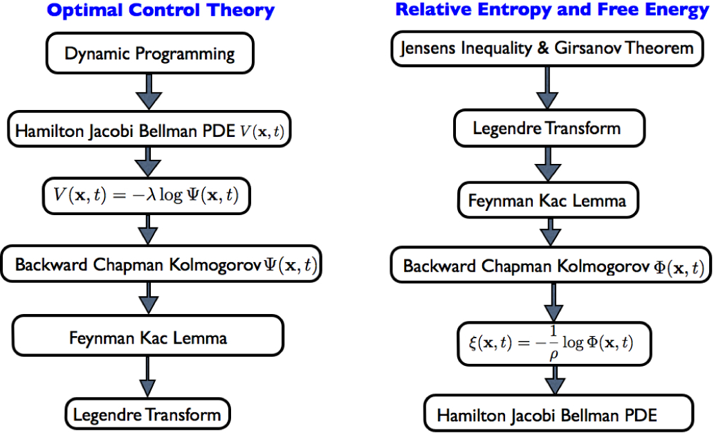
  • The PI and KL control framework can be derived using the relative entropy-free energy relationship, and therefore, there are direct connections of the LSOC framework to previous work in control theory. These connections were recently shown in [11]. From the epistemological stand point, the aforementioned connections provide a deeper understanding of optimality principles and identify the conditions under which these optimality principles emerge from information theoretic postulates. Essentially, there are alternative views/methodological approaches of looking into nonlinear stochastic optimal control that are illustrated in Figure 1.
  • The derivation of nonlinear stochastic optimal control using the free energy and relative entropy relationship does not rely on the Bellman principle. In other words, one can derive the Hamilton–Jacobi–Bellman (HJB) equation without using dynamic programming. When the form of the optimal control policy has to be found, then the connection with stochastic optimal control based on dynamic programming is necessary. In this paper, we generalize the connection between free energy-relative entropy dualities and stochastic optimal control to systems that are non-affine in controls. The analysis leverages the generalized version of the Feynman–Kac lemma and identifies the necessary and sufficient conditions under which the aforementioned connections are valid. This generalization creates future research directions towards the development of optimal control algorithms for stochastic systems nonlinear in the state and control. In addition, it shows that there is a deeper relation between the Legendre transformation and stochastic control that goes beyond the class of control affine systems.
  • While typically in stochastic optimal control theory, the cost function is pre-specified, this is not the case when the stochastic optimal control framework is derived using the free energy-relative entropy relationship. In the latter case, the form of the cost function related to control effort emerges from the structure of the underlying stochastic dynamics. This observation indicates that there are strong interdependencies between cost functions and dynamics and that the choice of the control cost function is not arbitrary. Another way to understand the importance of the aforementioned interdependencies is that, while in the traditional approach, the cost function is imposed to the problem, in the information theoretic view of stochastic optimal control, the cost function partially emerges from the formulation of the problem (see Figure 1).
  • We illustrate connections between stochastic control and the maximum entropy principle. The analysis relies on the generalized Boltzmann, Gibbs and Shannon entropy [16]. We show that the stochastic control framework is recovered as the maximization of the generalized Boltzmann, Gibbs and Shannon entropy subject to energy and probability measure normalization constraints.
  • For the class of stochastic systems that are affine in control and noise, there are cost function formulations that cannot be represented within the information theoretic approach. Thus, although the information theoretic formulation of stochastic optimal control provides a general framework, there are cases in which the a priori specification of the cost function and the use of dynamic programming provide more flexibility.
  • Besides the analysis on the connections between different formulations of stochastic optimal control theory, we also present iterative algorithms designed for stochastic systems and demonstrate some examples.
The paper is organized as follows. In Section 2, we provide the definitions of free energy and relative entropy and derive their mathematical connection. In Section 3 we present the connection of the relative entropy and free energy relationship with the theory of stochastic control. In particular, in Section 3.1, we apply the relative entropy and free energy relationship to nonlinear stochastic dynamical systems affine in noise. In Section 3.2, the analysis on the application of the aforementioned relationship to nonlinear stochastic dynamics affine in controls and noise is presented together with connections to dynamic programming. In Section 4, we discuss thermodynamic interpretations and connections to the maximum entropy principle. In Section 5, we provide the derivation of the PI control as presented within the machine learning and statistical physics. In Section 6, the discrete time formulation is derived, and in Subsection 6.1, the connections to continuous time are shown. Finally in Section 7, we present algorithms, and in Section 8, we conclude with a discussion on the equivalencies and differences between the different views of stochastic optimal control.

2. Fundamental Relationship between Free Energy and Relative Entropy

In this section, we discuss the fundamental relationship between free energy and relative entropy [13]. This relationship is key for deriving the stochastic optimal control problem. Let (Ω, ) be a measurable space, where Ω denotes the sample space and denotes a σ-algebra, and let P (Ω) define a probability measure on the σ-algebra . For the concepts that we shall propose, we need the following definitions.
Definition 1. Let ℙ ∈ P (Ω), and let the function (x): Ω → ℜ be a measurable function. Then, the following term:
E = log e exp ( ρ J ( x ) ) d P ,
is called the free energy (the function loge denotes the natural logarithm) of J (x) with respect to ℙ and ρ ∈ ℜ.
Definition 2. [13]: Let ℙ ∈ P (Ω) and ℚ ∈ P (Ω); then, the relative entropy of ℙ with respect to ℚ is defined as:
K L ( Q P ) = { + , otherwise , log e d Q d P d Q , if Q < < P and log e d Q d P 1 ,
where “≪” denotes the absolute continuity of ℚ with respect to ℙ and 1 denotes the space of Lebesgue measurable functions on [0, ∞). We say that ℚ is absolutely continuous with respect to ℙ, and we write ℚ ≪ ℙ if ℙ(H) = 0 ⇒ ℚ(H) = 0, ∀H.
The free energy and relative entropy relationship is expressed by the theorem that follows.
Theorem 1. Let (Ω, ) be a measurable space, wheredenotes the sample space and denotes a σ-algebra, and let P(Ω) define a probability measure on the σ-algebra . Consider ℙ, ℚ ∈ P(Ω) and the definitions of free energy and relative entropy as expressed in Definitions (1) and (2). Under the assumption that ℚ ≪ ℙ, the following inequality holds:
1 | ρ | log e E P [ exp ( | ρ | J ) ] [ E Q ( J ) + | ρ | 1 K L ( Q | | P ) ] ,
where E P, E Q is the expectation under the probability measure ℙ, ℚ, respectively, and ρ ∈ ℜ and : ℜM → ℜ and M Z +. The inequality in (2) is the so-called Legendre transform.
Proof. We express the expectation E P as a function of the expectation E Q. In particular,
E P [ exp ( ρ J ) ] = exp ( ρ J ) d P = exp ( ρ J ) d P d Q d Q .
Taking the logarithm of both sides of Equation (3) and using Jensen’s inequality yields:
log e E P [ exp ( ρ J ) ] = log e exp ( ρ J ) d P d Q d Q log e ( exp ( ρ J ) d P d Q ) d Q
The inequality (4) can be written as:
log e E P [ exp ( ρ J ( x , t ) ) ] ( ρ J + log d P d Q ) d Q = ρ J d Q K L ( Q | | P ) .
Multiplying Equation (5) with 1 ρ, where ρ < 0 or ρ = −|ρ|, it follows Equation (2) with E Q ( J ) = J d Q.
Inequality (2) gives a dual relationship between relative entropy and free energy, which leads to the minimization problem:
1 | ρ | log e E P [ exp ( | ρ | J ) ] = inf d Q [ E Q ( J ) + | ρ | 1 K L ( Q | | P ) ] ,
The infimum in Equation (6) attained at ℚ* is given by:
d Q * = exp ( | ρ | J ) d P exp ( | ρ | J ) d P .
To verify that the infimum is attained by Equation (2), we have the following lemma.
Lemma 1. Given the definitions of free energy and relative entropy and the assumption of absolutely continuous measures ℚ ≪ ℙ, the LHS of the Legendre transformation in Equation (2) is attained by the optimal measure in Equation (7).
Proof. The proof is rather, simple and it is based on the substitution of Equation (7) into Equation (2). More precisely:
E Q * [ J ] + 1 | ρ | K L ( Q * | | P ) = E Q * [ J ] + 1 | ρ | log e d Q * d P d Q * = E Q * [ J ] + 1 | ρ | log e exp ( | ρ | J ) d P exp ( | ρ | J ) d P d P d Q * = E Q * [ J ] + 1 | ρ | log e exp ( | ρ | J ) exp ( | ρ | J ) d P d Q * = E Q * [ J ] + 1 | ρ | [ | ρ | J ( x ) ) ] d Q * 1 | ρ | log e exp ( | ρ | J ) d P ] d Q * = 1 | ρ | [ log e exp ( | ρ | J ) d P ] d Q * = 1 | ρ | log e exp ( | ρ | J ) d P d Q * = 1 | ρ | log e exp ( | ρ | J ) d P
In the case where ρ > 0, the inequality in (2) is flipped, and hence, the infimum in Equation (6) reverts to a supremum.

3. The Legendre Transformation and Stochastic Optimal Control

With the goal to use the Legendre transformation and to show its connection to optimal control, we define as a state- and time-dependent cost function evaluated on trajectories starting at x(t) ∈ ℜn at time t and with a time horizon tNt. More precisely, we have the mathematical form:
J = J ( x ( ) , t ) = ϕ ( x ( t N ) , t N ) + t t N q ( x , τ ) d τ .
where ϕ: ℜn × ℜ → ℜ is a state-dependent terminal cost and q: ℜn × ℜ → ℜ is state- and time-dependent running cost. We also define the function ξ: ℜn × ℜ → ℜ as follows:
ξ ( x , t ) = 1 ν log e E P [ exp ( ν J ( x , t ) ) ] ,
where v ∈ ℜ. Depending on the sign of ν, the function ξ(x; t) has different interpretations. For small ν, Equation (9) is a function of the mean and the variance ξ ( x , t ) = E P ( J ( x , t ) ) + ν 2 VA ( J ( x , t ) ). For ν = |ρ|, Equation (9) is risk sensitive, whereas for ν = −|ρ|, it is risk seeking. For our analysis, ν = −|ρ|. Next, we incorporate the state and time dependencies in the Legendre transformation in Equation (6), and we have:
ξ ( x , t ) = 1 | ρ | log e E P [ exp ( | ρ | J ( x , t ) ) ] Desirability Helmholtz Free Energy = inf d Q [ E Q ( J ( x , t ) ) State Cost + | ρ | 1 K L ( Q | | P ) Information Cost ] .
The RHS of the minimization problem in Equation (10) is the sum of a state-dependent cost and the relative entropy between the two measures ℙ, ℚ; moreover, the minimization is w.r.t the probability measures ℚ. We assign the probability measures ℙ and ℚ to passive, in the sense of uncontrolled dynamics, and to controlled dynamics and consider the task of steering a dynamical system from an initial to a target state. The goal in Equation (10) is to find the optimal probability measure/control that steers the system from the initial to the terminal state by minimizing the state cost at the expense of the information cost. The information cost is an implicit measure of control effort, and its final formulation depends on the structure of the underlying dynamics. The LHS in Equation (10) corresponds to Helmholtz free energy, while there is also a term that corresponds to the concept of the desirability function. This concept was introduced in [4] and plays a key role in our derivations and analysis that follow. In the next two sections, we apply the Legendre transformation to stochastic systems and identify the cases where there is a direct relationship with dynamic programming and the LSOC.

3.1. Application to Nonlinear Stochastic Dynamics with Affine Stochastic Disturbances

In this section, we consider stochastic dynamics of the form:
d x = F ( x , u ) d t + B ( x ) d w ( 1 ) , x ( 0 ) = x 0 , t 0 ,
where x ∈ ℜn denotes the state of the system, u ∈ ℜm denotes the control vector, B(x): ℜn → ℜn×p is the diffusion matrix function, F(x, u): ℜn × ℜm → ℜn are the drift dynamics and dw ∈ ℜp is a Gaussian white noise disturbance. The diffusion matrix is partitioned as B ( x ) = [ 0 ( n p ) × p T , B c T ( x ) ] T where Bc(x): ℜn → ℜp×p is invertible and B c ( x ) = B ( x ) B T ( x ) : n p × p. Similarly, the drift term is partitioned as F ( x , u ) = [ F m T ( x , u ) , F c T ( x , u ) ] T, where Fm(x, u): ℜn × ℜm → ℜ(np) and Fc(x, u): ℜn × ℜm → ℜp. Next, define the stochastic differential equation:
d x = A ( x ) d t + B ( x ) d w ( 0 ) , x ( 0 ) = x 0 , t 0 ,
where the drift term A(x): ℜn → ℜn is defined as A(x) ≜ F(x, 0)and corresponds to the uncontrolled dynamics in Equation (11). Here, we denote the expectations evaluated on the system trajectories generated by the controlled dynamics and uncontrolled dynamics by E Q and E P, respectively. In addition, ΔFm(x, u) ≜ Fc(x, u) − Ac(x) = Fc(x, u) − Fc(x, 0). The definition of the Radon–Nikodym [17] derivative for the stochastic differential Equations (11) and (12) has the form:
d Q d P = exp ( ζ ( u , t ) ) ,
where the term ζ(u, t) is now defined as:
ζ ( u , t ) = t t N Δ F c T ( x , u ) B c ( x ) 1 ( x ) d w ( 1 ) d τ + t t N 1 2 Δ F c T ( x , u ) B c 1 ( x ) Δ F c ( x , u ) d τ .
Now, substituting Equations (13) and (14) into Equation (2), we obtain:
ξ ( x , t ) E Q [ J ( x , t ) ] State Cost + E Q [ 1 2 | ρ | t t N Δ F c T ( x , u ) B c 1 ( x ) Δ F c ( x , u ) d τ ] Information Cost .
When the minimum is attained for ℚ* given by Equation (7), we have:
ξ ( x , t ) = E Q * [ ϕ ( x ( t N ) , t N ) + t t N q ( x , τ ) d τ + 1 2 | ρ | t t N Δ F c T ( x , u * ) B c 1 ( x ) Δ F c ( x , u * ) d τ ] ,
where the ΔFc(x, u) ≜ Fc(x, u) − Fc(x, 0) corresponds to the difference between the drift of the optimally-controlled (i.e., u = u) and the drift of the uncontrolled (i.e., u = 0) dynamics. Equations (15) and (16) demonstrate how the structure of the dynamics appears in the information cost under minimization in the Legendre transformation. Therefore, there is a straight-forward relationship between the structure of the stochastic dynamics under consideration and the form of the control cost function under minimization. While this observation is not surprising when the Legendre transformation is used, it suggests ways to design control cost functions in stochastic optimal control theory based on the form of the stochastic dynamics. Another interesting observation is that the LHS of Equation (16) is the minimum attained under the optimal, in the sense of the Legendre transformation, probability measure ℚ.
A question that arises here is related to the connection between the two forms of optimality, namely the optimality in the Legendre sense and the optimality in the dynamic programming sense. To further investigate this connection, we will leverage the Feynman–Kac Lemma in its more general form for the case of backward PDEs [8]. We also consider the stochastic dynamics in Equation (11) under the optimal control law u(x, t):
dx = F ( x , u * ( x , t ) ) d t + B ( x ) d w ( 1 ) , x ( 0 ) = x 0 , t 0 ,
Under the assumptions of continuity and linear growth for F(x, u(x, t)), B(x) and the existence and uniqueness of the weak solution of Equation (17) (see pages 364 and 366 of [8]), we have the following theorem:
Theorem 2. Feynman–Kac: Let Ψ(x, t): [0, tN] × ℜn → ℜ be continuous and Ψ(x, t) ∈ C1,2, and it satisfies the Cauchy problem:
t Ψ = 1 λ Ψ + F T ( x Ψ ) + 1 2 tr ( ( xx Ψ ) BB T ) + ( x , t )
in [0, tN) × ℜ1 with the boundary condition:
Ψ ( x , t N ) = β ( x )
then Ψ(x, t) admits the stochastic representation:
Ψ ( x , t ) = E [ β ( x t N ) exp ( 1 λ t t N ( x s , τ ) d τ ) + t t N ( x , t ) exp ( 1 λ t s ( x s , τ ) d τ ) d s ]
t0 ∈ [0, tN]. In particular, such a solution is unique. The expectation above is taken with respect to sampled trajectories generated using (17).
Given the form of the Feynman–Kac lemma and the expectation in Equation (16), we set the terms (x, t), ℓ and β ( x t N ) in Equation (20) as follows:
( x , t ) = q ( x ) + 1 2 | ρ | Δ F c T ( x , u * ) B c 1 ( x ) Δ F c ( x , u * ) d τ , ( x , t ) = 0 , β ( x t N ) = ϕ ( x ( t N ) t N )
Based on the Feynman–Kac lemma, the free energy term ξ(x, t) can be interpreted as the unique solution of the backward PDE:
ξ ( x , t ) t = q ( x , t ) S t a t e C o s t + 1 2 | ρ | Δ F c T ( x , u * ) B c 1 ( x ) Δ F c ( x , u * ) Optimal Control Cost + ξ x T ( x , t ) F ( x , u * )
with the boundary condition ξ(x(tN), tN) = ϕ(x(tN), tN). The interesting observation here is that the PDE in Equation (22) is the optimal HJB PDE for a stochastic optimal control problem with state cost q(x, t) and control cost term 1 2 | ρ | Δ F c T ( x , u * ) B c 1 ( x ) Δ F c ( x , u * ) subject to the dynamics in Equation (11). It is clear therefore that there is a fundamental connection between the Legendre transformation and dynamic programing for the general class of stochastic systems that are affine only in the stochastic disturbances and nonlinear in controls and states. This observation generalizes our previous work on identifying the connections between the relative entropy and free energy dualities and the PI and KL controls [11]. Essentially, the two methodologies result in the same HJB PDE when the state and the control cost function are defined as:
State Cost = q ( x , t ) , Control Cost = 1 2 | ρ | Δ F c T ( x , u ) B c 1 ( x ) Δ F c ( x , u )
The implications of this finding can be summarized as follows
  • The Helmholtz free energy satisfies the HJB PDE for the case of systems that are non-affine in controls and affine in stochastic disturbances. This observation has direct consequences to the development of algorithms that can compute the value function for a stochastic optimal control problem with forward sampling of SDEs. While this connection was known within the LSOC framework for dynamics affine in controls and noise, it is the first time that this connection has been derived for general classes of stochastic systems with dynamics nonlinear in state and control and affine only in noise.
  • The optimal measure dℚ for the stochastic control problem with state and control cost as specified in Equation (23) is given by Equation (7). Note that this is the probability measure that corresponds to trajectories generated under the optimal control policy u(x, t). A fundamental question at this point is related to how this optimal control can be numerically computed, such that dℚ = dℚ. The difficulty arises from the fact that for the case of dynamic systems that are nonlinear in controls and cost functions that are non quadratic, there is no explicit form for the optimal control policy u(x, t). This difficulty could be addressed by an a priori specification of the structure of the optimal control policy u(x, t) and then optimization of this structure, such that for any state x and time t, the optimal probability measure dℚ = dℚ(x, t) is reached.
Next, we discuss the connection between the free energy-relative entropy dualities and stochastic optimal control of systems with dynamics affine in control and noise. Again, the Feynman–Kac lemma plays a key role, but as will be shown, the way that it is applied differs from our analysis in this section, since it is directly applied to the desirability function.

3.2. Application to Nonlinear Stochastic Dynamics with Affine Controls and Disturbances

In this section, we apply the Legendre transformation for probability measures that correspond to stochastic dynamics affine in control and stochastic disturbances. In particular, we consider the stochastic dynamics [13,18]:
d x = f ( x ) d t + 1 | ρ | ( x ) d w ( 0 ) , x ( 0 ) = x 0 , t 0 ,
d x = f ( x ) d t + ( x ) ( u d t + 1 | ρ | d w ( 1 ) ) , x ( 0 ) = x 0 , t 0
where x ∈ ℜn denotes the state of the system, (x): ℜ → ℜn×p is the control and diffusion matrix function partitioned as ( x ) = [ 0 ( n p ) × p T , c T ( x ) ] T, where c(x): ℜ → ℜp×p is invertible, f(x): ℜn → ℜ denotes the passive dynamics, u ∈ ℜp is the control vector and dw ∈ ℜp is a Gaussian white noise disturbance. Note that the difference between the two diffusion terms in Equations (24) and (25) is the fact that the control appears in Equation (25). This control, together with the passive dynamics, defines a new drift term. Expectations evaluated on the system trajectories generated by the uncontrolled and controlled dynamics are represented by E and E, respectively. The corresponding probability measures of the aforementioned expectations are ℙ and ℚ. Next, we use Equation (10) and the Radon–Nikodym derivative given by Equations (13) and (14), which now takes the form d Q d P = exp ( ζ ( u , t ) ) [8], where the term ζ (u, t) is given by:
ζ ( u , t ) = 1 2 | ρ | t t N u T u d τ + | ρ | t t N u T d w ( 1 ) ,
Substitution d Q d P into inequality (10) gives:
ξ ( x , t ) = 1 | ρ | log e E P [ exp ( | ρ | J ( x , t ) ) ] E Q [ J ( x , t ) + 1 | ρ | ζ ( u , t ) ]
Substitution of ζ (u) in the last equation results in:
ξ ( x , t ) = 1 | ρ | log e E P [ exp ( | ρ | J ( x , t ) ) ] E Q [ J ( x , t ) + 1 2 t t N u T u d τ ] .
The last term in Inequality (28) corresponds to the cost function of a stochastic optimal control problem and is bounded from below by the free energy. In addition to providing a lower-bound on the objective function for the stochastic optimal control problem, Inequality (28) provides an explicit construction on how this lower bound can be computed. This computation involves forward sampling of the uncontrolled dynamics, evaluation of the expectation of the exponentiated state-dependent part, ϕ(x(tN)) and q(x(t)), and the logarithmic transformation of this expectation. Note that Inequality (28) is derived without relying on any principle of optimality and involves the application of Girsanov’s theorem between controlled and uncontrolled stochastic dynamics, as well as the use of the dual relationship between the free energy and the relative entropy needed to compute the lower bound in (28). Inequality (28) defines a minimization problem where the RHS of the inequality is minimized with respect ζ (u, t) and, hence, with respect to the control u. At the minimum u = u, the right part of the inequality in (28) attains its optimal ξ(x, t). Under the optimal control policy u, the optimal distribution takes the from:
d Q * ( x , t ) = exp [ | ρ | ( ϕ ( x ( t N ) ) + t t N q ( x , τ ) d τ ) ] d P exp [ | ρ | ( ϕ ( x ( t N ) ) + t t N q ( x , τ ) d τ ) ] d P .
An important question that arises is: What is the link between (28) and the principle of optimality in dynamic programming? To address this question, one needs to show that ξ(x, t) satisfies the HJB equation, and hence, ξ(x, t) is the corresponding value function [18]. More precisely, we introduce a new variable Φ(x, t) defined as Φ(x, t) ≜ E P (exp (ρ (x, t))) and apply the Feynman–Kac lemma [7] to arrive at the backward Chapman–Kolmogorov PDE:
t Φ ( x , t ) = | ρ | q ( x , t ) Φ ( x , t ) + f T ( x ) Φ x ( x , t ) + 1 2 | ρ | tr ( Φ xx ( x , t ) ( x ) T ( x ) ) .
Since ξ ( x , t ) = 1 ρ log Φ ( x , t ) = 1 | ρ | log Φ ( x , t ), it follows that tΦ(x, t) = −|ρ|Φ(x, t)t ξ(x, t), Φx(x, t) = − |ρ|Φ(x, t)ξx and Φ xx ( x , t ) = | ρ | Φ ( x , t ) ξ xx ( x , t ) | ρ | 2 Φ ( x , t ) ξ x ( x , t ) ξ x T ( x , t ). In this case, it can be shown that ξ(x, t) satisfies the nonlinear PDE:
t ξ ( x , t ) = q ( x , t ) + ξ x T ( x , t ) f ( x ) 1 2 ξ x T ( x , t ) ( x ) T ( x ) ξ x ( x , t ) + 1 2 | ρ | tr ( ξ xx ( x , t ) ( x ) T ( x ) ) .
The nonlinear PDE in Equation (31) corresponds to the HJB equation [19] for the case of the minimizing optimal control problem, and hence, ξ(x, t) is the corresponding minimizing value function. It is important to note that the principle of optimality was not used to derive Equation (31). Furthermore, while the mathematical analysis results in the HJB PDE, it does not explicitly provide the form of the optimal control policy. This means that to derive Equation (31), it is not required to have an expression for the optimal control policy. This observation is in stark contrast with the classical treatment of stochastic optimal control theory, based on dynamic programming, where first the optimal control is specified and then the final form of the HJB Equation (31) is derived.
The optimal control policy associated with Equation (31) is expressed as:
u ( x , t ) = T ( x ) ξ x ( x , t ) .
To recover the optimal control policy Equation (32), one needs to be aware of the optimal control derivation that is based on dynamic programming.

4. Thermodynamic Interpretations and Connections to the Maximum Entropy Principle

In this section, we discuss thermodynamic interpretations of nonlinear stochastic optimal control theory using the relative entropy-free energy relationship. More precisely, we consider the Baroh–Jaunch entropy or generalized Boltzmann–Gibbs–Shannon entropy [16] defined as:
S ( Q | | P ) K L ( Q | | P ) = d Q d P log e d Q d P d P ,
then Equation (2) takes the form:
1 | ρ | log e E P [ exp ( | ρ | J ( x , t ) ) ] F : Helmholtz Free Energy = inf d Q [ E P ( J ( x , t ) ) U : State Cost T S ( Q | | P ) S : Generalized Entropy ] .
At ℚ = ℚ, we have that:
1 | ρ | log e E P [ exp ( | ρ | J ( x , t ) ) ] F : Helmholtz Free Energy = E Q * ( J ( x , t ) ) U : State Cost T S ( Q | | P ) S : Generalized Entropy ,
The last equation has the form F = UT S, where F is the free energy, T = |ρ|1 is the temperature and S is the generalized Boltzmann–Gibbs–Shannon entropy. Note that Baroh–Jaunch entropy is a concave function, and it is a generalized form of entropy, since it incorporates the Boltzmann, Gibbs and Shannon entropy [16]. In addition, it is negative, and its maximum is reached for ℙ = ℚ. Minimization of the K L ( P | | Q ) is equivalent to maximization of the generalized Boltzmann–Gibbs–Shannon entropy S ( P | | Q ). In the absence of the state cost, the optimal measure is the one that maximizes the Boltzmann–Gibbs–Shannon entropy, and therefore, ℙ = ℚ. However, as it is shown next, in the presence of the state-dependent cost constraint, the optimal measure ℚ should be “far” from the baseline probability measure ℙ. When the probability measures ℚ and ℙ are assigned to state distributions of controlled and uncontrolled stochastic dynamical systems, the Kullback–Leibler divergence between ℚ and ℙ is an implicit measure of control effort. In this sense, minimization of the Kullback–Leibler divergence or maximization of the generalized Boltzmann–Gibbs–Shannon entropy is equivalent to minimization of the control effort.
Another interesting connection with thermodynamics emerges from the fact that the optimal policy can be derived using the maximum entropy principle. The form of entropy under maximization is the generalized Boltzmann–Gibbs–Shannon entropy. To makes things concrete, lets consider the following maximum entropy constrained optimization problem specified as follows:
max d Q * S ( Q | | P ) Subject to : E Q [ J ( x , t ) ] = c and d Q = 1 .
where c is positive constant. To find the solution, we form the augmented objective function by incorporating the constraints with proper Lagrange multipliers:
( Q , λ , μ , c ) = S ( Q | | P ) + λ ( c E Q [ J ( x , t ) ] ) + μ ( 1 d Q ) = d Q d P log e d Q d P d P + λ ( c J ( x , t ) d Q ) + μ ( 1 d Q ) = ( log e d Q d P + λ J ( x , t ) + μ ) d Q + λ c + μ .
Next, we define the term:
L = ( log e d Q d P + λ J ( x , t ) + μ ) f d Q
Given the assumptions that f is ℚ-integrable and the signed measure L is absolute continuous with respect to ℚ, ( L≪ ℚ), the signed measure L is finite (see the general form of Radon–Nikodym Theorem 5.5.3 in [20]). Later, it will be shown that L is a measure (positive-signed measure), but for now, we consider the more general case of the signed measure. Under the aforementioned assumptions, the Radon–Nikodym derivative d ( Q ) d Q is a well-defined operation. To find the optimal measure ℚ, we apply the Radon–Nikodym derivative in Equation (38) and set it to zero. In mathematical terms, this operation results in:
log e d Q * d P + λ J ( x , t ) + μ = 0 d Q * = exp ( λ J ( x , t ) μ ) d P .
Integration of the optimal measure dℚ to one gives an expression for µ:
μ = log e exp ( λ J ( x , t ) ) d P .
Substitution of µ back in Equation (39) gives the optimal probability measure in Equation (7). There are few interesting observations:
  • Substitution of the optimal measure dℚ in Lagrangian (37) results in:
    ( Q * , λ , μ , c ) = λ c + log e exp ( λ J ( x , t ) ) d P
    Moreover, given a certain performance level c, the Lagrange multiplier λ can be found by using the equation:
    J ( x , t ) d Q * c = 0 ( J ( x , t ) c ) exp ( λ J ( x , t ) d P = 0 ) .
  • The term 1 λ μ = 1 λ μ ( x , t ) corresponds to the Helmholtz free energy, since:
    1 λ μ ( x , t ) = 1 λ log e exp ( λ J ( x , t ) ) d P .
    Therefore, for the case stochastic dynamics affine in control and noise, the term 1 λ μ function and satisfies the HJB equation.
  • Initially, we considered L as a singed measure. However, given the optimal measure ℚ and the form of the Lagrange multiplier µ, the signed measure L is positive, and therefore, it is a measure. To show this, one can use the Legendre transformation between free energy and relative entropy.
The thermodynamic equilibrium of maximum entropy corresponds to maximization of the generalized Boltzmann–Gibbs–Shannon entropy that is equivalent to minimization of control effort subject to the performance and normalization constrains as expressed in the optimization problem in Equation (36). Moreover, the equilibrium measure is the optimal measure as specified in Equation (7). For the case of stochastic dynamics affine in controls and noise, this measure corresponds to trajectories sampled from the stochastic dynamics under the optimal, in the sense of dynamic programming, control policy.

5. Bellman Principle of Optimality

In this section, we consider the classical stochastic optimal control problem as a constrained optimization problem and derive the LSOC framework in continuous time. The analysis in this section is more known under the name of PI control, and it has been presented mostly in the machine learning and statistical physics communities [2,21].
Here, we present a generalized version, which was also derived in [11], which allows terms in the cost function to be both state and control dependent. This formulation is important for our later discussion on the generalizability of every approach (information theoretic, path integral, KL control) in the LSOC framework. In particular, we start with the cost functional:
V ( x , ( t ) , t ) = min u J ( x , u ) = min u E Q [ ϕ ( x , t N ) + t t N ( x , u , τ ) d τ ] .
The expectation E in Equation (42) is evaluated on system trajectories generated by forward sampling of the controlled diffusion process Equation (11). We assume that the function F(x, u) is a nonlinear function of the state x ∈ ℜn and affine in the control u ∈ ℜm, and hence, F(x, u) = f(x) + G(x)u. The matrix function G(x): ℜn → ℜn×m is the control transition matrix, and f(x): ℜn → ℜn denotes the passive dynamics. Under the optimal control u = u, the cost function J(x, u) is equal to the value function V (x, t). Next, let (x, u, t) denote the running cost defined as L(x, ( x , u , t ) q 0 ( x , t ) + q 1 T ( x , t ) u + 1 2 u T Ru, where q0(x, t) is a nonlinear, nonquadratic state-dependent cost, q 1 T ( x , t ) u is a cross-term depending on the state and control and 1 2 u T Ru is a quadratic control cost with R > 0. The stochastic HJB equation [15,19] associated with this stochastic optimal control problem can be expressed as follows:
t V ( x , t ) = min u ( ( x , u , t ) + V x T ( x , t ) F ( x , u ) + 1 2 tr ( V xx ( x , t ) B ( x ) B T ( x ) ) ) .
The corresponding optimal control is given by:
u ( x , t ) = R 1 ( q 1 ( x , t ) + G T ( x ) V x ( x , t ) ) .
The optimal control drives the system dynamics in the direction opposite that of the gradient of the value function Vx(x, t). Furthermore, the value function satisfies the nonlinear, second-order PDE:
t V ( x , t ) = q ˜ ( x , t ) + V x T ( x , t ) f ˜ ( x , t ) 1 2 V x T ( x , t ) G ( x ) R 1 G T ( x ) V x ( x , t ) + 1 2 tr ( V xx ( x , t ) B ( x ) B T ( x ) ) ,
where q ˜ ( x , t ) q 0 ( x , t ) 1 2 q 1 ( x , t ) T R 1 q 1 ( x , t ) and f ˜ ( x , t ) f ( x ) G ( x ) R 1 q 1 ( x , t ), and the boundary condition V (x(tN); tN) = ϕ(x(tN); tN) Given the exponential transformation and the relationship between control authority and noise:
V ( x , t ) = λ log ψ ( x , t ) , λ G ( x ) R 1 G T ( x ) = B ( x ) B T ( x ) = ( x ) ,
the PDE in Equation (45) yields:
t ψ ( x , t ) = 1 λ q ˜ ( x , t ) ψ ( x , t ) + f ˜ T ( x ) ψ x ( x , t ) + 1 2 tr ( ψ xx ( x , t ) ( x , t ) ) ,
with boundary condition ψ = exp ( 1 λ ϕ ( x , t N ) ). Now, applying the Feynman–Kac lemma to the Chapman–Kolmogorov PDE Equation (47) yields a solution in the form of an expectation over system trajectories; namely:
ψ ( x , ( t ) , t ) = E P ˜ [ exp ( t t N 1 λ q ˜ ( x , τ ) d τ ) ψ ( x ( t N ) t N ) ] .
The expectation E P ˜ in Equation (48) is taken on sample paths generated with the forward sampling of the uncontrolled diffusion equation d x = f ˜ ( x ) d t + B ( x ) d w, and the optimal control is given by:
u ( x ( t ) , t ) = R 1 ( q 1 ( x , t ) λ G T ( x ) ψ x ( x , t ) ψ ( x , t ) ) .
Since the initial value function V (x, t) is the minimum of the expectation of the objective function J(x, u) subject to controlled stochastic dynamics, it can be shown that:
V ( x , t ) = λ log e E P [ exp ( t t N 1 λ q ˜ ( x , t ) d τ ) ψ ( x ( t N ) , t N ) ] Helmholtz Free Energy E Q [ J ( x , u ) ] Total Cost .
Note that Equation (50) is a form of the Legendre transformation, and in fact, it is identical to Equation (28) for the case where q 1 ( x , t ) = 0 , R = I , λ = 1 | ρ | , G ( x ) = ( x ) and ( x ) = 1 | ρ | ( x ). With the derivation of the PI stochastic control starting with dynamic programming in continuous time, it is obvious that the mathematical steps follow the opposite direction as in the section where the the same framework is derived based on the relative entropy-free energy dualities; see Figure 1. Furthermore, within the class of stochastic systems affine in controls and stochastic disturbances, the approach that is discussed in this section provides more general formulations, since it allows cost functions with terms that are both state and control dependent, such as the term q 1 T ( x , t ) u. These terms cannot be recovered when the information theoretic approach is used for the class of stochastic systems with affine controls and disturbances. Therefore, under these certain conditions, the dynamic programming approach provides more flexibility in designing cost functions for optimal control problems.

6. Kullback–Leibler Control in Discrete Formulations

The KL control was presented in its most generalized form in [4]. In this section, we will review the KL control for the finite horizon case. A preliminary analysis on the information theoretic connection of the KL control for the infinite horizon case can be found in [6]. Within the KL control framework, the stochastic optimal control problem is formalized as a Markov decision process (MDP) with a stage-wise cost described as:
( x , u ) = q ( x ) + K L ( U ( | x ) P ( | x ) ) = q ( x ) + E x u ( | x ) [ log ( U ( x | x ) P ( x | x ) ) ] .
The KL divergence in the last expression is applied to the one step ahead transition probabilities of the control U ( x | x ) and uncontrolled dynamics P ( x | x ). Application of the Bellman principle of optimality in the finite horizon case results in:
V ( x , t k ) = min P ( | x ) ( q ( x ) + E x U ( | x ) [ log ( U ( x | x ) P ( x | x ) ) + V ( x , t k + 1 ) ] ) ,
where V (x, tk) is the time-varying cost-to-go function. The U ( | x )-dependent terms in the functional above are minimized, and thus, we will have that:
E x U ( | x ) [ log ( U ( x | x ) P ( x | x ) ) + V ( x , t k + 1 ) ] = E x U ( | x ) [ log ( U ( x | x ) P ( x | x ) ) + log ( 1 exp ( V x , t k + 1 ) ) ] = E x U ( | x ) [ log ( U ( x | x ) P ( x | x ) exp ( V x , t k + 1 ) ) ] .
For these purposes, the normalization term G t k [ Φ ] ( x ) is introduced with Φ(x, tk) = exp (−V (x, tk)) being the desirability function. More precisely, we will have:
G t k [ Φ ] ( x ) = x P ( x | x ) Φ ( x , t k + 1 ) = E x P ( | x ) [ Φ ( x , t k + 1 ) ] .
Therefore, we have:
E x U ( | x ) log ( U ( x | x ) P ( x | x ) ) + V ( x , t k + 1 ) = log ( G t k [ Φ ] x ) ) + K L ( U ( | x ) | | P ( x | x ) Φ ( x , t k + 1 ) G t k [ Φ ] ( x ) ) .
Substitution of the expression above into the Bellman minimization equation results in:
V ( x , t k ) = min u U [ q ( x ) log ( G t [ Φ ] ( x ) ) + K L ( U ( | x ) | | P ( x | x ) Φ ( x , t k + 1 ) G t k [ Φ ] ( x ) ) ] .
The minimum of the Bellman equation is attained by:
U * ( x | x ) = P ( x | x ) Φ ( x , t k + 1 ) G t k [ Φ ] ( x ) .
The equation above provides the transition probability under the optimal control law and, in that sense, the optimal transition probability. Substitution of the optimal distribution above will result in the linear Bellman equation:
Φ ( x , t k ) = exp ( q ( x ) ) G t k [ Φ ] ( x ) .
This can be used to prove the path integral representation of the desirability function:
Φ ( x , t k ) = E x τ + 1 P ( | x τ ) [ exp ( τ = t k T q ( x τ ) ) ] .
Thus, the desirability function is just the expectation under the uncontrolled dynamics of the exponentiated path cost starting at state x at time t. This gives an expression for the optimally-controlled trajectory distribution U ( x ) for the trajectory x = { x t i , , x t k , . . x t N } that is specified as follows:
U ( x ) = k = i N U * ( x | x ) = k = i N P ( x | x ) Φ ( x t k + 1 , t k + 1 ) G τ [ Φ ] ( x ) = ( P ( x t k + 1 | x t k ) Φ ( x t k + 1 , t k + 1 ) G τ k [ Φ ] ( x ) ) ( P ( x t k + 2 | x t k + 1 ) Φ ( x t k + 2 , t k + 2 G τ k + 1 [ Φ ] ( x ) ) = ( P ( x t k + 1 | x t k ) exp ( q ( x t k + 1 ) ) G t k + 1 [ Φ ] ( x ) G τ k [ Φ ] ( x ) ) × ( P ( x t k + 2 | x t k + 1 ) exp ( q ( x t k + 2 ) ) G t k + 2 [ Φ ] ( x ) G τ k + 1 [ Φ ] ( x ) ) = ( k i N P ( x t k + 1 | x t k ) ) exp ( J ( x ) ) G τ k [ Φ ] ( x )
Therefore, the optimal trajectory probability has the form:
U ( x ) = P ( x ) exp ( J ( x ) ) E x P ( ) [ exp ( J ( x ) ) ] .
The optimal trajectory probability in the last expression is identical to Equations (7) and (29).

6.1. Connections to Continuous Time
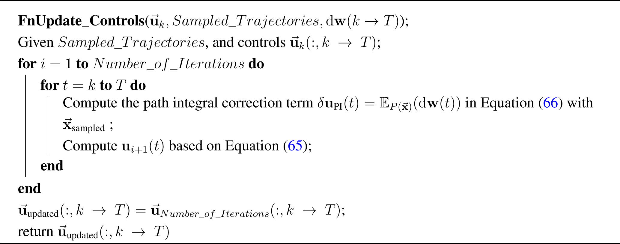
The link of the discrete Bellman Equation in (53) to the corresponding HJB PDE is achieved when expectations E x P ( | x ) and E x U ( ) x are computed using one step ahead states sampled from the uncontrolled and controlled dynamics:
d x = f ( x ) d t + C ( x ) d w d x = f ( x ) d t | + C ( x ) ( u d t + d w )
Due to space limitations, we summarize the derivation of the continuous time LSOC with the following lemma. The derivation can be found in the Supplementary Material of [4].
Lemma 2. Lets consider the dynamics in Equation (56) and the function V(x, t): ℜn × ℜ → ℜ Φ(x, t): ℜn × ℜ → ℜ Φ(x, t) satisfying the linear Bellman equation:
Φ ( d t ) ( x , t k ) = exp ( q ( x ) d t ) G t k [ Φ ( d t ) ] ( x ) .
where q(x) is state-dependent cost and the operator G t k [ Φ ( d t ) ] ( x ) is defined as in Equation (52). If V(x, t) = − loge Φ(x, t), then V(x, t) satisfies the HJB PDE of an optimal control problem.
V ( x ( t 0 ) , t 0 ) = min u E [ t 0 t N ( q ( x ) + 1 2 u T u ) d t ]
subject to controlled dynamics in Equation (56).
This lemma can be seen as an alternative derivation of the Feynman–Kac lemma [9].

7. Algorithms

In this section, we review the derivation of iterative PI control as shown in our previous work [3,11] and also discuss applications and algorithms. In particular, we will start our analysis with the expectation as expressed in Equation (48). Note that this expectation is evaluated over trajectories sampled via forward propagation of uncontrolled diffusion d x = f ˜ ( x ) d t + B ( x ) d w ( 0 ) ( t ) in which f ˜ ( x , t ) = f ( x ) G ( x ) R 1 q 1 ( x , t ). In this paper, we assume that the state of the stochastic dynamics is partitioned as x = [xm xc]T, and the drift and control transition terms are partitioned as follows f ˜ ( x ) = [ f ˜ m T ( x ) f ˜ c T ( x ) ] T G ( x ) = [ 0 ( n m ) × m T G c T ( x m ) ] T, with f ˜ m ( x ) : ( n p ), f ˜ c ( x ) : n p, Gc (xm): ℜp → ℜm×m and diffusion term B ( x ) = [ 0 ( n p ) × p T B c T ( x m ) ] T with Bc(xm): ℜp → ℜp. Note that systems such as multi-body systems have this form. We also assume that:
λ G c ( x m ) R 1 G c T ( x m ) = B c ( x m ) B c T ( x m )
To derive the iterative path integral control, we will start our analysis with the stochastic representation of the solution of backward Chapman–Kolmogorov PDE:
Ψ ( x ( t i ) , t i ) = E P ˜ [ exp ( t i t N 1 λ q ˜ ( x , t ) d t ) Ψ ( x t N ) ] = exp ( t i t N 1 λ q ˜ ( x , t ) d t ) Ψ ( x t N ) d P ˜
Since at every iteration k, the sampling process takes place with the use of the control policy uk(x, t) the expression above is formulated as:
Ψ ( x ( t i ) , t i ) = exp ( t i t N 1 λ q ˜ ( x , , t ) d t ) Ψ ( x t N ) d P ˜ d Q ˜ d Q ˜
where the Q ˜ is the probability measure that corresponds to the diffusion process d x = f ˜ ( x ) d t + G ( x ) u k ( x , t ) d t + B ( x ) d w ( 1 ). The terms uk(x, t) and dw(1) are the control and noise used at iteration k. The ratio of the two probability measures d P ˜ d Q ˜ is the Radon–Nikodým. The aforementioned ratio for stochastic dynamics is formulated as follows:
d P ˜ d Q ˜ = exp [ 1 2 λ t i t N ( u k T ( t ) ϒ uu u k ( t ) δ t ) ] × exp [ 1 λ t i t N ( u k T ( t ) ϒ uw d w ( 1 ) ( t ) ) ]
where the terms ϒuu(x), ϒuw(x) and ϒ are defined as ϒ uu ( x m ) = G c T ( x m ) ϒ 1 G c ( x m ) and ϒ uw ( x m ) = G c T ( x m ) ϒ 1 G c ( x m ) and ϒ = G c ( x m ) R 1 G c T ( x m ) = B c ( x m ) B c T ( x m ). After formulating the probability measure P ˜ and using the equation above, Equation (61) will take the form:
Ψ ( x ( t i ) , t i ) = lim d t 0 1 D ( x i ) exp ( 1 2 λ L k ( x i , u i ( k ) ) ) d x
where L k ( x i , u i ( k ) ) plays the role of the Lagrangian at iteration k that is specified as follows:
L k ( x k ( t i ) , u k ( t i ) ) = ϕ ( x ( t N ) ) + 1 2 j = i N 1 q ˜ ( x ( t j ) , t j ) d t + 1 2 j = i N 1 [ x c ( t j + d t ) x c ( t j ) d t α ( x ( t j ) , u k ( t j ) ) ϒ t j 1 2 ] d t + 1 2 j = i N 1 u k T ( t j ) [ ϒ uu u k ( t j ) + 2 G c T ( x m ( t j ) ) ϒ 1 μ ( x j ) ] d t
where the term α(x(tj), uk(tj) is defined as α (x(tj), ( u k ( t j ) ) = f ˜ c ( x ( t j ) ) G c ( x m ( t j ) ) u k ( t j ) and f ˜ c ( x ( t j ) ) is the drift term defined as f ˜ c ( x ( t j ) ) = f c ( x ( t j ) ) G c ( x ( t j ) ) R 1 q 1 ( x ( t j ) , t j ). The terms u k ( t i ) = { u k ( t i ) , , u k ( t N 1 ) } and x k ( t i ) = { x k ( t i ) , , x k ( t N ) } are the state and control trajectories at iteration k. In addition, the term μ ( x j ) = x c ( t j + d t ) x c ( t j ) d t f c ( x ( t j ) ) G c ( x m ( t j ) ) u k ( t j ), and thus, µ(xj)dt = Bc(xm(tj))dw(1)(t). In a more compact form, Equation (62) can be written as:
Ψ ( x ( t j ) , t i ) = lim d t 0 exp ( 1 2 λ L ˜ k ( x ( t i ) , u k ( t i ) ) ) d x
where L ˜ k = L k + 2 λ log D.
Lemma 3. (Iterative path integral optimal control:) Given the form of the Lagrangian in Equation (63) and the desirability function in Equation (64), the iterative optimal path integral control is specified as:
u k + 1 ( x ( t i ) , t i ) d t = R 1 q 1 ( x ( t i ) , t i ) d t C o s t F u n c t i o n + Ω ( x m ( t i ) ) G c ( x m ( t i ) ) u k ( x ( t i ) , t i ) d t P r e v i o u s C o n t r o l + Ω ( x m ( t i ) ) B c ( x ( t i ) ) δ u P I ( x ( t i ) , t i ) P a t h I n t e g r a l C o n t r o l
The path integral correction term δuPI is given by:
δ u P I ( x ( t i ) , t i ) = E P ( x ) ( d w ( 1 ) ( t i ) | x ( t i ) )
where P ( x ) = e 1 λ L ˜ ( x i ) e 1 λ L ˜ ( x i ) d x i ( c ) while the term (xm(ti)) is defined as:
Ω ( x m ( t i ) ) = R 1 G c T ( x m ( t i ) ) ϒ 1
Proof. The optimal controls based on Relation (49) is specified as:
Ω ( x m ( t i ) ) = R 1 G c T ( x m ( t i ) ) ϒ 1
Proof. The optimal controls based on Relation (49) is specified as:
u ( x ( t ) , t ) = R 1 ( q 1 ( x , t ) λ [ 0 k × p G c T ( x m ) ] ψ x ( x , t ) ψ ( x , t ) ) = R 1 q 1 ( x , t ) + λ R 1 G c T ( x m ) ψ x c ( t ) ( x , t ) ψ ( x , t )
Next, the term ψ x c ( t ) ( x , t ) ψ ( x , t ) is computed where ψ x c ( t ) ( x , t ) = x c ( t ) ψ ( x , t ) In particular, by pushing the gradient inside the expectation in the definition of the desirability function, we have that:
x c ( t ) ψ ( x , t ) ψ ( x , t ) = E P ( x ) ( x c ( t i ) L ˜ ( x i ) )
The term E P ( x ) is the expectation under the probability P ( x ) which is defined as P ( x ) = e 1 λ L ( x i ) e 1 λ L ( x i ) d x i ( c ) Based on the form of the Lagrangian in Equation (63), the term ( x c ( t i ) L ˜ ( x i ) ) takes the form:
( x c ( t i ) L ˜ ( x i ) ) = ϒ 1 ( G c ( x m ( t i ) ) u k ( t i ) + μ ( x t i ) ) + O ( d t )
The notation O ( d t ) is used for terms of order dt. We will keep this notation, as we will see that these terms will cancel. The optimal control is expressed as:
u k + 1 ( x ( t i ) t i ) d t = R 1 q 1 ( x t i , t i ) d t + R 1 G c T ( x m ( t i ) ) E P ( x ) ( x t i ( c ) L ˜ ( x i ) ) d t R 1 q 1 ( x t i , t i ) d t + E P ( x ) ( u L ) + O ( d t 2 )
The term uL in the expression above takes the form:
u L = R 1 G T ( x m ( t i ) ) ϒ ( x m ( t i ) ) 1 ( G c ( x m ( t i ) u k ( t i ) d t + μ ( x t i ) d t )
The multiplication of the optimal controls with dt is done in terms of quadratic order with respect to dt. These terms cancel out as dt → 0 or for very small dt. Finally, since µ(x)dt = B(x)dw(1)(t), we will have that the final result is:
u L = R 1 G T ( x m ( t i ) ) ϒ ( x m ( t i ) ) 1 ( G c ( x m ( t i ) ) u k ( t i ) d t + B c ( x m ( t i ) ) d w ( 1 ) ( t ) )
By combining Equations (69), (68) and (71), the final form for the iterative optimal control is expressed in Equation (67).

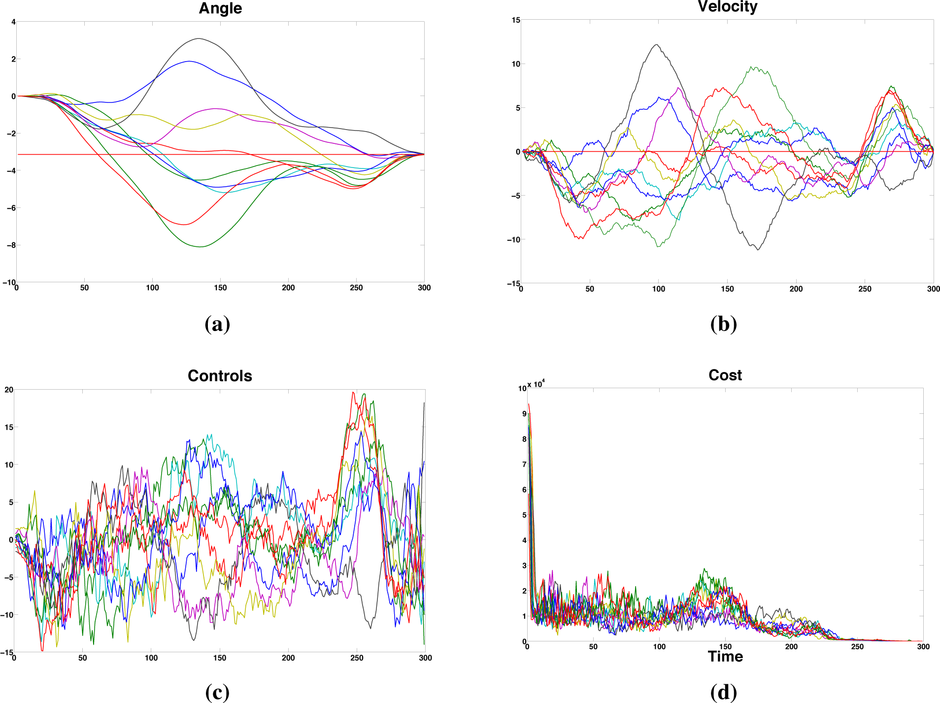
7.1. Open Loop Formulations and Application to an Inverted Pendulum

One of the characteristics of the iterative optimal control in Equation (65) is that the control uk+1(x, t) at iteration k + 1 requires the knowledge of the control uk(x, t) for every pair (x, t). While the iterative characteristic of the proposed scheme improves scalability, the requirement for computing uk(x, t) for any state and time (x, t) prohibits the application of this scheme to high dimensional systems. An alternative approach to address this is to use a parametric or non-parametric approximation method to represent uk(x, t) and apply iterative path integral control in its initial feedback form (65).
Here, we suggest a receding horizon open loop formulation and restrict our analysis to stochastic systems with Bc(x(t)) = Bc, Gc(x) = Gc and q1(x(t), t) = 0. The algorithm is provided in Tables Algorithm 1 and Algorithm 2 and consists of three procedures, namely FnSample_Trajectories, FnUpdate_Controls and FnApply_Control_Dynamics. In particular, the functionality for the procedure FnSample_Trajectories is to sample trajectories starting from state xk by using an initial control trajectory u ( : , k T ) = ( u ( k ) ), u(k + 1), …, u(T)) and to return these sample trajectories and noise profiles used for sampling noise profiles used for sampling dw(:,kT). The next procedure is FnSample_Update and has as input the control trajectory u ( : , k T ), the sampled state trajectories Sampled_Trajectories and the noise profiles dw(:,kT). Its functionality, illustrated in Algorithm 2, is to apply the iterative path integral control in its open loop formulation and to compute the new control trajectory u updated ( : , k T ). In the open loop formulation, the state dependence of the correction term in Equation (66) is dropped, and therefore, the term δuPI(t) becomes only time varying. In FnApply_Control_Dynamics, the control is applied for one time step, and the overall algorithm repeats again.
Algorithm 1:. Iterative stochastic optimal control.
Entropy 17 03352f1
Algorithm 2:. Update_Controls.
Entropy 17 03352f2
Here, we apply the proposed algorithm to a swing up task of an inverted pendulum. The task is to bring the pendulum from initial state x = [x1; x2] = [0; 0] to target state p * = [ p 1 * , p 2 * ] = [ π , 0 ]. The pendulum has mass m = 1 kg and link length l = 0:5 m. The number of sampled trajectories returned by the function FnSample_Trajectories is 200. The terminal cost is ϕ ( x t N , t N ) = 1 , 000 * ( x 1 ( t N ) p 1 * ) 2 + 100 * ( x 2 ( t N ) p 2 * ) 2, and the state cost q(x) = 0 and control cost 1 2 σ 2 u 2. The variance of noise is σ = 0:5, and the time horizon used is tN = 300 * 0:01 = 3 s. The state, control trajectories and the cost are illustrated in Figure 2a–d. In particular, Figure 2a illustrates a set of 10 angular trajectories that reach the desired state(red horizontal line), and Figure 2b illustrates the corresponding angular velocities that also reach the desired state (red horizontal line). Figure 2c illustrates the stochastic iterative path integral control trajectories. Finally, Figure 2d illustrates the cost for the 10 trials as the system moves towards the target state p* under the application of the iterative optimal path integral control.

8. Discussion

In this paper we present four different approaches to LSOC. In the first approach, which is also the most traditional one, stochastic optimal control is formulated as the minimization of an objective function J(x, u) in Equation (42) subject to the controlled dynamics. The HJB PDE is derived based on the Bellman principle of optimality. The exponential transformation of the value function V (x) and the connection between control cost and variance Equation (46) transforms the HJB into the backward Chapman–Kolmogorov. The Feynman–Kac lemma is applied, and the solution of the Chapman–Kolmogorov PDE together with the lower bound on the objective function are provided.
The second approach starts with the risk-seeking version of the cost (x). This quantity has also the form of the Helmholtz free energy. With the application of Girsanov’s theorem between controlled and uncontrolled dynamics and the use of Jensen inequality, the Helmholtz Free energy is the lower bound of the objective function that consists of a state-dependent cost and an information cost, which is a measure of control effort. The link to Bellman optimality is established by showing that the Helmholtz free energy satisfies the HJB equation, and therefore, it is a value function. It should be clear by now that steps to information theoretic representation are in the opposite direction, as shown in Figure 1. While in the information theoretic approach, the analysis starts with the derivation of the Legendre transformation and ends with the HJB PDE, in the traditional approach, the analysis starts from dynamic programming and ends in a special case of the Legendre transformation.
In the third approach, the stochastic optimal control problem is derived using the maximum entropy principle. The optimization problem is formulated as the maximization of the generalized Boltzmann–Gibbs–Shannon entropy subject to performance constraints. The optimization is with respect to a probability measure that corresponds to the controlled dynamics. At the thermodynamic equilibrium, we have the maximization of the generalized Boltzmann–Gibbs–Shannon entropy, which is equivalent to the minimization of the control effort subject to the performance and normalization constrains as expressed in the optimization problem in (29).
In the KL stochastic optimal control framework [4], the treatment is for MDP. The analysis starts with the construction of a cost function that consists of state cost and an information cost defined as the KL divergence between the one step ahead transition probabilities of the control and uncontrolled dynamics. Next dynamic programming is used to derive the Bellman equation in discrete time. The connection to continuous time stochastic optimal control is performed when one step ahead transition probabilities of the control and uncontrolled dynamics correspond to controlled and uncontrolled diffusion processes with the same drift.
In this work, we present different views of nonlinear stochastic control and provide connections, new generalizations and algorithms. Given all of the aforementioned approaches, it is clear that the idea of exponential transformation of the value function existed already in the early work of control theory. However, it was recently conceptualized as desirability and further explored in terms of algorithms, quantum mechanical interpretations and discrete time formulations. While significant progress has been made in both theory and algorithms, there are fundamental assumptions in the frameworks presented in this work that restrict their applicability to systems where the uncertainty is only of a stochastic nature. This means that there are assumptions on the structure of the dynamics that allow uncertainty only due to noise. Given the progress on non-parametric regression methods in statistical machine learning and the different ways to represent uncertainty, future work on stochastic control will focus on the development of theory and algorithms for the stochastic control of systems with unknown and stochastic dynamics. In these cases, uncertainty will not only incorporate stochasticity due to the existence of noise, but it will also include probabilistic representations of the unknown dynamics. Finally, the generalizations and thermodynamic interpretations presented in this work create new research directions towards the development of stochastic control algorithms for general classes of stochastic systems and for information theoretic measures, such as non-extensive entropies that go beyond the entropy measures used in Boltzmann Gibbs statistical mechanics.

Conflicts of Interest

The authors declare no conflict of interest.

References

  1. Kappen, H.J. An introduction to stochastic control theory, path integrals and reinforcement learning. In Cooperative Behavior in Neural Systems; Marro, J., Garrido, P.L., Torres, J.J., Eds.; American Institute of Physics: College Park, MD, USA, 2007; Volume 887, pp. 149–181. [Google Scholar]
  2. Kappen, H.J. Path integrals and symmetry breaking for optimal control theory. J. Stat. Mech. Theory Exp. 2005, 11, P11011. [Google Scholar]
  3. Theodorou, E.; Buchli, J.; Schaal, S. A Generalized Path Integral Approach to Reinforcement Learning. J. Mach. Learn. Res. 2010, 3137–3181. [Google Scholar]
  4. Todorov, E. Efficient computation of optimal actions. Proc. Natl. Acad. Sci. USA 2009, 106, 11478–11483. [Google Scholar]
  5. Todorov, E. Linearly-solvable markov decision problems. In Advances in Neural Information Processing Systems 19; Scholkopf, B., Platt, J., Hoffman, T., Eds.; MIT Press: Cambridge, MA, USA, 2007. [Google Scholar]
  6. Pan, Y.; Theodorou, E. Nonparametric infinite horizon Kullback-Leibler stochastic control, Proceedings of the 2014 IEEE Symposium on Adaptive Dynamic Programming and Reinforcement Learning (ADPRL), Orlando, USA, 9–12 December 2014; pp. 1–8.
  7. Friedman, A. Stochastic Differential Equations And Applications; Academic Press: Waltham, MA, USA, 1975. [Google Scholar]
  8. Karatzas, I.; Shreve, S.E. Brownian Motion and Stochastic Calculus (Graduate Texts in Mathematics), 2 ed; Springer: Berlin/Heidelberg, Germany, 1991. [Google Scholar]
  9. Øksendal, B.K. Stochastic differential equations: An Introduction with Applications, 6 ed; Springer: Berlin, Germany, 2003. [Google Scholar]
  10. Horowitz, M.B.; Damle, A.; Burdick, J.W. Linear Hamilton Jacobi Bellman Equations in High Dimensions. 2014 arXiv:1404.1089.
  11. Theodorou, E.; Todorov, E. Relative entropy and free energy dualities: Connections to Path Integral and KL control, Proceedings of 51st IEEE Conference on Decision and Control, Maui, HI, USA, 10–13 December 2012; pp. 1466–1473.
  12. Fleming, W. Exit probabilities and optimal stochastic control. Appl. Math. Optim. 1971, 9, 329–346. [Google Scholar]
  13. Dai Pra, P.; Meneghini, L.; Runggaldier, W. Connections between stochastic control and dynamic games. Math. Control Signals Syst. (MCSS) 1996, 9, 303–326. [Google Scholar]
  14. Mitter, S.K.; Newton, N.J. A Variational Approach to Nonlinear Estimation. SIAM J. Control Optim. 2003, 42, 1813–1833. [Google Scholar]
  15. Fleming, W.H.; Soner, H.M. Controlled Markov Processes and Viscosity Solutions, 2 ed; Springer: New York, NY, USA, 2006. [Google Scholar]
  16. Wehrl, A. The many facets of entropy. Rep. Math. Phys. 1991, 30, 119–129. [Google Scholar]
  17. Yang, J.; Kushner, J.H. A monte carlo method for sensitivity analysis and parametric optimization of nonlinear stochastic systems. SIAM J. Control Optim. 1991, 29, 1216–1249. [Google Scholar]
  18. Fleming, W.H.; Soner, H.M. Controlled Markov Processes and Viscosity Solutions, 1 ed; Springer: New York, NY, USA, 1993. [Google Scholar]
  19. Stengel, R.F. Optimal Control and Estimation; Dover Publications: New York, NY, USA, 1994. [Google Scholar]
  20. Leadbetter, R.; Cambanis, S.; Pipiras, P. Basic Course in Measure and Probabilty; Cambridge University Press: Cambridge, UK, 2014. [Google Scholar]
  21. Kappen, H.J. Linear theory for control of nonlinear stochastic systems. Phys. Rev. Lett. 2005, 95, 200201. [Google Scholar]
Figure 1. An unified view of nonlinear stochastic optimal control theory based on dynamic programming and free energy-relative entropy information theoretic dualities.
Entropy 17 03352f3
Figure 2. (a) Angle; (b) rotational velocity; (c) controls; and (d) cost trajectories.
Entropy 17 03352f4

