Multi-State Quantum Dissipative Dynamics in Sub-Ohmic Environment: The Strong Coupling Regime

Abstract

We study the dissipative quantum dynamics and the asymptotic behavior of a particle in a bistable potential interacting with a sub-Ohmic broadband environment. The reduced dynamics, in the intermediate to strong dissipation regime, is obtained beyond the two-level system approximation by using a real-time path integral approach. We find a crossover dynamic regime with damped intra-well oscillations and incoherent tunneling and a completely incoherent regime at strong damping. Moreover, a nonmonotonic behavior of the left/right well population difference is found as a function of the damping strength.

1. Introduction

Quantum systems are unavoidably subject to interactions with a large number of environmental degrees of freedom. Due to such interactions, an open system evolution needs to be described through the joint dynamics of system and environmental degrees of freedom, which together can be modeled as a unique isolated system. The reduced dynamics of the subsystem is then obtained by tracing out the environmental degrees of freedom. As a result, the system experiences loss of coherence, dissipation and relaxation towards equilibrium.

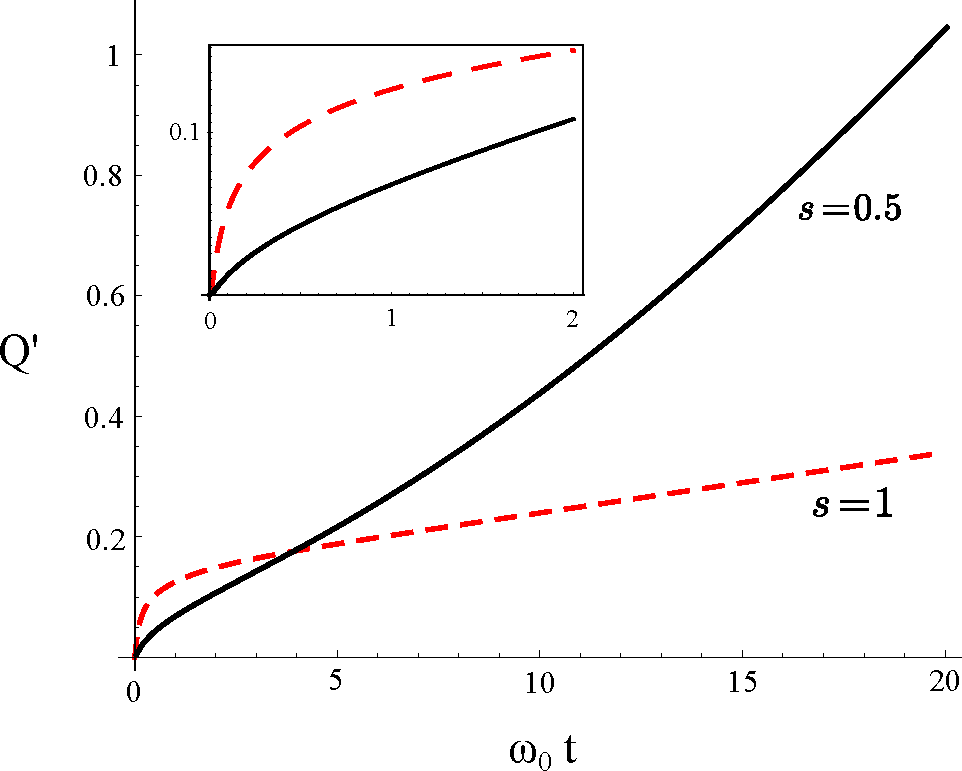
An effective microscopical description of the dissipation is given by the celebrated Caldeira-Leggett model [1], in which a quantum particle is subject to the linear interaction with a reservoir of N independent quantum harmonic oscillators. In the thermodynamical limit N → ∞ the reservoir is called a heat bath. The so-called spectral density function J(ω), describing the dependence of the coupling on the frequency, is assumed to be of the form J ∝ ω^se^−ω/ωc, where ω_c is a high-frequency cut-off. The special case s = 1 describes the so-called Ohmic dissipation. In most cases the Ohmic dissipation gives a good description of the effects exerted by the thermal bath, such as in Josephson flux qubits [2].

However, sub-Ohmic environments (s < 1) are of interest both from experimental and theoretical point of view. For example in single electron tunneling the electromagnetic environment constituted by an RC transmission line is sub-Ohmic with s = 0.5 [2]. A sub-Ohmic environment with s = 0.5 can be also realized by capacitively coupling an RLC transmission line to a mesoscopic metal ring [3]. Further examples of sub-Ohmic environments are found in nanomechanical devices [4]. The sub-Ohmic case, for an unbiased bistable system at T = 0, is characterized by a phase transition from the delocalized to localized phase [5,6]. This means that, in right/left well state representation (|Ri〉, |Li〉), one has 〈σ_z〉 ≠ 0 at t → ∞. The sub-Ohmic regime is interesting also because of the larger relative weight of the low frequency modes with respect to the Ohmic case. This feature reproduces the 1/f-noise in the s → 0 limit, which constitutes an important decoherence source in superconducting qubits, due to the presence of impurities [7].

A particle confined in a double well potential is a paradigmatic example of a bistable system, both in classical and in quantum physics. The confining potential is characterized by two minima separated by a barrier of height ΔU. The most important information of interest in such a system is the population distribution dynamics across the two minima. Classically, the only mechanism which allows for passage from one well to the other is the thermally activated jump over the barrier. On the other hand, the peculiar feature of the quantum regime is the tunneling, which allows probability amplitudes to diffuse across the barrier. Recently, the dynamics of quantum bistable systems has gained renewed interest [8–12].

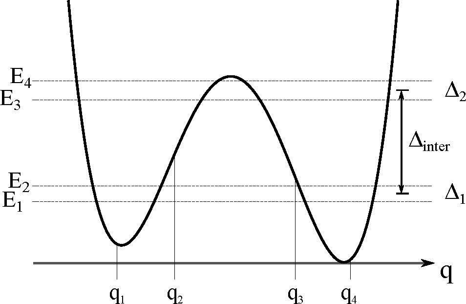
The strong nonlinearity of the potential causes the energy levels below the potential barrier to group into well-separated doublets. If the temperature is much smaller than the inter-doublet separation (Δ_inter, see Figure 1) between the first two doublets, then the system can be considered as an effective two-level system (TLS). The resulting dissipative TLS model is the so-called spin-boson (SB) model [13], as the excitations of the reservoir obey the Bose–Einstein statistics.

In the intermediate to high temperature regime, with respect to Δ_inter, and for initial preparations involving higher energies, the TLS approximation breaks down and the next-lying energy states are involved. Contrary to the SB model, which has been studied in every dissipation regime, both Ohmic and non-Ohmic [2,13–16], dissipative multi-state systems, beyond the weak coupling regime, have been less investigated, especially for non-Ohmic environments.

The reason is that the traditional Born-Markov master equation techniques, specifically the Bloch-Redfield master equation [17–19], which are perturbative in the system-bath coupling, describe well the weak coupling regime. However, whenever the coupling cannot be treated as a perturbation these techniques fail. The path integral approach, being non-perturbative in the coupling with the environment, is well suited in the intermediate to strong coupling regimes. An effective approach is based on numerical ab initio evaluations [20]. However, when the Hilbert space dimension of the system goes beyond two and the memory time of the reservoir becomes too large, this technique requires large computational resources. Indeed, the memory time of such non-markovian dynamics is typically very long for weak/intermediate coupling and low temperatures. Here we use an alternative path integral approach based on an integro-differential equation (see Ref. [2]) which is of the Nakajima-Zwanzig type [19] with approximate kernels.

In the TLS case the dicotomic nature of the paths in the left/right state representation makes the sum over paths possible for the free system and allows for approximate treatments of the environmental influences. On the other hand, in the general case of a M-state system, the variety of paths to be considered makes the evaluation of the kernel matrix a hard task independently of the dissipation regime considered. Therefore, further approximations on the contributing paths are needed.

Following Ref. [21] we consider a temperature/coupling regime where we can neglect a whole class of paths of the reduced density matrix (RDM), namely the paths with long off-diagonal excursions [22] (clusters), due to the cut-off operated by the thermal bath.

2. The Model

The system is a particle of mass M, coordinate $\widehat{q}$, and momentum $\widehat{p}$, subject to a double well potential V₀. The particle is linearly coupled to an environment of N independent quantum harmonic oscillators of frequencies ω_j, which, in the thermodynamical limit N → ∞, is the so-called bosonic heat bath.

The full Hamiltonian is the sum of a free system term, a free reservoir term and a system-reservoir interaction term

$$\widehat{H}=\frac{{\widehat{p}}^2}{2M}+V_0(\widehat{q})+{\displaystyle \sum _{j=1}^N\frac{1}{2}\left[\frac{{\widehat{p}}_j^2}{m_j}+m_j{\omega }_j^2{\left({\widehat{x}}_j-\frac{c_j}{m_j{\omega }_j^2}\widehat{q}\right)}^2\right]}.$$

(1)

The Hamiltonian has a renormalization term ∝${\widehat{q}}^2$ giving a spatially homogeneous dissipation, not depending on the particle’s coordinate $\widehat{q}$. The result is a so-called purely dissipative bath.

The interaction of the particle with the individual degrees of freedom of the reservoir is defined by the set of constants c_j and is proportional to the inverse of the reservoir’s volume [2]. Thus, for a macroscopic environment, the coupling with the individual oscillators is weak, which justifies the linear coupling assumption. Nevertheless, the overall influence exerted by the heat bath as a whole can be strong.

The bath spectral density function, which describes the frequency distribution of the reservoir’s oscillators and their coupling with the particle, is defined by

$$J(\omega )=\frac{\pi }{2}{\displaystyle \sum _{j=1}^N\frac{c_j^2}{m_j{\omega }_j}\delta (\omega -{\omega }_j)}$$

(2)

and has the dimension of mass times frequency squared.

In the general case of continuous bath the spectral density function is modeled as a power of ω, characterized by the exponent s, with an exponential cutoff at ω_c

$$J\left(\omega \right)=M\gamma {\omega }_{\mathrm{ph}}^{1-s}{\omega }^s{e}^{-\omega /{\omega }_c}.$$

(3)

The bath is said sub-Ohmic for 0 < s < 1, Ohmic for s = 1 and super-Ohmic for s > 1. The so-called damping constant γ is a measure, in the continuous limit, of the system-bath coupling.

The phonon frequency ω_ph is introduced in such a way that γ has the dimension of a frequency also in the non-Ohmic case (s ≠ 1). The exponential cut-off at high-frequency is introduced to avoid non-physical results as, for example, the divergence of the renormalization term in the Hamiltonian of Equation (1). The effect of the high frequency modes is taken into account by a redefinition of the particle’s bare mass, which is dressed by the high-frequency bath modes [2].

Within the Caldeira-Leggett model (see Equation (1)), the Heisenberg equation for the particle’s position operator results in the following generalized quantum Langevin equation [2,23]

$$M\ddot{\widehat{q}}(t)+M{\displaystyle {\int }_0^{t}d{t}^{\prime }\gamma (t-t^{\prime })\frac{d}{d{t}^{\prime }}\widehat{q}(t^{\prime })}+\frac{dV(\widehat{q}(t))}{d\widehat{q}(t)}=-M\gamma (t)\widehat{q}(0)+\widehat{\xi }(t),$$

(4)

where

$$\gamma (t)=\mathrm{\Theta }(t)\frac{1}{M}{\displaystyle \sum _{j=1}^N\frac{c_j^2}{m_j{\omega }_j^2}\cos ({\omega }_{j}t)}$$

(5)

$$\widehat{\xi }(t){\displaystyle \sum _{j=1}^N{c}_j}\left[{\widehat{x}}_j(0)\cos ({\omega }_{j}t)+\frac{{\widehat{p}}_j(0)}{m_j{\omega }_j}\sin ({\omega }_{j}t)\right]$$

(6)

are respectively the memory-friction kernel and the bath force operator. The expectation value of the bath force operator and the bath force autocorrelation, taken with respect to the environment in the canonical equilibrium state ${\rho }_{th}^R=Z^{-}{}^1\exp \left(-\beta {\widehat{H}}_R\right)$, are

$$\begin{array}{l}\begin{array}{cc}\langle \widehat{\xi }(t)\rangle R=T{r}_R\left[{\rho }_{th}^R\widehat{\xi }(t)\right]=0& \text{and}\end{array}\\ \langle \widehat{\xi }(t)\xi (\widehat{0})\rangle R=T{r}_R\left[{\rho }_{th}^R\widehat{\xi }(t)\widehat{\xi }(0)\right]=\frac{\hslash }{\pi }{\displaystyle {\int }_0^{\infty }d\omega }J(\omega )\left[\coth \left(\frac{\hslash \omega \beta }{2}\right)\cos (\omega t)-i\sin (\omega t)\right],\end{array}$$

(7)

respectively.

In the classical limit ( $\hslash \to 0$) the bath force correlation function is

$$\underset{\hslash \to \infty }{\lim }{\langle \widehat{\xi }(t)\xi (\widehat{0})\rangle }_R=\frac{1}{\beta }{\displaystyle \sum _{j=1}^N\frac{c_j^2}{m_j{\omega }_j^2}\cos ({\omega }_{j}t)}=M{k}_{B}T\gamma (t),$$

(8)

where we used coth(βħω_j/2) ∼ 2(βħω_j)⁻¹ for ħ → 0. Therefore the two relations in Equation (7), in the continuum limit (N → ∞), describe a stochastic force which in turn reproduce, in the classical limit, a classical colored noise source. In other words, non-Ohmic environments correspond to classical colored noise sources [24]. By comparing Equation (5) with Equation (2) and taking the continuous limit one finds that the Ohmic case gives, in the classical limit, a white noise source. Note that in the right hand side of the quantum Langevin equation (4) a term is dependent on the initial condition $\widehat{q}(0)$. This term is ascribable to the factorized initial condition with the reservoir in the canonical equilibrium and vanishes at long time due to the interference of the quasi-continuum of spectral components of γ(t).

3. Path Integral Representation of the Reduced Dynamics

We denote by $\mathcal{W}$ the full density matrix, characterized by the unitary evolution

$$\mathcal{W}\left(t\right)=U\left(t,t_0\right)\mathcal{W}\left(t_0\right)U^{†}\left(t,t_0\right),$$

where the time evolution operator is induced by the Hamiltonian (1).

The RDM, in the $\widehat{q}$ representation, reads

$${\rho }_{q{q}^{\prime }}\left(t\right)=\langle q|T{r}_B\mathcal{W}\left(t\right)|q^{\prime }\rangle .$$

We assume the following factorized initial condition

$$\mathcal{W}\left(t_0\right)=\rho \left(t_0\right)\otimes {\rho }_{th}^R.$$

(9)

With this initial condition, the dynamics of the RDM is given by the exact formal expression

$${\rho }_{q{q}^{\prime }}(t){\displaystyle \int d{q}_0}{\displaystyle \int d{q}_0^{\prime }G(q,q^{\prime }t;q_0,q_0^{\prime },t_0)}{\rho }_{q0q_0^{\prime }}(t_0),$$

(10)

where the propagator G is a double path integral in the left (right) coordinate q (q′)

$$G(q,q^{\prime }t;q_0,q_0^{\prime },t_0)={\displaystyle {\int }_{q(t_0)=q_0}^{q(t)=q}{\mathcal{D}}_q}{\displaystyle {\int }_{q^{\prime }(t_0)=q_0^{\prime }}^{q^{\prime }(t)=q^{\prime }}\mathcal{D}*q^{\prime }{e}^{\frac{i}{\hslash }(S[q]-S[q^{\prime }])}{F}_{FV}[q,q^{\prime }]}.$$

(11)

The transition amplitudes for paths with fixed extrema $\left(q_0,q_0^{\prime }\right)\to \left(q,q^{\prime }\right)$, in this sum-over-paths, are factorized as a bare system amplitude times the Feynman-Vernon influence functional F_FV. This functional accounts for the influence of the environment [25] and tends to 1 for vanishing γ.

3.1. Feynman-Vernon Influence Functional in the Discrete Variable Representaion

The exact path integral expression (11) for the propagator can be computed only in special cases, namely the free particle and the dissipative harmonic oscillator [26]. In the presence of nonlinear potentials, approximate treatments exist based on spatial discretization, attained by restricting the Hilbert space of the open system [27]. Specifically, based on the assumption that, given the initial condition and the damping/temperature regime, the system is not likely to visit high-energy states during its time evolution, the Hilbert space of the system is restricted to that spanned by the first M energy eigenstates. Thus the problem reduces to that of a dissipative M-state system. In the present work we consider the so called double-doublet system, in which the first M = 4 levels of the quartic potential [22]

$$V_0(\widehat{q})=\frac{M^2{\omega }_0^4}{64\mathrm{\Delta }U}{\widehat{q}}^4-\frac{M{\omega }_0^2}{4}{\widehat{q}}^2-ϵ\widehat{q}$$

(12)

are considered.

The discrete variable representation (DVR) is then obtained by diagonalizing the position operator in this restricted Hilbert space. The continuum of position states turns into a discrete set of states localized around a grid of 4 position eigenvalues q₁,…, q₄, where

$$\widehat{q}|q_j\rangle =q_j|q_j\rangle .$$

(13)

In this picture, the paths of the coordinates q and q′ are represented by a sequence of transitions among the positions q_j. In Figure 1 the potential considered in this work, the first four energy levels, and the position eigenvalues are shown.

From now on we consider the time evolution of the populations ρ_ii = 〈q_i|ρ|q_i〉, i.e., the diagonal elements of the RDM in the DVR. Taking the influence functional as ${\mathrm{F}}_{FV}=\exp \left(-{\mathrm{\Phi }}_{FV}\right)$, the influence phase in the DVR for a path with N transitions at times t₁, …, t_N has the following form

$${\mathrm{\Phi }}_{FV}\left[\xi ,\chi \right]=-{\displaystyle \sum _{i=1}^N{\displaystyle \sum _{j=0}^{i-1}\left[{\xi }_i{Q}^{\prime }(t_i-t_j){\xi }_j+i{\xi }_i{Q}^{″}(t_i-t_j){\chi }_j\right]}},$$

(14)

where the stepwise functions of time ξ_i and χ_i are the so called charges

$$\begin{array}{l}{\xi }_j=\left(q_j-q_{j-}{}_1\right)-\left(q_j^{\prime }-q_{j-1}^{\prime }\right)\\ {\chi }_j=\left(q_j-q_{j-}{}_1\right)+\left(q_j^{\prime }-q_{j-1}^{\prime }\right)\end{array}$$

(15)

and the indexes refer to the transition times.

The time-integrated bath correlation function Q(t) = Q′(t) + iQ″(t), also called pair interaction because it couples the charges at different times, is related to the bath autocorrelation function by $\ddot{Q}(t)={\langle \widehat{\xi }(t)\xi (\widehat{0})\rangle }_R/{\hslash }^2$. Its general expression is

$$\begin{array}{c}Q(t)=\frac{M{\gamma }_s}{\pi \hslash }{\left(\frac{{\omega }_c}{{\omega }_{\mathrm{ph}}}\right)}^{s-1}\Gamma \left(s-1\right)\{1-{(1+i{\omega }_{c}t)}^{1-s}+2{(\hslash \beta {\omega }_c)}^{1-s}\zeta (s-1,1+\kappa )\\ -{(\hslash \beta {\omega }_c)}^{1-s}[\zeta (s-1,1+\kappa +i\kappa {\omega }_{c}t)+\zeta (s-1,1+\kappa -i\kappa {\omega }_{c}t)]\},\end{array}$$

(16)

where the dimensionless quantity κ is defined by κ = (ħβω_c)⁻¹. The function Γ(z) is the Euler gamma function and ζ(z, q) is the Hurwitz zeta function $\zeta \left(z,q\right)={\displaystyle {\sum }_{n=0}^{\infty }1/{\left(q+n\right)}^z}$, related to the Riemann zeta function ζ(z) by ζ(z) ≡ ζ(z, 1).

3.2. Generalized Non-interacting Blip Approximation

According to the path integral jargon, a blip is an off-diagonal configuration of an RDM path for two-level systems, while, for M-state systems an off-diagonal excursion of an RDM path is called cluster. From the expression for the phase Φ_FV (Equation (14)) the influence functional ${\mathrm{F}}_{FV}=\exp \left(-{\mathrm{\Phi }}_{FV}\right)$ is time non-local as it couples the ξ- and χ-charges at every transition time. This feature prevents an exact evaluation of the path integral expression for the populations. Nevertheless a multi-state generalization of the non-interacting blip approximation (NIBA) exists, known as generalized non-interacting cluster approximation (gNICA) [21]. For Ohmic friction, in the high temperature limit, the function Q(t) assumes a linearized form at short times. This implies an almost exact decoupling of the clusters. Moreover if the damping γ is sufficiently strong one can retain, in the sum over paths, the leading contributions given by RDM paths with clusters consisting of single off-diagonal transitions or blips. The gNICA scheme to the leading order can thus be called gNIBA (generalized NIBA).

In the sub-Ohmic case the decoupling of the blips is attained at shorter times, and long clusters are suppressed more effectively with respect to the Ohmic case, due to stronger cut-off operated by Q′ in the real part of Φ_FV. These two features make the gNIBA more accurate in the sub-Ohmic than in the Ohmic regime. This can be seen from Figure 2, where the real part of Q is shown as a function of time for s = 1 and 0.5, i.e., in the Ohmic and sub-Ohmic regimes, respectively.

The cut-off localizes in time the influence of the environment, which results in the factorization of the path integral expression for the propagator in Laplace space. This allows to obtain a generalized master equation for the populations in the DVR [28] which, for the double-doublet system (M = 4), reads

$${\dot{\rho }}_{ii}(t)={\displaystyle \sum _{j=1}^4{\displaystyle {\int }_{t_0}^{t}d{t}^{\prime }{K}_{ij}(t-t^{\prime })}}{\rho }_{jj}(t^{\prime }).$$

(17)

The non-diagonal elements of the gNIBA approximated kernel matrix K are

$$K_{ij}(t)=2{\mathrm{\Delta }}_{ij}^2{e}^{-q_{ij}^2{Q}^{\prime }(t)}\cos \left({ϵ}_{ij}t+q_{ij}^2{Q}^{″}(t)\right),$$

(18)

where

$$\begin{array}{l}{\mathrm{\Delta }}_{ij}=\frac{1}{\hslash }\langle q_i|{\widehat{H}}_S|q_j\rangle ,\\ {ϵ}_{ij}=\frac{1}{\hslash }\left(\langle q_i|{\widehat{H}}_S|q_i\rangle -\langle q_j|{\widehat{H}}_S|q_j\rangle \right),\\ q_{ij}^2={\left(q_i-q_j\right)}^2,\end{array}$$

with Ĥ_S the bare system Hamiltonian.

The diagonal elements of K are given by the probability conservation

$$K_{ii}(t)=-{\displaystyle \sum _{\begin{array}{c}j=1\\ j\ne i\end{array}}^4{K}_{ji}(t)}.$$

(19)

4. Results

In this section, we show the dynamics of the populations in the DVR, the spatially localized representation introduced in Section 3.1. The results are obtained by numerically integrating the generalized master equation given in Equation (17).

The quantum particle is subject to the biased bistable potential in Figure 1. The barrier height (at zero bias) and the bias are ΔU = 1.4 ħω₀ and $ϵ=0.02\sqrt{M\hslash {\omega }_0^3}$, respectively. The frequency ω₀ ∼ Δ_inter/ħ is the natural oscillation frequency around the potential minima (see Equation (12) and Figure 1).

Due to the asymmetry of the potential, at equilibrium we expect that P ≡ P_R − P_L > 0, where the left and right well population are defined by P_L = ρ₁₁ + ρ₂₂ and P_R = ρ₃₃ + ρ₄₄. The value of the population difference P depends on the temperature and damping strength γ.

We consider the sub-Ohmic regime with s = 0.5. The cut-off frequency is set at ω_c = 50 ω₀ and the phonon frequency at ω_ph = ω₀ (see Equation (3)). The generalized master equation given in Equation (17) is numerically solved for two temperatures, namely T = 0.2, 0.3 ħω/k_B. In all graphs shown in this section the system is initially in the out-of-equilibrium state ρ(0) = |q₁〉〈q₁|, that is the particle is initially prepared as a wave packet centered at the position q₁ (see Figure 1). This initial condition involves the states belonging to the higher energy doublet, implying that the TLS approximation is not valid whatever the temperature regime is.

The energy levels structure, shown in Figure 1, implies that the bare system has multiple time scales: a fast one, of the order of the inverse of the inter-doublet separation ħ/Δ_inter, and a slower one, of the order of the intra-doublet separation ħ/Δ₁ ∼ ħ/Δ₂. Notice that, due to the bias, the intra-doublet separation are of the same order, while in the unbiased (symmetric potential) case we have Δ₁ << Δ₂ [29].

In this section, both in the text and figure, temperatures and damping strengths are expressed in units of ħω₀/k_B and ω₀, respectively.

4.1. Dynamics of the Populations

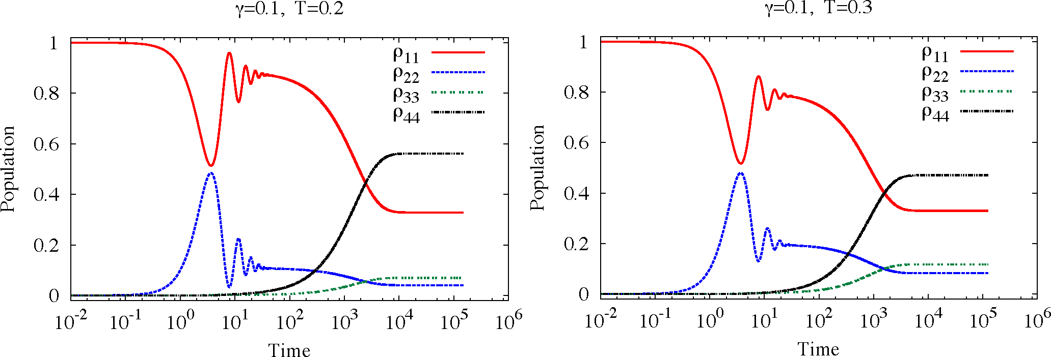
Because the coupling with the environment is in the intermediate to strong regime, the slow tunneling dynamics is incoherent. This means that the oscillations between the two wells, predicted for the free system, are completely damped out. The reason is twofold: (i) transitions among populations of distant DVR states |q_i〉 and |q_j〉 are suppressed more effectively, due to the prefactor $q_{ij}^2$ in the exponential cutoff of the gNIBA kernels (Equation (18)); (ii) the energy scale Δ₁ ∼ Δ₂ of the tunneling dynamics is smaller than that of the intra-well dynamics (given by the inter-doublet separation Δ_inter). The effective damping is therefore strong on the scale of tunneling separation and intermediate on the scale of the inter-doublet separation. As a consequence, while the intra-well dynamics displays a damped oscillatory behavior, the tunneling dynamics is overdamped. This crossover dynamical regime, found also for Ohmic damping in Ref. [29], is shown in Figure 3 where two values of the temperature, T = 0.2 and 0.3, are considered with γ fixed to the value 0.1.

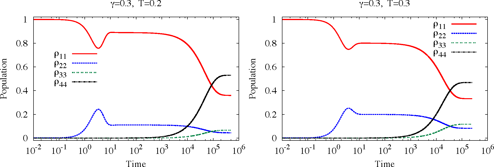
Figure 4 shows the time evolution of the populations at the stronger damping γ = 0.3. The dynamics occurs at the transition between the crossover and the completely incoherent regimes. This transition from coherent to incoherent dynamics has been investigated for the sub-Ohmic spin-boson in Ref. [30]. At both temperatures investigated, the prediction is that no full intra-well oscillation in the transient takes place. Moreover the relaxation times, at both temperatures, are larger for this value of γ with respect to that considered in Figure 3.

Note that, due to the difference in time scales between the intra- and inter-well dynamics, the intra-well relaxation of the left well populations occurs before the tunneling takes place and a sort of metastability appears during the transient before the relaxation to the equilibrium takes place. A similar behavior, but of different nature, has been found in Ref. [31]. There, for a symmetric two-level system in the sub-Ohmic regime, a slowly decaying quasiequilibrium state is present during the transient, due to a shifted initial preparation. This kind of shifted equilibrium initial condition is of experimental interest and is worth investigating for multi-state systems in sub-Ohmic baths in future developments.

Finally, both in Figures 3 and 4, the internal states |q₂i〉 and |q₃〉, with wave packets centered away from the potential minima (see Figure 1), are more populated at the higher temperature. This effect is evident at the lower value of damping (Figure 3). The reason is that: (i) at equilibrium, the higher doublet of energy states is relatively more populated at T = 0.3 than at T = 0.2; (ii) the energy states of the higher doublet contribute more to the internal DVR states than to the external ones (|q₁〉 and |q₄〉, centered near the minima). As a consequence. ${\rho }_{22/33}^{\mathrm{eq}}\left(T=0.3\right)>{\rho }_{22/33}^{\mathrm{eq}}\left(T=0.2\right)$.

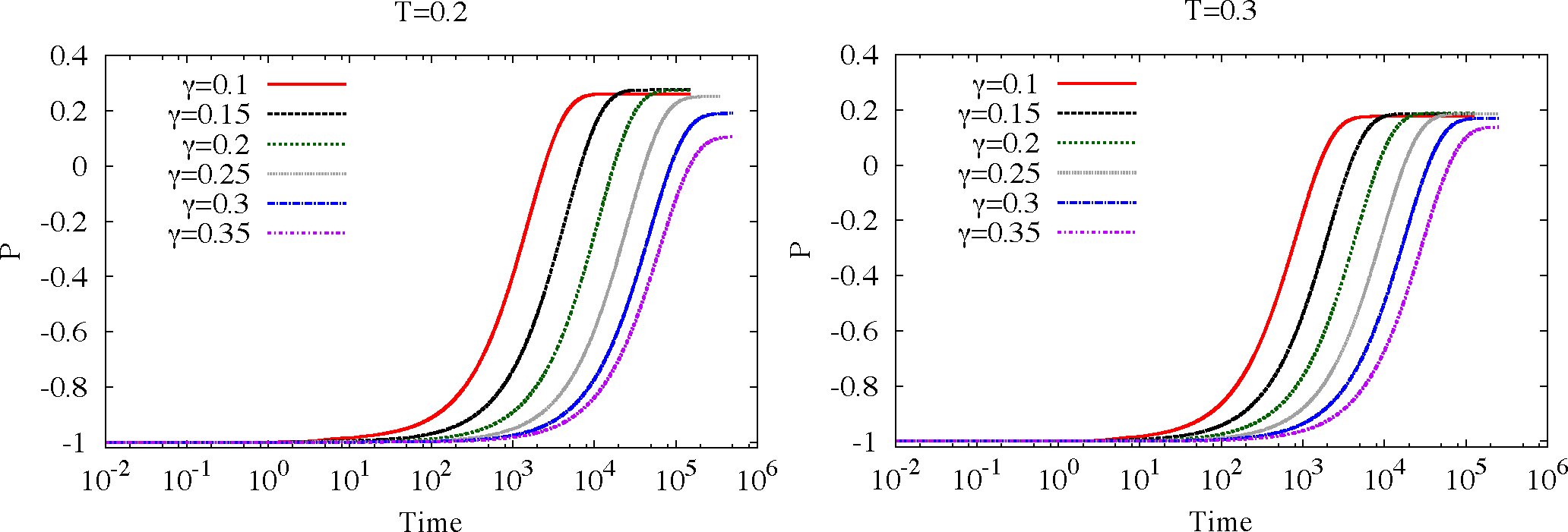
4.2. Population Difference—Time Evolution and Equilibrium Configuration

In this section, we study the time evolution and stationary configuration of the population difference P = P_R − P_L. In Figure 5 we plot P as a function of time, for the two temperatures T = 0.2, 0.3 and different values of γ.

The intra-well oscillations of ρ₁₁ and ρ₂₂, shown in Figures 3 and 4, are not visible in Figure 5. This is because we consider the overall left/right well populations. The time evolution of P is a monotonic relaxation towards an equilibrium configuration which depends on the temperature and damping strength.

All plots have qualitatively the same features but are shown to highlight how the relaxation time and the equilibrium value of P behave, at the considered temperatures, with respect to an increase of the coupling with the environment, which is quantified by γ.

Specifically, at T = 0.2, 0.3, the relaxation time grows exponentially with γ, at least around γ = 0.1 (notice that the plot is in log-scale). This behavior is similar to that predicted for Ohmic damping [21,32].

As expected, for fixed γ, P (t → ∞) is higher at the lower temperature T = 0.2, which indicates that the probability to find the particle in the left well at equilibrium is lower at this value of temperature with respect to the higher value T = 0.3.

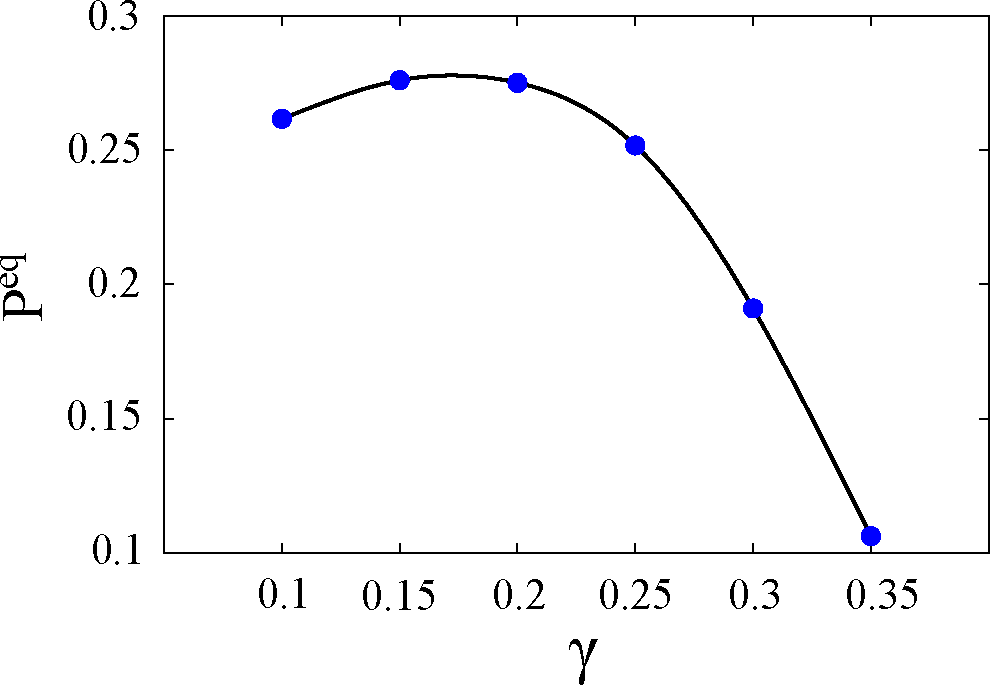
Moreover, P ^eq ≡ P (t → ∞) behaves nontrivially with respect to the coupling, especially at T = 0.2 (Figure 5, left panel), as shown in Figure 6 where P ^eq is plotted as a function of γ. The curve displays a maximum around γ = 0.15. This prediction may be ascribed to the multi-level nature of the system studied. Specifically, two competing effects are present. On the one hand, an increase of the coupling forces the relaxation towards the lower well, producing an increase of P ^eq. On the other hand, the higher energy doublet gets more populated and the effective damping is reduced, with a corresponding decrease of P ^eq. The combined effect of these two mechanisms is a possible explanation of the nonmonotonicity found. This result, together with the multiple dynamical time scales and the appearance of the so-called vibrational relaxation (intra-well motion), is another peculiar feature of the picture arising from treating the system beyond the TLS approximation.

5. Conclusions

In this work, we investigate the relaxation dynamics and the equilibrium configuration of a biased bistable system in a strongly dissipative sub-Ohmic environment. We consider an out of equilibrium initial condition, with the particle localized in the higher well of the bistable potential. The time evolution of the populations in a space localized representation is calculated by using a real-time path integral approach. A NIBA-like approximation scheme has been used which is suitable for the dissipation regimes considered, especially for a sub-Ohmic spectral density.

The system is studied beyond the two-level system approximation. Specifically the Hilbert space is restricted to that spanned by the states belonging to the first two energy doublets. This feature, along with the specific initial condition chosen, results in the presence of multiple time scales in the relaxation dynamics. We observe a crossover dynamical regime, characterized by damped intra-well oscillations and incoherent tunneling, at intermediate damping. At strong damping the dynamics makes a transition to the completely incoherent relaxation.

The study, performed for two different values of temperature, shows a dependence of the stationary configuration on the temperature and on the damping strength. Specifically, at fixed damping, the higher well is more populated at the higher temperature while, at fixed temperature, the left well has a minimum of the population when the damping value roughly coincides with the higher intra-doublet frequency spacing. This result, along with the observation of intra- and inter-well dynamics, is a peculiar feature of treating the system beyond the two-level system approximation.

References

1. Caldeira, A.O.; Leggett, A.J. Influence of Dissipation on Quantum Tunneling in Macroscopic Systems. Phys. Rev. Lett. 1981, 46, 211–214. [Google Scholar]
2. Weiss, U. Quantum Dissipative Systems, 4th ed.; World Scientific: Singapore, Singapore, 2012. [Google Scholar]
3. Tong, N.H.; Vojta, M. Signatures of a Noise-Induced Quantum Phase Transition in a Mesoscopic Metal Ring. Phys. Rev. Lett. 2006, 97, 016802. [Google Scholar]
4. Seoanez, C.; Guinea, F.; Neto, A.H.C. Dissipation due to two-level systems in nano-mechanical devices. Europhys. Lett. 2007, 78, 60002. [Google Scholar]
5. Le Hur, K.; Doucet-Beaupré, P.; Hofstetter, W. Entanglement and Criticality in Quantum Impurity Systems. Phys. Rev. Lett. 2007, 99, 126801. [Google Scholar]
6. Wang, H.; Thoss, M. From coherent motion to localization: II. Dynamics of the spin-boson model with sub-Ohmic spectral density at zero temperature. Chem. Phys. 2010, 370, 78–86. [Google Scholar]
7. Paladino, E.; Galperin, Y.M.; Falci, G.; Altshuler, B.L. 1/f noise: Implications for solid-state quantum information. Rev. Mod. Phys. 2014, 86, 361–418. [Google Scholar]
8. Bera, S.; Florens, S.; Baranger, H.U.; Roch, N.; Nazir, A.; Chin, A.W. Stabilizing spin coherence through environmental entanglement in strongly dissipative quantum systems. Phys. Rev. B 2014, 89, 121108. [Google Scholar]
9. Kast, D.; Ankerhold, J. Persistence of Coherent Quantum Dynamics at Strong Dissipation. Phys. Rev. Lett. 2013, 110, 010402. [Google Scholar]
10. Chin, A.W.; Prior, J.; Huelga, S.F.; Plenio, M.B. Generalized Polaron Ansatz for the Ground State of the Sub-Ohmic Spin-Boson Model: An Analytic Theory of the Localization Transition. Phys. Rev. Lett. 2011, 107, 160601. [Google Scholar]
11. Magazzù, L.; Valenti, D.; Caldara, P.; La Cognata, A.; Spagnolo, B.; Falci, G. Transient Dynamics and Asymptotic Populations in a Driven Metastable Quantum System. Acta Phys. Pol. B 2013, 44, 1185. [Google Scholar] [Green Version]
12. Spagnolo, B.; Caldara, P.; La Cognata, A.; Valenti, D.; Fiasconaro, A.; Dubkov, A.A.; Falci, G. The bistable potential: an archetype for classical and quantum systems. Int. J. Mod. Phys. B 2012, 26, 1241006. [Google Scholar]
13. Leggett, A.J.; Chakravarty, S.; Dorsey, A.T.; Fisher, M.P.A.; Garg, A.; Zwerger, W. Dynamics of the dissipative two-state system. Rev. Mod. Phys. 1987, 59, 1–85. [Google Scholar]
14. Bulla, R.; Costi, T.; Pruschke, T. Numerical renormalization group method for quantum impurity systems. Rev. Mod. Phys. 2008, 80, 395–450. [Google Scholar]
15. Alvermann, A.; Fehske, H. Sparse Polynomial Space Approach to Dissipative Quantum Systems: Application to the Sub-Ohmic Spin-Boson Model. Phys. Rev. Lett. 2009, 102, 150601. [Google Scholar]
16. Nesi, F.; Paladino, E.; Thorwart, M.; Grifoni, M. Spin-boson dynamics beyond conventional perturbation theories. Phys. Rev. B 2007, 76, 155323. [Google Scholar]
17. Morillo, M.; Denk, C.; Cukier, R. Control of tunneling reactions with an external field in a four-level system: A general Redfield approach. Chem. Phys. 1996, 212, 157–175. [Google Scholar]
18. Cukier, R.; Denk, C.; Morillo, M. Control of tunneling processes with an external field in a four-level system: an analytic approach. Chem. Phys. 1997, 217, 179–199. [Google Scholar]
19. Breuer, H.P.; Petruccione, F. The Theory of Open Quantum Systems; Oxford University Press: Oxford, UK, 2002. [Google Scholar]
20. Makri, N.; Makarov, D. Tensor propagator for iterative quantum time evolution of reduced density matrices. I. Theory. J. Chem. Phys. 1995, 102, 4600–4610. [Google Scholar]
21. Thorwart, M.; Grifoni, M.; Hänggi, P. Strong Coupling Theory for Tunneling and Vibrational Relaxation in Driven Bistable Systems. Ann. Phys. 2001, 293, 15–66. [Google Scholar]
22. Thorwart, M.; Grifoni, M.; Hänggi, P. Strong Coupling Theory for Driven Tunneling and Vibrational Relaxation. Phys. Rev. Lett. 2000, 85, 860–863. [Google Scholar]
23. Hänggi, P.; Ingold, G.L. Fundamental aspects of quantum Brownian motion. Chaos 2005, 15, 026105. [Google Scholar]
24. Hausinger, J. Dissipative dynamics of a qubit-oscillator system in the ultrastrong coupling and driving regime. Ph.D. Thesis, Universität Regensburg, Regensburg, Germany, 2010. [Google Scholar]
25. Feynman, R.P.; Vernon, F., Jr. The theory of a general quantum system interacting with a linear dissipative system. Ann. Phys. 1963, 24, 118–173. [Google Scholar]
26. Grabert, H.; Schramm, P.; Ingold, G.L. Quantum Brownian motion: the functional integral approach. Phys. Rep. 1988, 168, 115–207. [Google Scholar]
27. Harris, D.O.; Engerholm, G.G.; Gwinn, W.D. Calculation of Matrix Elements for One-Dimensional Quantum-Mechanical Problems and the Application to Anharmonic Oscillators. J. Chem. Phys. 1965, 43, 1515–1517. [Google Scholar]
28. Grifoni, M.; Sassetti, M.; Weiss, U. Exact master University for driven dissipative tight-binding models. Phys. Rev. E 1996, 53, R2033–R2036. [Google Scholar]
29. Magazzù, L.; Valenti, D.; Spagnolo, B.; Grifoni, M. Dissipative dynamics in a quantum bistable system: crossover from weak to strong damping 2014, arXiv, 1412.7467v1.
30. Nalbach, P.; Thorwart, M. Crossover from coherent to incoherent quantum dynamics due to sub-Ohmic dephasing. Phys. Rev. B 2013, 87, 014116. [Google Scholar]
31. Nalbach, P.; Thorwart, M. Ultraslow quantum dynamics in a sub-Ohmic heat bath. Phys. Rev. B 2010, 81, 054308. [Google Scholar]
32. Caldara, P.; La Cognata, A.; Valenti, D.; Spagnolo, B.; Berritta, M.; Paladino, E.; Falci, G. Dynamics of a quantum particle in asymmetric bistable potential with environmental noise. Int. J. Quantum Inf. 2011, 9, 119–127. [Google Scholar]
Figure 1. Potential V0 (see Equation (12)) with ΔU = 1.4 ħω0 and ϵ = 0.02 M ħ ω 0 3. The intra-doublet separations are Δ1 ≃ 0.12 ħω0 and Δ2 ≃ 0.15 ħω0, while the inter-doublet spacing is Δinter = (E4 + E3E2E1)/2 ≃ 0.814 ħω0.
Entropy 17 02341f1
Figure 2. (Color online) Real part of the function Q (Equation (16)) vs time for s = 0.5 (sub-Ohmic) and s = 1 (Ohmic). The damping strength is γ = 0.1 ω0 and the temperature T = 0.1 ħω0/kB. The inset shows the behavior of Q′ at short times.
Entropy 17 02341f2
Figure 3. Time evolution of the four populations ρii in the intermediate damping regime γ = 0.1 ω0 for sub-Ohmic damping (s = 0.5). Left panelT = 0.2. Right panelT = 0.3. Both the evolutions display a transient with coherent intra-well oscillations and an incoherent inter-well (tunneling) dynamics. At higher temperature (right panel) the left well population (ρ11 + ρ22) is larger than that at the lower temperature (left panel). Temperatures and γ are given in units of ħω0/kB and ω0, respectively. Time is in units of ω 0 1.
Entropy 17 02341f3
Figure 4. Time evolution of the four populations ρii in the strong damping regime γ = 0.3 for sub-Ohmic damping (s = 0.5). Left panelT = 0.2. Right panelT = 0.3. The coherent intra-well oscillations are damped and the relaxation dynamics is in the transition from the crossover to the completely incoherent relaxation regime. As well as for γ = 0.1 (Figure 3), at higher temperature (right panel) the left well population (ρ11 + ρ22) is larger than that at the lower temperature (left panel). Temperatures and γ are given in units of ħω0/kB and ω0, respectively. Time is in units of ω 0 1.
Entropy 17 02341f4
Figure 5. Time evolution of the population difference P = PR − PL in the sub-Ohmic dissipation regime (s = 0.5), for different values of γ, at T = 0.2 (left panel) and T = 0.3 (right panel). Temperatures and γ are given in units of ħω0/kB and ω0, respectively. Time is in units of ω 0 1.
Entropy 17 02341f5
Figure 6. Population difference at equilibrium Peq = P (t → ∞) as a function of γ (in units of ω0) at temperature T = 0.2 ħω0/kB (see left panel of Figure 5). 5. Conclusions
Entropy 17 02341f6