On Nonlinear Complexity and Shannon’s Entropy of Finite Length Random Sequences

Abstract

Pseudorandom binary sequences have important uses in many fields, such as spread spectrum communications, statistical sampling and cryptography. There are two kinds of method in evaluating the properties of sequences, one is based on the probability measure, and the other is based on the deterministic complexity measures. However, the relationship between these two methods still remains an interesting open problem. In this paper, we mainly focus on the widely used nonlinear complexity of random sequences, study on its distribution, expectation and variance of memoryless sources. Furthermore, the relationship between nonlinear complexity and Shannon’s entropy is also established here. The results show that the Shannon’s entropy is strictly monotonically decreased with nonlinear complexity.

1. Introduction

Pseudorandom binary sequences have important uses in many fields, such as error control coding, spread spectrum communications, statistical sampling and cryptography [1–3]. A good random number generation will help to improve the results in these applications. At the beginning, most existing methods for generating pseudorandom bit sequences are based on the mid-square method, the linear congruential method, linear and nonlinear feedback shift registers, etc. These kinds of pseudorandom bit generators (PRBGs) are not secure enough for their inner fixed linear structure. The chaotic system is highly sensitive to its initial condition and parameters, together with its random-like and unpredictability, et al., is very useful in improving its security, and is better than the Linear Feedback Shift Register in the cryptographic properties. Therefore, in recent years, chaotic system is regarded as an important pseudorandom source in the design of random bit generators [4–9].

There are two kinds of method in evaluating the properties of sequences, one is based on the probability measure. Till now, many information-theoretic studies of pseudorandom sequences have been provided. In 1949, Shannon first introduced the concept of “entropy” from thermodynamics into information science, and proposed it as an uncertainty measure of random variables [10]. Kohda et al. [11] studied the statistical properties of binary sequences generated by a class of ergodic maps with some symmetric properties, and a simple sufficient condition for these maps to produce a sequence of independent and identically distributed binary random variables. They also evaluated the dependence of a chaotic real-valued trajectory generated by the Chebyshev map of degree k by using the N-th-order dependency moments, and find that the real-valued trajectory generated by the Chebyshev map of degree k has the k-th-order correlated property [12]. Visweswariah et al. [13] showed that under general conditions, the optimal variable-length source codes asymptotically achieve optimal variable-length random bit generation in a rather strong sense. Beirami et al. indicated that the entropy rate plays a key role in the performance and robustness of chaotic map truly random number generators [14], and provided converse and achievable bounds on the binary metric entropy [15], which is the highest rate at which information can be extracted from any given map using the optimal bit-generation function, and et al.

Besides using the probability measure to evaluate a random sequence, many researchers provided the so-called deterministic complexity measures. Among all these complexity measures, the following four measures may be the most important ones. They are linear complexity, Lempel-Ziv complexity, eigenvalues and nonlinear complexity, respectively [16–26]. Among these four measures, linear complexity and Lempel-Ziv complexity have achieved widely studied. However, the nonlinear complexity has not been studied to the same extents.

Both these two kinds of measure are used to measure the properties of random sequences. However, the relationship between them is still lack of studies [20,27,28]. Lempel et al. [20] established the relation between Lempel-Ziv complexity and normalized entropy of random binary sequence. The relationship between T-complexity and KS entropy for one-dimensional Logistic map is shown in [27]. Reference [28] shows the relationship between eigenvalue and Shannon’s entropy of random sequences. In this paper, we will study on the nonlinear complexity of random sequences generated by the memoryless sources. Furthermore, we will also provide that the nonlinear complexity is inverse correlated with Shannon’s entropy.

The rest of our paper is organized as follows. The expectation and variance of nonlinear complexity of random sequences are discussed in Section 2. In Section 3, we will establish the relationship between nonlinear complexity and Shannon’s entropy. Section 4 concludes the whole paper.

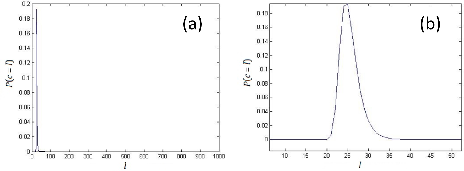
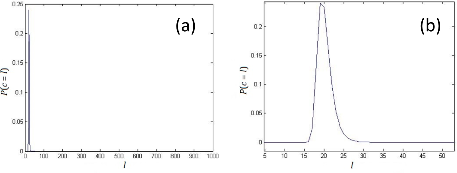
2. Nonlinear Complexity of Random Binary Sequences

First, we give some basic definitions. Let s = s₀, s₁, s₂, … be a sequence and s_i^j = s_i, …s_j, with i ≤ j, be its tuple. If s has finite length N, then s^N: = s₀^N−1 denotes the whole sequence. Any ultimately periodic sequence can be generated by a feedback shift register, satisfying a recurring relation

$$s_{i+n}=h(s_{i+n-1},s_{i+n-2},\dots ,s_i),i\ge 0$$

where n > 0 equals the length of the FSR. The function h is called the nonlinear feedback function. Nonlinear complexity, is defined as the minimum order of the FSR which can generate s^N, denoted as c(s^N). The sequence c(s¹), …, c(s^N) is called nonlinear complexity profile.

The minimal FSR of a sequence is not unique [26]. Therefore, it is not convenience to calculate the nonlinear complexity by using its definition. Usually, we use the following proposition to determine the nonlinear complexity of a given sequence. This proposition is taken from [25,26].

Proposition 1 ([25,26]): Let l be the length of the longest tuple in a sequence s^N that occurs at least twice with different successors. Then c(s^N) = l + 1.

This Proposition is valid if the constant term of the feedback function of the FSR is allowed to be nonzero. If we are confined to zero constant terms, then we have that c(s^N) = max{l + 1, m + 1}, where m is the length of the longest nonending run of zeros in s^N. Clearly m ≤ l + 1, since the existence of a run of m zeros followed by any nonzero element directly implies that l ≥ m − 1.

Proposition 1 shows that, if the nonlinear complexity of a sequence equals to l, then the following two conditions must hold, and vice versa.

• There exist a tuple with length l − 1, which occurs at least twice.
• All the tuples with length l do not occur more than once.

Consider a random binary sequence s^N = s₀, s₁, …, s_N−1 with its nonlinear complexity c(s^N) = l. Let the probability of symbol “0” occurs be Pr(0) = p. Then the probability of all the tuples with length l do not occur more than once can be written as

$$p(l)={(1-{(2p^2-2p+1)}^l)}^{C_{N-l+1}^2}$$

here, $C_{N-l+1}^2$ is the number of all possible two positions, where tuple of length l may occur simultaneously, 2p² − 2p + 1 is the probability which two arbitrary tuples of length 1 are the same. Therefore, according to conditions (1) and (2), the probability of c(s^N) = l can be calculated as

$$P(c(s^N)=l)={(1-{(2p^2-2p+1)}^l)}^{C_{N-l+1}^2}-{(1-{(2p^2-2p+1)}^{l-1})}^{C_{N-l+2}^2}$$

(1)

When p = 0.5, the sequence comes to be uniform, and the probability of c(s^N) = l can be simplified written as

$$P(c(s^N)=l)={(1-\frac{1}{2^l})}^{C_{N-l+1}^2}-{(1-\frac{1}{2^{l-1}})}^{C_{N-l+2}^2}$$

(2)

Let p = 0.3 and 0.5, respectively, and the length N = 1000, the probability distribution of nonlinear complexity of random binary sequences are shown in Figures 1 and 2. From these two figures we can see that, theoretically, the nonlinear complexity of a random binary sequence may be any integer which is smaller than the sequence’s length. However, the probability almost equals to zero except for a relatively narrow interval.

According to the probability distribution (1), the expectation of nonlinear complexity can be written as

$$E(c(s,p))={\displaystyle \sum _{l=1}^{N}l\cdot ({(1-{(2p^2-2p+1)}^l)}^{C_{N-l+1}^2}-{(1-{(2p^2-2p+1)}^{l-1})}^{C_{N-l+2}^2})}$$

(3)

If the sequence is uniformly distributed, with p = 0.5, then the expectation can be simplified written as

$$E(c(s^N))={\displaystyle \sum _{l=1}^{N}l}\cdot P(c(s^N)=l)={\displaystyle \sum _{l=1}^{N}l}\cdot ({(1-\frac{1}{2^l})}^{C_{N-l+1}^2}-{(1-\frac{1}{2^{l-1}})}^{C_{N-l+2}^2})$$

(4)

Jansen et al. [26] derived the expectation of nonlinear complexity for the sequences with alphabet of any cardinality. For binary sequences, the expectation approximately equals to 2log₂N. Figure 3 compares our result with the 2log₂N line, which shows that they are approximately the same for large N.

By calculating the value of E(c(s^N)) in Equation (4) and 2log₂N with different length N, we can get the following error e

$$e=E(c(s^N))-2{\log }_{2}N$$

The value of e with different length N is shown in Figure 4. From Figure 4 we have that, for moderate large N, the error will almost remain the same, which is about 0.3019. As we know, if the length N be a quite large number, then the value 0.3019 is rather small which can be ignored. Therefore, for moderate large N, the expectation of nonlinear complexity can be approximately written as

$$E(c(s^N))=2{\log }_{2}N+0.3019\approx 2{\log }_{2}N$$

(5)

Correspondingly, for a general random sequence with p ≠ 0.5, the expectation can be approximately written as

$$E(c(s,p))\approx 2{\log }_{1/(2p^2-2p+1)}N$$

(6)

for moderate large N.

Let p = 0.1, 0.2, 0.3, 0.4 and 0.5, respectively, we can compare the value of the expectation of nonlinear complexity of random sequences, as show in Figure 5. From Figure 5 we can find that, the expectations of nonlinear complexity profile have a clear hierarchy. The more uniform the sequence is, the smaller the expectation of nonlinear complexity is.

Next, we can derive the variance of nonlinear complexity of random sequences for moderate large N as

$$\mathrm{Var}(c(s,p))={\displaystyle \sum _{l=1}^N{(l-2{\log }_{1/(2p^2-2p+1)}N)}^2\cdot P(c(s^N)=l)}$$

(7)

where $P(c(s^N)=l)$ is given by (1).

If the sequence is uniformly distributed, with p = 0.5, then the variance can be simplified written as

$$\mathrm{Var}(c(s^N))={\displaystyle \sum _{l=1}^N{(l-2{\log }_{2}N)}^2\cdot P(c(s^N)=l)}$$

(8)

here, $P(c(s^N)=l)$ is given by (2).

Now we take p = 0.5 as an example. Figure 6 shows that the variance of nonlinear complexity will become stable, which has no relevance with the growth of length N (about when N > 400).

Furthermore, we can derive our results for the sequences with finite alphabets. Let the number of alphabets be M. The probabilities of each alphabet are p₁, p₂, …, p_M, respectively, with p₁ + p₂ + … + p_M = 1. Then the probability of all the tuples with length l does not occur more than once can be written as

$$p(l)={(1-{({\displaystyle \sum _{i=1}^M{p}_i^2})}^l)}^{C_{N-l+1}^2}$$

here, ${\displaystyle \sum _{i=1}^M{p}_i^2}$ is the probability which two arbitrary tuples of length 1 are the same. Thus, the probability of c(s^N) = l can be calculated as

$$P(c(s^N)=l)={(1-{({\displaystyle \sum _{i=1}^M{p}_i^2})}^l)}^{C_{N-l+1}^2}-{(1-{({\displaystyle \sum _{i=1}^M{p}_i^2})}^{l-1})}^{C_{N-l+2}^2}$$

(9)

The expectation of nonlinear complexity of random finite alphabet sequence can be approximately written as

$$\begin{array}{l}E(c(s))={\displaystyle \sum _{l=1}^{N}l\cdot ({(1-{({\displaystyle \sum _{i=1}^M{p}_i^2})}^l)}^{C_{N-l+1}^2}-{(1-{({\displaystyle \sum _{i=1}^M{p}_i^2})}^{l-1})}^{C_{N-l+2}^2})}\\ \approx 2{\log }_{1/({\displaystyle \sum _{i=1}^M{p}_i^2})}N\end{array}$$

(10)

for moderate large N.

If the M—alphabets sequence is uniform with p₁ = p₂ = … = p_M = 1/M, the conclusions (9) and (10) can be simplified written as

$$P(c(s^N)=l)={(1-\frac{1}{M^l})}^{C_{N-l+1}^2}-{(1-\frac{1}{M^{l-1}})}^{C_{N-l+2}^2}$$

(11)

$$E(c(s))={\displaystyle \sum _{l=1}^{N}l\cdot ({(1-\frac{1}{M^l})}^{C_{N-l+1}^2}-{(1-\frac{1}{M^{l-1}})}^{C_{N-l+2}^2})}\approx 2{\log }_{M}N$$

(12)

From (12) we know that, with the same length, the larger the alphabet size is, the smaller the expectation of nonlinear complexity is.

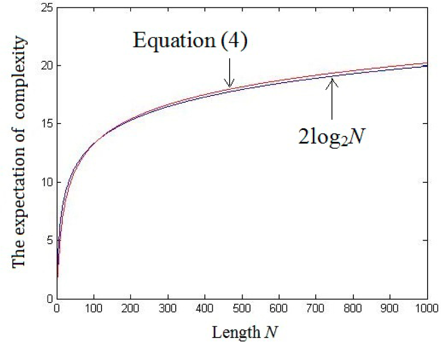
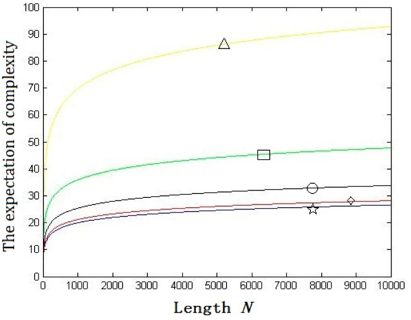
3. The Relationship between Nonlinear Complexity and Shannon’s Entropy

In this section, we will reveal the relationship between nonlinear complexity and Shannon’s entropy. From Figure 6 we know that the variance of nonlinear complexity is stable for a moderate large length N, thus the nonlinear complexity of a random binary sequence with length N approximately equals to its expectation. According to (6), the probabilities of “0” and “1” in random binary sequences are

$$p_1=\frac{1+\sqrt{2d-1}}{2},p_2=\frac{1-\sqrt{2d-1}}{2}$$

respectively. Here, $d=e^{\frac{-2\log N}{c}}$, and p₁ + p₂ = 1. Then, the function between Shannon’s entropy and nonlinear complexity is

$$\begin{array}{l}h=-{\displaystyle \sum _{i=1,2}{p}_i\log p_i}=-\frac{1+\sqrt{2d-1}}{2}\log \frac{1+\sqrt{2d-1}}{2}-\frac{1-\sqrt{2d-1}}{2}\log \frac{1-\sqrt{2d-1}}{2}\\ =\frac{1}{2}\log 2-\frac{1}{2}\log (1-d)-\frac{\sqrt{2d-1}}{2}\log \frac{1+\sqrt{2d-1}}{1-\sqrt{2d-1}}\end{array}$$

(13)

The relationship between nonlinear complexity and Shannon’s entropy is shown in Figure 7. As shown in Figure 7 we can see that the Shannon’s entropy has inverse correlation with nonlinear complexity.

Correspondingly, for a uniformly distributed random M—alphabets sequence, we can also establish the relationship between nonlinear complexity and Shannon’s entropy as

$$h=\frac{2\log N}{E(c(s))}$$

(14)

From (14) we can also have that the Shannon’s entropy is strictly monotonically decreased with nonlinear complexity.

4. Conclusions

In this paper, we mainly study on the nonlinear complexity of random sequences of memoryless source. The statistical properties of nonlinear complexity of random sequences, including probability distribution, expectation and variance are provided. Furthermore, we also establish its relationship to Shannon’s entropy. The result shows that these two measures are exactly opposite. In our future work, we will study the relationship between other complexity measures and probability (entropy) measure.

References

1. Kalouptsidis, N. Signal Processing Systems: Theory and Design; Wiley: New York, NY, USA, 1996. [Google Scholar]
2. Golomb, S.W. Shift Register Sequences; Holden-Day: San Francisco, CA, USA, 1967. [Google Scholar]
3. Wang, X.M.; Zhang, W.F.; Guo, W.; Zhang, J.S. Secure chaotic system with application to chaotic ciphers. Inf. Sci. 2013, 221, 555–570. [Google Scholar]
4. Menezes, A.J.; van Oorschot, P.C.; Vanstone, S.A. Handbook of applied cryptography; CRC Press: Boca Raton, FL, USA, 1996. [Google Scholar]
5. Stojanovski, T.; Kocarev, L. Chaos-based random number generators-part I: Analysis [cryptography]. IEEE Trans. Circ. Syst. I 2001, 48, 281–288. [Google Scholar]
6. Callegari, S.; Rovatti, R.; Setti, G. Embeddable ADC-based true random number generator for cryptographic applications exploiting nonlinear signal processing and chaos. IEEE Trans. Signal Process. 2005, 53, 793–805. [Google Scholar]
7. Addabbo, T.; Alioto, M.; Fort, A.; Rocchi, S.; Vignoli, V. A feedback strategy to improve the entropy of a chaos-based random bit generator. IEEE Trans. Circ. Syst. I 2006, 53, 326–337. [Google Scholar]
8. Nejati, H.; Beirami, A.; Ali, W.H. Discrete-time chaotic-map truly random number generators: Design, implementation and variability analysis of the zigzag map. Analog Integr. Circuits Signal Process. 2012, 73, 363–374. [Google Scholar]
9. Beirami, A.; Nejati, H.; Ali, W.H. Zigzag map: A variability-aware discrete-time chaotic map truly random number generator. Electron. Lett. 2012, 48, 1537–1538. [Google Scholar]
10. Shannon, C.E.; Weaver, W. The Mathematical Theory of Communication; University of Illinois Press: Champaign, IL, USA, 1949. [Google Scholar]
11. Kohda, T.; Tsuneda, A. Statistics of chaotic binary sequences. IEEE Trans. Inf. Theory 1997, 43, 104–112. [Google Scholar]
12. Kodha, T.; Tsuneda, A.; Lawrance, A.J. Correlational properties of Chebyshev chaotic sequences. J. Time Ser. Anal. 2000, 21, 181–191. [Google Scholar]
13. Visweswariah, K.; Kulkarni, S.R.; Verdu, S. Source codes as random number generators. IEEE Trans. Inf. Theory 1998, 44, 462–471. [Google Scholar]
14. Beirami, A.; Nejati, H. A framework for investigating the performance of chaotic-map truly random number generators. IEEE Trans. Circ. Syst. II 2013, 60, 446–450. [Google Scholar]
15. Beirami, A.; Nejati, H.; Callegari, S. Fundamental performance limits of chaotic-map random number generators. Proceedings of 52nd Annual Allerton Conference on Communication, Control and Computing, Monticello, IL, USA, 1–3 October 2014; pp. 1126–1131.
16. Massey, J.L. Shift register synthesis and BCH decoding. IEEE Trans. Inf. Theory 1969, 15, 122–127. [Google Scholar]
17. Limniotis, K.; Kolokotronis, N.; Kalouptsidis, N. New results on the linear complexity of binary sequences. Proceedings of 2006 IEEE International Symposium on Information Theory, Seattle, WA, USA, 9–14 July 2006; pp. 2003–2007.
18. Erdmann, D.; Murphy, S. An approximate distribution for the maximum order complexity. Des. Codes Cryptogr. 1997, 10, 325–339. [Google Scholar]
19. Rizomiliotis, P.; Kalouptsidis, N. Results on the nonlinear span of binary sequences. IEEE Trans. Inf. Theory 2005, 51, 1555–1563. [Google Scholar]
20. Lempel, A.; Ziv, J. On the complexity of finite sequences. IEEE Trans. Inf. Theory 1976, 22, 75–81. [Google Scholar]
21. Ziv, J.; Lempel, A. A universal algorithm for sequential data compression. IEEE Trans. Inf. Theory 1977, 23, 337–343. [Google Scholar]
22. Hamano, K.; Yamamoto, H. A differential equation method to derive the formulas of the T-complexity and the LZ-complexity. Proceedings of 2009 IEEE international conference on Symposium on Information Theory, Seoul, Korea, 28 June–3 July 2009; pp. 625–629.
23. Jansen, C.J.A. The maximum order complexity of sequence ensembles. In Advances in Cryptology—Eurocrypt’91; Davies, D.W., Ed.; Springer: Berlin/Heidelberg, Germany, 1991; pp. 153–159. [Google Scholar]
24. Niederreiter, H.; Xing, C.P. Sequences with high nonlinear complexity. IEEE Trans. Inf. Theory 2014, 60, 6696–6701. [Google Scholar]
25. Limniotis, K.; Kolokotronis, N.; Kalouptsidis, N. On the nonlinear complexity and Lempel-Ziv complexity of finite length sequences. IEEE Trans. Inf. Theory 2007, 53, 4293–4302. [Google Scholar]
26. Jansen, C.J.A.; Boekee, D.E. The shortest feedback shift register that can generate a given sequence. In Advances Cryptology—CRYPTO’89; Brassard, G., Ed.; Springer: Berlin/Heidelberg, Germany, 1990; pp. 90–99. [Google Scholar]
27. Ebeling, W.; Steuer, R.; Titchener, M.R. Partition-based entropies of deterministic and stochastic maps. Stoch. Dyn. 2001, 1, 45–61. [Google Scholar]
28. Liu, L.F.; Miao, S.X.; Hu, H.P.; Deng, Y.S. On the eigenvalue and Shannon’s entropy of finite length random sequences. Complexity 2014. [Google Scholar] [CrossRef]
Figure 1. (a). The probability distribution of nonlinear complexity of random binary sequence with p = 0.3. (b). Enlargement of (a).
Entropy 17 01936f1
Figure 2. (a). The probability distribution of nonlinear complexity of random binary sequence with p = 0.5. (b). Enlargement of (a).
Entropy 17 01936f2
Figure 3. The comparison of expectation of nonlinear complexity—Equation (4) E ( c ( s N ) ) = l = 1 N l P ( c ( s N ) = l ) = l = 1 N l ( ( 1 1 2 l ) C N l + 1 2 ( 1 1 2 l 1 ) C N l + 2 2 ) (red line) and 2log2N line (blue line).
Entropy 17 01936f3
Figure 4. The error between the expectation of nonlinear complexity and 2log2N.
Entropy 17 01936f4
Figure 5. The expectation of nonlinear complexity profile with p = 0.5 (blue line with a star logo), p = 0.4 (red line with a diamond shaped logo), p = 0.3 (black line with a circular logo), p = 0.2 (green line with a square logo) and p = 0.1 (yellow line with a triangle logo), respectively.
Entropy 17 01936f5
Figure 6. The variance of nonlinear complexity of random binary sequence with p = 0.5.
Entropy 17 01936f6
Figure 7. The relationship between nonlinear complexity and Shannon’s entropy.
Entropy 17 01936f7