Article

Research on the Stability of Open Financial System

School of Economics and Management, Beijing University of Aeronautics & Astronautics, 37 Xueyuan Road, Haidian District, Beijing 100191,China
*
Author to whom correspondence should be addressed.
These authors contributed equally to this work.
Entropy 2015, 17(4), 1734-1754; https://doi.org/10.3390/e17041734
Submission received: 6 February 2015 / Revised: 19 March 2015 / Accepted: 24 March 2015 / Published: 27 March 2015
(This article belongs to the Special Issue Recent Advances in Chaos Theory and Complex Networks)

Abstract

:
We propose a new herd mechanism and embed it into an open financial market system, which allows traders to get in and out of the system based on some transition rates. Moreover, the novel mechanism can avoid the volatility disappearance when the population scale increases. There are three kinds of heterogeneous agents in the system: optimistic, pessimistic and fundamental. Interactions especially occur among three different groups of agents instead of two, which makes the artificial financial market more close to the real one. By the simulation results of this complex system, we can explain stylized facts like volatility clustering and find the key parameters of market bubbles and market collapses.

1. Introduction

Financial markets are complex dynamic systems. Large numbers of traders interact in financial markets, which creates a complex system of different agents’ interdependent interaction patterns. More and more researchers have grappled with the modeling of financial markets for the last few decades. Nevertheless, traditional modeling approaches based on the Efficient Market Hypothesis (EMH) cannot explain some empirical stylized facts, like fat tails of returns and volatility clusters.
The Interacting Agent Hypothesis (IAH) was proposed to explore the mechanism which leads to abnormal market fluctuations in financial markets. It mainly concerns two opinions different from EMH—heterogeneous and endogenous. First, the term heterogeneous means the market consists of agents with different characteristics, for instance, different moods, trading strategies, learning mechanisms; that is, the agents in the market have different levels of rationality. The rational traders’ arbitrage capacity is limited, which makes it difficult to drive the prices close enough to the fundamental value in a finite time horizon [1,2]. How rational traders get profits depends on the uncertain time for price reversal, so they will bear more risk if the reversal time is longer [3]. These risks mean rational agents cannot drive the less rational agents out of the market, on the contrary, if there are a highly proportion of less rational traders in the market their buying (or selling) of assets may lead to market bubbles (or collapses) that will make rational traders lose a lot of money, so in a way, less rational traders expel rational traders from the financial market. Thus, heterogeneous agents coexist in the market. Second, because of the heterogeneity, agents can interact with each other, for example, by exchanging information, or imitating others’ behavior. Then with the endogenous dynamics through one-to-one relationships, the stability of the market is not only governed by the exogenous news arrival process but also determined by the inside interactions among agents. These two hypotheses make the financial market more unpredictable, and the fluctuations maybe more violent. In a sense, it can better explain and simulate the stylized facts. Many behavioral approaches based on this interacting hypothesis have emerged over the past two decades.
The initial models based on the interacting mechanism were established by Kirman [4,5] and DeGrauwe et al. [6]. They described the interacting mechanism and use their models to simulate the random walk features of asset prices and exchange rates. The endogenous dynamics can be better reflected, and the models show that fluctuation changes are controlled by agents’ interactions. Their models are clearly different from a true random walk; some laws can be displayed through the internal interacting mechanism. It’s just like a man who is drunk might walk in a way that appears “random”, but in fact he could just be following a sine-like curve [7]. However, these models neglect the stylized facts of financial markets.
A lot of subsequent milestone works [810] investigated artificial markets with interacting heterogeneous agents. Unfortunately, these models are not used to explain the empirical stylized facts. Despite rare consideration of stylized facts, subsequent research has shown that the time series data produced by these interacting models can accord with the empirical data [3,11,12]. To reveal the volatility cluster puzzle and to continue improving the above models some works found the dynamics are characterized by endogenous changes in the population composition [3,11,13,14]. The strategy configuration within the population is also an important factor for the stability of the entire dynamic system. Then, the percolation models of statistical physics are adopted in the agent-based models [15]. With more methods utilized in these kinds of models, like statistical physics, non-linear chemical reaction, chaos theory, the stylized facts have been explained and duplicated better. After a series of researches an interesting phenomenon was noted—with an increasing number of market traders the stylized facts fade. Cont and Wagalath [16] proposed a quantitative framework to analyze the scenario where investors are distress selling in a large fund and point out that covariance between returns of two assets can be decomposed into a fundamental and a liquidity-dependent covariance. They present short selling as the realized correlation between assets and fund volatility. In other words, the stylized facts depend crucially on the system size (i.e., the number of agents) [14,17,18].
About this interesting problem we must highlight the work of Alfarano et al. [19]. They derived closed-form solutions for distribution of returns and their higher moments and other statistics based on a herd model [20]. Though analysis of the analytic solutions and simulation of the price process they infer under what conditions the model could mimic the stylized facts (fat tails and volatility cluster). Importantly, in order to explain the vanishing stylized facts they separate the notion of interaction into two parts—global interaction and local interaction, which exists in Horst models [21].
In this paper, we employ a novel method to reveal the stylized fact puzzles. Compared with the works mentioned above, there are three essential changes. First, the new herd mechanism can better reflect the real social herd behavior than the global interaction [5] and local interaction models [19]. Second, in the above research the agents’ interactions occur just among noise traders, namely herd behavior cannot happen between noise traders and fundamental traders. Herd behavior is a kind of psychological behavior so that it is universal in a heterogeneous market. Noise traders (optimistic and pessimistic) and fundamental traders can be switched in our model, which extends the traditional transformation into two groups to three groups. More realistic situations will be duplicated with the increasing complexity of the model. Last but not the least, the financial market must be an open system. The above discussions focus more on the system size along with vanishing stylized facts, but the system size is fixed and exogenous. It is a mistake to ignore the influence on the system stability of every agent when it enters the market. Thus, we cannot just suppose that system size is five hundred or fifty thousand or infinite, the change of real market size is continuous. The discrete assumption will ignore the impact on the volatility from the microscopic changes which are really important in financial markets. Our model is an open system and agents can pass in and out based on some different conditions. Combining the above three points—new herd mechanism, multiple-transformation and open system—we will analyse our model in two aspects. From the micro point of view, Langevin equations are used to simulate the price process (and return process) and mimic the bear (or bull) market. Especially we can find the timing when the volatility will appear and the characteristics of market fluctuation. Most importantly, this model can explain the puzzle of system size in a more reasonable way and overcome the disappearance of volatility. Furthermore, we point out under what specific market conditions (specific parameters) stylized facts will disappear (vanishing volatility). From the macro point of view, differential equations are employed to measure the stability of the system, get the distributions of different groups of agents and describe the evolution process of the system. The paper is organized as follows: in Section 2 we describe the new herd mechanism. Section 3 elaborates the specific description of the open system in a financial market. The micro and macro analysis will be presented in Sections 4 and 5, respectively. Finally, we summarize this paper in Section 6.

2. New Herd Mechanism

In this section, we will propose a new herd mechanism, and to better understand how it works, we need to review the mechanism of the ant model proposed by Kirman [5]. For two food resources, a majority of the ant population crowds in one source, after a while, most of them transfer to another one which is almost in no favor just now. The number of ants of both sides seems reversed, and every once in a while this phenomenon occurs. There are two reasons contributing to this ant mechanism. One is pairwise interaction and another is an autonomous switching [5,19]. The pairwise interaction means every two ants can meet each other at a time, then exchange of information, and whether they are following others or not depends on the return of previous interactions, and we assume that it’s impossible to have multiple meetings, so only one ant may switch at one time. Another important assumption is the lack of memory of the ants to guarantee the population dynamics follow a Markov process. The total number of agents is N, the number of agents in one source (state 1) is denoted by n, where n ∈{0, 1,…, N},obviously, the number of agents in the opposite source (state 2) is Nn. We known that three situations may happen in one pairwise interaction, n′ = n ±1 or recruitment fails (n′ = n). According to the recruitment mechanism the transition rates is given by:
ω ( n n + 1 ) = ( 1 n N ) ( ε + β n N ) ω ( n n 1 ) = n N ( ε + β ( 1 n N ) )
Here ε represents random switching, and the parameter β measures the strength of the influence of the companions (the herd mechanism coefficient). Then we can get the probabilities of transit from number n at time t to number n′ at time t + Δt. The Markovian conditional probabilities are denoted by ρ(n′,t + Δt n,t) =ω(nn′)Δt. It is clearly that the formalization of the transition rate includes two parts, the former part is a fraction of the population; the latter part is the strength of the herd effect. More concretely, the switches between two states are governed by one state’s density multiplied by the attraction strength of another state.
Using the Langevin equation to simulate Kirman’s transition rate in financial markets, Alfarano et al. [19] point out that the volatility vanished if the system size gradually expanded (N →∞). That’s because the transition rate depends on the term ο(1/N), which is called “local” nature. This result, obviously, is not consistent with the actual financial markets. To fix this problem, the transition rate is modified in a non-local way, which is shown as Equation (2):
ω ( n n + 1 ) = ( N n ) ( ε + β n ) ω ( n n 1 ) = n ( ε + β ( N n ) )
The fraction term is replaced by an integer term. The significant difference between these two transition rates is what the transition rate should depend on, the fraction of agents in the alternative states or the overall number of such agents. Let us reevaluate the merits and drawbacks of these two transition rates. The transitions’ dependence on the overall fractions of groups (local) will lose all interesting features when the number of agents is enormous. On the contrary, the transitions’ dependence on the overall number of agents (non-local) can avoid these problems. On the other hand, considering the real situation what is the exact mechanism of the herd behavior, local or non-local? Now, we will propose a new perspective about herd mechanism based on a psychology experiment [22]. In the experiment, psychologists arrange five people standing in an elevator; back to the door (normal people usually face the door). A few minutes later a man enters the elevator, standing face to the door. But quickly he was aware of something strange and turned round and followed the others. After many experiments psychologists always got the same result. Certainly, the herd mechanism has worked here. Analyzing the principle behind the mechanism, we are conscious of the fact that people are influenced only by others who are around them. Despite the fact almost all people stand facing the door in elevators, the people who can really impact you are those who are standing in the same elevator with you. So how many people are around you (around you means you can observe each other and they can directly influence your decision) is the key point about how powerful the herd mechanism is rather than the overall number agents in the system. i.e., there may be a thousand students in your college, nevertheless, you may be familiar with only a hundred of them. Obviously if you want to decide what kind of sport to play it will just depend on what is majority of your friends want to play, instead of other nine hundred who you may never know. Thus, the herd behavior is a local mechanism in financial markets.
According to this new herd mechanism we can derive a new transition rate. Foremost, suppose that the number of agents’ friends (people who are around an agent) is denoted by m. Additionally, the number m will increase if more and more participants enter the system. m = m ¯ ln N , m ¯ N. m ¯ is a fixed minimum value of number of agents’ friends. Assuming that different states of agents have the same proportions both in m and N. Taking state 1 as example, the overall number of agents in state 1 is n, so that in m the number of agents in state 1 is m(n/N). Ultimately, based on the new herd behavior the transition rate is as follows:
ω ( n n + 1 ) = ( N n ) ( β m n N ) = ( N n ) ( β m ¯ n ln N N ) ω ( n n 1 ) = n ( β m N n N ) = n ( β m ¯ ( N n ) ln N N )
Here β is not fixed, different states have different herd strengths, and the value of β sometimes changes according to circumstances. i.e., speculators are more easily following the optimistic mood in a bull market than the pessimistic one and vice versa in a bear market. In the following work, we build up an open transfer system that depends on this herd dynamics and can explain the volatility in many aspects.

3. Open System in Financial Market

We set up an open system in a financial framework based on the novel herd dynamical mechanism. The system (or financial market) is populated by a variable number of agents N. Two groups of agents, noise traders and fundamental traders, occupy the market. According to the different speculation sentiments, noise traders are separated into two parts: optimistic and pessimistic, respectively, who expect the price to increase or decrease in the future. We interpret optimistic, pessimistic and fundamental as groups 1, 2 and 3. The number of agents in the different groups will be denoted by n i , n i { 0 , 1 , , N } , i n i = N , i = 1 , 2 , 3.The stochastic evolution of the system is governed by transfer between the three groups.
The system’s switching pattern is described in Figure 1. First, among the noise traders, optimists and pessimists can, unconditionally, interconvert (process (2) and (3)). Second, we define noise traders are less rational because they just follow the past one period price. After a long time observing other fundamental traders’ strategies, noise traders may follow them (process (5) and (6)). However, the herd strength of fundamental traders is far less than the strength between optimists and pessimists. Here assuming that there is a cost C for fundamental traders to collect information. If the cost is big they have no motivation to abandon the preceding cost switching to noise traders. Finally, the financial market is an open system, it allows anyone to get in and out of the financial market, but we stipulate that when a new trader gets into the system, he has no information about the market so he must be a noise trader (process (1) and (4)). On the contrary, only fundamental agents can realize their return is less than the cost to escape from the market (process (7)). These above seven processes constitute an open system.
We embed the open dynamic system into a financial framework. Optimists are assumed to buy additional units of the asset while pessimists sell the same units, and this certain number can be considered as the average transaction volume of noise traders, denoted by Tn. The excess demand of noise traders depends on the D-value (DV = x1x2, where xi = (ni/N) is the density of traders) between optimists and pessimists. If the D-value is zero that means there is no excess demand and if it is positive or negative (the same as excess demand) it amounts to the optimistic or pessimistic majorities. Therefore, noise traders’ excess demand is EDn = (n1 + n2)Tn(x1x2).
Furthermore, fundamental traders decide buy or sell based on whether the current price p is below or above the fundamental value p′f they evaluated. It is traditionally assumed in finance models that the fundamental value pf is known with certainty [23]. Although pf is an exogenous constant, it’s too difficult for agents to collect all the information about the market, especially, if the information contains noise, so to get the precise fundamental value is merely impossible. If only fundamental agents occupy the market without any noise (n3 = N), the fundamental value they expected is unbiased (p′f = pf). Actually, the accuracy of the evaluated price is improved as the fraction of fundamental traders increases. A damping function p f = p f + B e a x 3 sin ( λ x 3 + ϕ ) can depict this well. Adjusting the parameters B, a, λ, φ one can imitate different evaluate paths. Assuming that their average trading volume is Tf and their excess demand reacts on relative deviations between p and p f, this amounts to E D f = n 3 T f ln ( p f p ).
Within a Walrasian scenario, the equilibrium price changes would depend on overall excess demand E D = E D f + E D n, the relative price adjustment mechanism is:
1 p d p d t = γ E D = γ ( n 3 T f ln ( p f p ) + ( n 1 + n 2 ) T n ( x 1 x 2 ) )
with γ being the price adjustment speed.
Setting n 3 T f / ( n 1 + n 2 ) T n = 1, and the market instantaneous clearing (γ →∞), then the equilibrium price is derived by ED= EDf +EDn = 0.
ln ( p f p ) = ( n 1 + n 2 ) T n ( x 1 x 2 ) n 3 T f = ( x 1 x 2 ) p = p f e x 1 x 2 p = ( p f + B e a x 3 sin ( b x 3 + ϕ ) ) e x 1 x 2
The equilibrium price is driven both by the accuracy of fundamental traders’ fundamental value forecasting and the average mood of noise traders. The densities of the three groups of agents are important here and they are all stochastic processes depending on transition rates. This clearly proves that an agent switching among the three groups is the motivating power of this open system’s stochastic dynamics. The agents’ distribution determines the dynamic properties of the system. However, we are more interested in return volatility than prices. From the price process returns are computed using Equation (6):
r ( t + τ ) = ln p ( t + τ ) ln p
A simple open financial market system with heterogeneous interacting agents is constructed. We will analyze this framework at both the micro and macro levels. We can simulate the transition process under many different situations and find the reason for the existence of volatility clusters at a micro level. We will employ differential equations to depict the stability of the system at a macro level.

4. Micro Analysis

From the micro perspective, we expect to get the price process (or return process) under different parameters. Then, we hope to point out why these situations happen and to what extent they can reflect the real market. We employ some methods of statistical physics and non-linear chemistry to do approximations. First, we approximate the structure of the model and get the analysis expression of the population switching process. Second, we employ the analysis solution in the financial market and then simulate the price and return process.

4.1. Analysis Methods
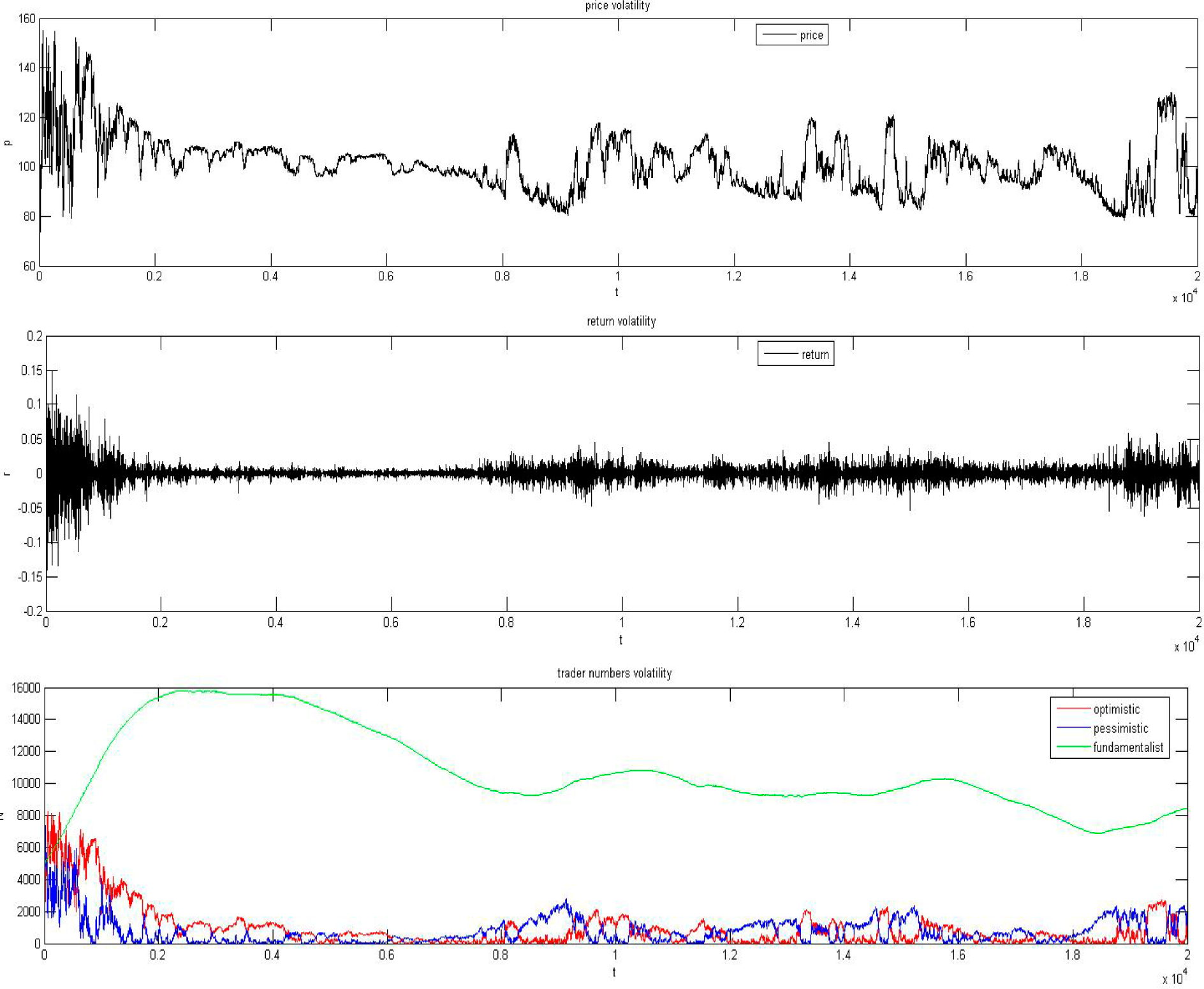
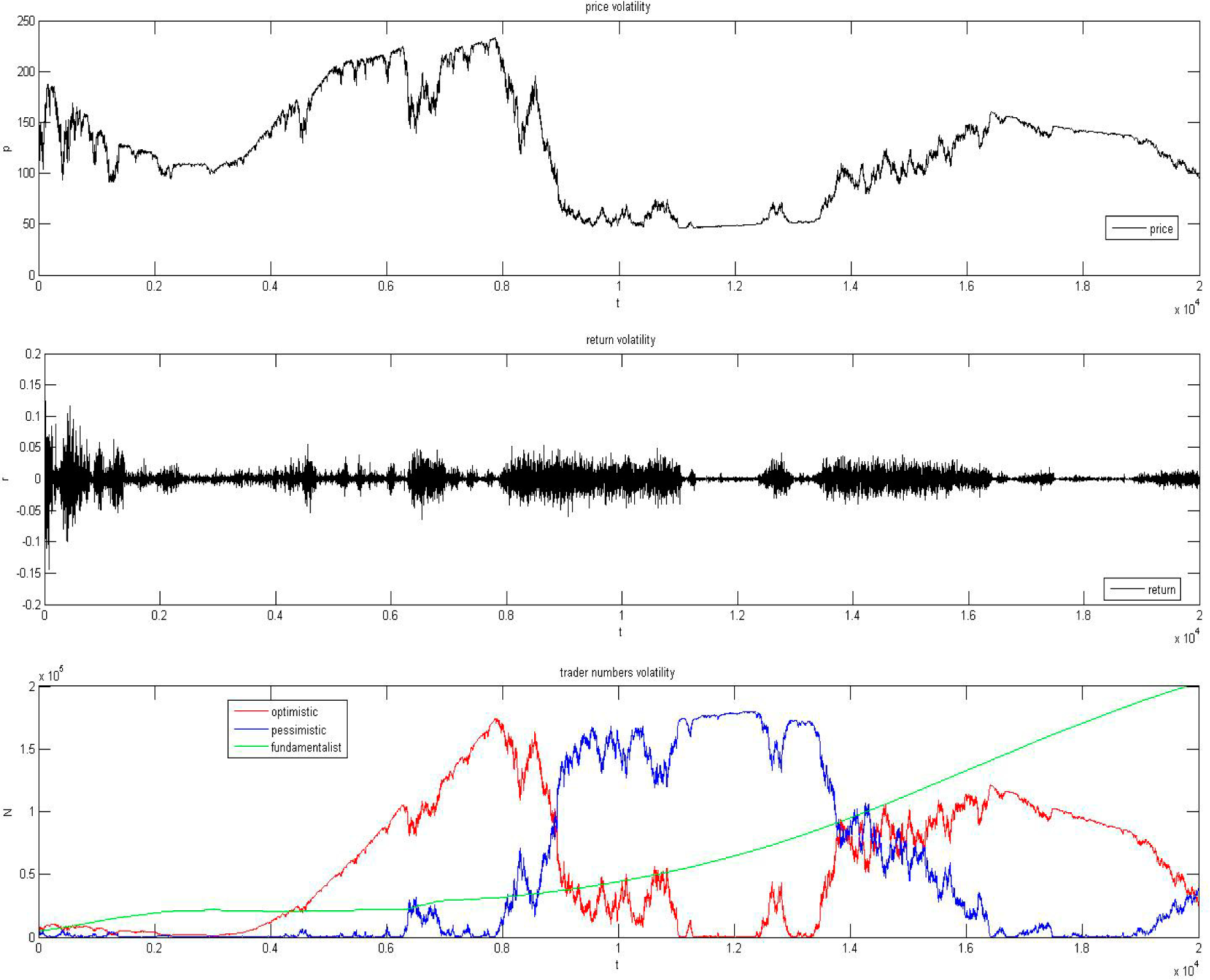
We denote the dynamical state of this system by X ( t ) ( X 1 ( t ) , X 2 ( t ) , X 3 ( t ) ), where Xi(t) means the number of agents of group i (ni) in the system at time t. X(t) is a random variable. In order to describe the evolution of X(t), we must make clearly the transition rate ωj for each interaction channel (or transition process).
According to the herd mechanism described in Section 2 we can define the transition rates of the system’s seven processes as follows:
ω 1 ( A n 1 ) = β 1 m ¯ n 1 N ln N ω 2 ( n 1 n 2 ) = n 1 ( β 2 m ¯ n 2 N ln N ) ω 3 ( n 2 n 1 ) = n 2 ( β 3 m ¯ n 1 N ln N ) ω 4 ( A n 2 ) = β 4 m ¯ n 2 N ln N ω 5 ( n 1 n 3 ) = n 1 ( β 5 m ¯ n 3 N ln N ) ω 6 ( n 2 n 3 ) = n 2 ( β 6 m ¯ n 3 N ln N ) ω 7 ( n 3 A ) = β 7
Agents outside of the system are denoted by A. We cannot evaluate the certain size of the external system, but we know only one agent switches every time. Then in order to simplify the transition rate of process one and four, we use one to multiply the herd term. In the process (7), the reason why fundamental traders escape from the market is unconcerned with the herd effect, so a parameter β7 is set as the transition rate. The different β here means the strength of herd effect in different groups is a different value. These transition probabilities make up a Markovian stochastic process which is called the “one-step processes”.
The transition rate ωj and the state-change vector νj, whose i-th component is defined by νji means the change in the number of ni produced by one j-th reaction (j = 1,…,7; i = 1,2,3), together completely explicate the j-th transition process. Here, on the basis of the open system, we can easily get the matrix ν as follows:
ν = ( ν 11 ν 12 ν 13 ν 21 ν 22 ν 23 ν 31 ν 32 ν 33 ν 41 ν 42 ν 43 ν 51 ν 52 ν 53 ν 61 ν 62 ν 63 ν 71 ν 72 ν 73 ) = ( 1 0 0 1 1 0 1 1 0 0 1 0 1 0 1 0 1 1 0 0 1 ) .
Under the above conditions, we derive a multivariate Langevin equation (stochastic difference equation) to approximate the stochastic process [24]. We show the details of the derivation of the Langevin equation in Appendix A.1. The multivariate Langevin equation is given by Equation (9):
X i ( t + d t ) = X i ( t ) + j ν j i ω j ( X ( t ) ) d t + j ν j i ω j 1 / 2 ( X ( t ) ) η j ( t ) ( d t ) 1 / 2 ( i = 1 , 2 , 3 )
η j ( t ) obeys a normal distribution with mean 0 and variance 1. With an appropriate time scale Δt, we obtain three equations to describe the system:
X 1 ( t + Δ t ) = X 1 ( t ) + m ¯ ln N N ( β 1 X 1 ( t ) ( β 2 β 3 ) X 1 ( t ) X 2 ( t ) β 5 X 1 ( t ) X 3 ( t ) ) Δ t + m ¯ ln N N ( β 1 X 1 ( t ) η 1 ( t ) β 2 X 1 ( t ) X 2 ( t ) η 2 ( t ) + β 3 X 1 ( t ) X 2 ( t ) η 3 ( t ) β 5 X 1 ( t ) X 3 ( t ) η 5 ( t ) ) ( Δ t ) 1 / 2
X 2 ( t + Δ t ) = X 2 ( t ) + m ¯ ln N N ( β 4 X 2 ( t ) + ( β 2 β 3 ) X 1 ( t ) X 2 ( t ) β 6 X 2 ( t ) X 3 ( t ) ) Δ t + m ¯ ln N N ( β 4 X 2 ( t ) η 4 ( t ) + β 2 X 1 ( t ) X 2 ( t ) η 2 ( t ) β 3 X 1 ( t ) X 2 ( t ) η 3 ( t ) β 6 X 2 ( t ) X 3 ( t ) η 6 ( t ) ) ( Δ t ) 1 / 2
X 3 ( t + Δ t ) = X 3 ( t ) + ( m ¯ ln N N ( β 5 X 1 ( t ) X 3 ( t ) + β 6 X 2 ( t ) X 3 ( t ) ) β 7 ) Δ t + ( m ¯ ln N N ( β 5 X 1 ( t ) X 3 ( t ) η 5 ( t ) + β 6 X 2 ( t ) X 3 ( t ) η 6 ( t ) ) β 7 η 7 ( t ) ) ( Δ t ) 1 / 2
Equations (10)(12) describe the dynamical evolutionary process of the open financial market. The next subsection will show the simulation results based on the above three equations.

4.2. Simulation

The parameter β is a variable to measure the strength of the herd effect and changes with the market’s mood. The mechanism of this change involves the fluctuation of people’s mood in particular cases and the observation and estimation of market performance under different moods. We know that when positive news is announced in a normal fluctuating market, traders want additional assets, but in the initial stage the volumes of the additional assets are not much. The excess demand, importantly, is increased, so that price is rising. The small price growth activates the mechanism of our model. The model contains irrational agents and rational agents, but the so-called irrational agents are not totally careless about the market information. They pay attention to the price trends and make profits as the goal. During two periods, optimistic traders will profit and pessimistic traders will lose when the market price is rising. So a proportion of pessimistic traders will change their state to optimistic for profit, at the same time, the increasing numbers of optimistic traders push the price up further (the caveat here, is that because the switch from pessimistic to optimistic is due to the rising price, and the price growth depends on the increasing numbers of optimistic traders, so that for pessimistic traders, to some extent, to observe the price is to follow the optimistic traders. It seems that the herd mechanism we introduced in Section 2 can better description this kind of behavior). This feedback mechanism creates a bull market. In the bull market, obviously, almost all new traders hold the optimistic attitude ( β 1 β 4). Furthermore, less optimistic traders will switch to fundamental traders ( β 6 β 5). Vice versa, the market collapse is unavoidable if negative news quickly spreads in the financial market.
Based on the above analysis, we can do a series of simulations (by adjusting the parameters β in different periods) with the Langevin equations to approximate the real financial market, and find out how much does the herd behavior impacts the financial market. Especially, we hope to find out the conditions under which volatility clustering will occur.
In the simulation, the time horizon is t = 20,000, initial number of population is n1 = n2 = n3 = 5000, initial price and fundamental price is p0 = pf = 100. The parameters are constant and symmetry, the herd parameters between noise traders are the same (β2, β3), besides the parameters to get into the market (β1, β4) and transfer from noise traders to fundamental traders (β5, β6) are all equal. In this symmetric stochastic case, we find noise traders will nearly be expelled from the market after a series self-oscillations. Subsequently, after a period, noise traders reappear, but only in a small amount. Then noise traders switch regularly, fundamental traders undergo periodic fluctuations, and the total number of the population has no significant changes, and the market tends to stable (see Figure 2).
The same process is also reflected in the price and return. Price fluctuations and return volatility clusters occur when the traders switch between each other. Furthermore, when the market tends to be stable the price fluctuates around the fundamental price with small amplitude and the return volatility is maintained in a certain range. We regard this simulation as a baseline and do a little adjustment in the simulation so it can better simulate bull and bear markets (bubbles and collapse). For Figure 3, we divide the time horizon into three parts, t ≤ 3000, 3000 < t ≤ 8000, 8000 < t, when t ≤ 3000, when t ≤ 3000 the parameter setting as the same as simulation of Figure 1. For part two, 3000 < t ≤ 8000, we assume that the market sends a positive information, it does not matter whether private or public information, as long as it can guarantee the market optimism (vice versa, for negative information). In this time horizon, we increase β1 and decrease β5, β7, which causes the market to expand in that more people rush into the market at the same time and less investors leave the market. Most traders are optimistic, they want more market share to make money, the excess demand becomes large, and under this circumstance no one is willing to be a conservative fundamental trader. As we can see in the traders evolution picture, optimistic traders undergo explosive growth and dominate the market, meanwhile, observing the price evolution picture and return evolution picture, the rapidly rising price leads to a bubble. However, return volatility is not obvious, and that is why traders cannot realize their over- optimistic state (over-confidence), and prosperity breeds a collapse. In the last part the basic parameter setting is as same as part one (parameter symmetry), only that we decrease β5, β6 to recover the market, increase β7 to eliminate the traders who accessed the market in a fanaticism time (part two).
The herd mechanism does have a significant influence in this part, as the amount of optimistic and pessimistic traders is reversed. The price plummets to an all-time low, the market collapses and the bubble is broken. Especially, the volatility cluster happens when the traders switch between each other. Finally, the amounts of traders fall back to the initial number, and prices return to the fundamental price. Changing the parameter setting can mimic many market situations, and the herd effect is significant, and the open market determines when the market can freely expand or shrink.

5. Macro Analysis

5.1. Analysis Methods

In this section, we concentrate on macroscopic properties instead of specific price dynamics processes. In macro analysis one may ignore some micro stochastic force disturbances to the system, owing to the offset between different noises. On the contrary, we can consider more macroscopic properties like stability, evolutionary trends, and population distributions. For this open system, it’s almost impossible to get an analytical solution for the distribution because switching between three groups with free access is much more complicated than the closed system with only two groups. Nevertheless, we also use a method of chemical chaos to construct the master equation, and finally obtain the differential equations. Many macro properties can be discovered from these differential equations. Note that in this open system consists of many collection of interacting jump processes with state-coherence, and applying the master equation can let us make clear the fluctuation of the distribution function. Here we invoke the birth-death master equation as follows:
d P ( X i , t ) d t = j [ ω j ( { X i ν j i } { X i } ) P ( { X i ν j i } , t ) ω j ( { X i } { X i + ν j i } ) P ( { X i } , t ) ]
In principle, as long as we can determine the transition rates of each switching step in unit time, the master equation can be determined, and after solving the equation we can get the distribution function P(Xi, t) (in this model the distribution function is described by differential equations). The transition rates are still based on the new herd mechanism but it will be more specific under this analysis pattern. We concentrate on the all changes that may affect the original integrated state (X1, X2, X3) ≡ (n1, n2, n3). For example, focusing on the interaction process (2), one transition rate ω1 (n1n2) can completely express it. However, considering all the flux possibilities that can influence the initial states, we divide the process (2) into two situations. Situation 1, (n1 + 1, n2 − 1)→(n1, n2), Situation 2, (n1, n2)→(n1 + 1, n2 − 1). These two situations can, comprehensively, describe the effect from process (2) to the original states, and measure the fluctuation. In order to get the distribution function we first rewrite the transition rates based on the new herd mechanism and considering the overall states:
ω 11 [ ( n 1 1 , n 2 , n 3 ) ( n 1 , n 2 , n 3 ) ] = β 1 m ¯ ln N ( n 1 1 ) N ω 12 [ ( n 1 , n 2 , n 3 ) ( n 1 + 1 , n 2 , n 3 ) ] = β 1 m ¯ ln N n 1 N ω 21 [ ( n 1 + 1 , n 2 1 , n 3 ) ( n 1 , n 2 , n 3 ) ] = β 2 m ¯ ln N ( n 1 + 1 ) ( n 2 1 N ) ω 22 [ ( n 1 , n 2 , n 3 ) ( n 1 1 , n 2 + 1 , n 3 ) ] = β 2 m ¯ ln N ( n 1 ) ( n 2 N ) ω 31 [ ( n 1 1 , n 2 + 1 , n 3 ) ( n 1 , n 2 , n 3 ) ] = β 3 m ¯ ln N ( n 2 + 1 ) ( n 1 1 N ) ω 32 [ ( n 1 , n 2 , n 3 ) ( n 1 + 1 , n 2 1 , n 3 ) ] = β 3 m ¯ ln N ( n 2 ) ( n 1 N ) ω 41 [ ( n 1 , n 2 1 , n 3 ) ( n 1 , n 2 , n 3 ) ] = β 4 m ¯ ln N ( n 2 1 ) N ω 42 [ ( n 1 , n 2 , n 3 ) ( n 1 , n 2 + 1 , n 3 ) ] = β 4 m ¯ ln N n 2 N ω 51 [ ( n 1 + 1 , n 2 , n 3 1 ) ( n 1 , n 2 , n 3 ) ] = β 5 m ¯ ln N ( n 1 + 1 ) ( n 3 1 N ) ω 52 [ ( n 1 , n 2 , n 3 ) ( n 1 1 , n 2 , n 3 + 1 ) ] = β 5 m ¯ ln N ( n 1 ) ( n 3 N ) ω 61 [ ( n 1 , n 2 + 1 , n 3 1 ) ( n 1 , n 2 , n 3 ) ] = β 6 m ¯ ln N ( n 2 + 1 ) ( n 3 1 N ) ω 62 [ ( n 1 , n 2 , n 3 ) ( n 1 , n 2 1 , n 3 + 1 ) ] = β 6 m ¯ ln N ( n 2 ) ( n 3 N ) ω 71 [ ( n 1 , n 2 , n 3 + 1 ) ( n 1 , n 2 , n 3 ) ] = β 7 ( n 3 + 1 ) ω 72 [ ( n 1 , n 2 , n 3 ) ( n 1 , n 2 , n 3 1 ) ] = β 7 n 3
ω j k means j-th process in situation k. Here we revise the transition rate in process (7) from exogenous to endogenous. Assuming that outside agents’ herd strength equals one, this assumption can simplified calculation and not lose generality. Putting these transition rates into Equation (13), we obtain following master equation:
P ( n 1 , n 2 , n 3 , t ) t = [ β 1 m ¯ ln N n 1 1 N ] P ( n 1 1 , n 2 , n 3 , t ) [ β 1 m ¯ ln N n 1 N ] P ( n 1 , n 2 , n 3 , t ) + [ β 2 m ¯ ln N ( n 1 + 1 ) ( n 2 1 ) N ] P ( n 1 + 1 , n 2 1 , n 3 , t ) [ β 2 m ¯ ln N ( n 1 ) n 2 N ] P ( n 1 , n 2 , n 3 , t ) + [ β 3 m ¯ ln N ( n 2 + 1 ) ( n 1 1 ) N ] P ( n 1 1 , n 2 + 1 , n 3 , t ) [ β 3 m ¯ ln N ( n 2 ) n 1 N ] P ( n 1 , n 2 , n 3 , t ) + [ β 4 m ¯ ln N n 2 1 N ] P ( n 1 , n 2 1 , n 3 , t ) [ β 4 m ¯ ln N n 2 N ] P ( n 1 , n 2 , n 3 , t ) + [ β 5 m ¯ ln N ( n 1 + 1 ) ( n 3 1 ) N ] P ( n 1 + 1 , n 2 , n 3 1 , t ) [ β 5 m ¯ ln N ( n 1 ) n 3 N ] P ( n 1 , n 2 , n 3 , t ) + [ β 6 m ¯ ln N ( n 2 + 1 ) ( n 3 1 ) N ] P ( n 1 , n 2 + 1 , n 3 1 , t ) [ β 6 m ¯ ln N ( n 2 ) n 3 N ] P ( n 1 , n 2 , n 3 , t ) + [ β 7 ( n 3 + 1 ) ] P ( n 1 , n 2 , n 3 + 1 , t ) [ β 7 n 3 ] P ( n 1 , n 2 , n 3 , t )
Using the cumulative generating function expansion method to solve the master equation, we can get the density fluctuation for every group of agents formalized by differential equations. Then, we obtain the following ordinary differential equations (see Appendix A.2 for details):
{ d x 1 d t = ( β 3 β 2 ) m ¯ ln N ( x 1 x 2 ) β 5 m ¯ ln N ( x 1 x 3 ) d x 2 d t = ( β 2 β 3 ) m ¯ ln N ( x 1 x 2 ) β 6 m ¯ ln N ( x 2 x 3 ) d x 3 d t = β 7 x 3 + β 5 m ¯ ln N ( x 1 x 3 ) + β 6 m ¯ ln N ( x 2 x 3 )
Equation (16) contains both the mean value and the evolution of temporally dependent fluctuation. These partial differential equations can describe stabilities of the whole system as well as they performed well in describing chemical reactions. Through analyzing these partial differential equations, we can find out the evolutionary trend of the system which will give us a comprehensive understanding of the financial market.

5.2. Result Analysis

After solving the above partial differential equations, we can get more specific characteristics of the system, including the 3D-figure of the population ratio, and the distribution of each group (Figures 47). According to these results, we can further understand the stabilization and the structure of the three groups of traders switching model.
The results clearly show that all the three kind of agents present a bimodal distribution around different means. According to the Figure 5, the system is stable and independent with time. Combined with the findings in Section 4, these results can reflect well the properties of the real financial market—stable in the long-term but fluctuating occasionally, and those fluctuations are triggered by large and quick transfers among different kinds of agents.

6. Conclusions

The aim of this paper is to make the agent-based models more in line with the actual financial market, and to explain the stylized facts. To this end, we made three major breakthroughs and used many statistical methods to analyze the agent-based model from two aspects, the micro and macro. The insights are the following:
  • We successfully explained the relation between system size and fluctuation of financial market. Especially, through three improvements, we solved the puzzle that the loss of volatility depends on growing system size. The real market’s volatility never vanishes no matter how the market size is changing, because (1) the market is always an open system; (2) the herd behavior is effective among all traders. Besides, we redefined the herd mechanism from the behavior perspective which made the model more practical.
  • We have also pointed out the reasons why these financial anomalies, such as bubbles, collapses, and volatility clusters, happened. We derived the price process and return process by using some methods—multivariate Langevin equation and multivariate Fokker–Planck equation. Combining the analysis of these price and return processes which were derived based on our new herd mechanism we can clearly find out that which variables control the market volatility and the relationship between different variables, and all these variables have their actual meaning.
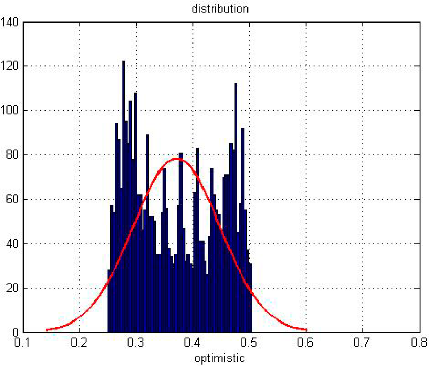
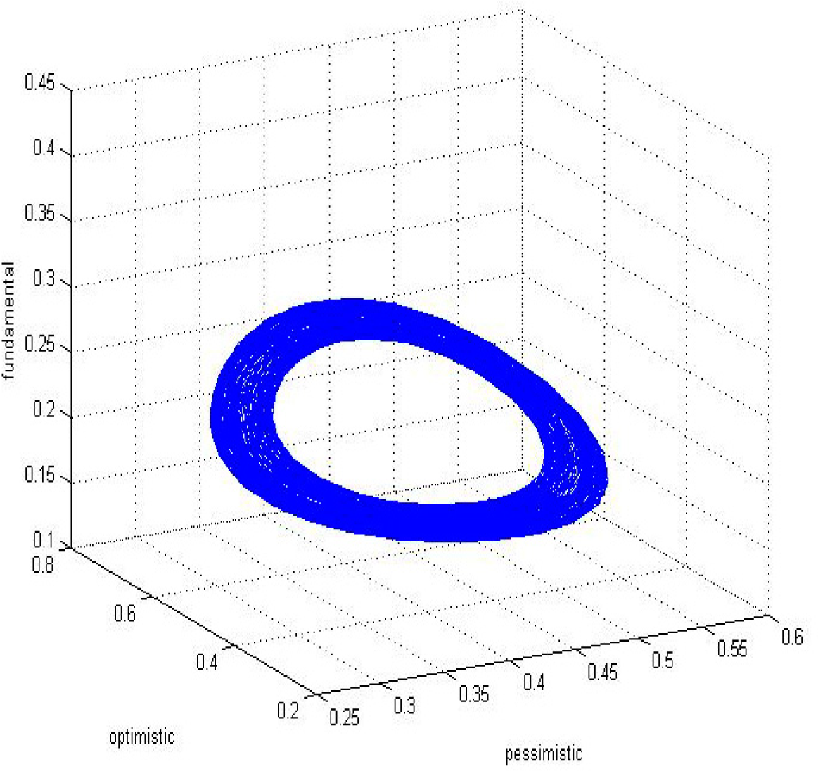
  • For the macro level, we employed a non-linear chemistry method to analyze our model and aim at the distribution of different agents with the changing time. The partial differential equations can perfectly describe the stability of the whole system and some statistical variables, such as mean and variance. These findings give us another way to explain the market volatility.

Appendix A

A.1. The multivariate Langevin equation

The Langevin approach is widely used in statistical physics and non-linear chemical reactions to mimic Brownian movement and some chemical reactions. The idea of the Langevin approach is to find an appropriate time interval, for which can approximate well the discrete variable (in this paper it is agents’ numbers) by a Gaussian. Here, we will use the multivariate Langevin equation to approximate the discrete process (Equation (7)); then get the evolution equations of the three groups of agents. In the following we sketch a derivation of the general form of the multivariate Langevin equation.
Let Kj (X (t), Δt), for any Δt>0, be the number of j-th reaction that occur in the subsequent time interval [t,t+ Δt]. Thus, the number of agents in the system at time [t+ Δt] can be written as follows:
X i ( t + Δ t ) = X i ( t ) + j K j ( X i ( t ) , Δ t ) ν j i ( i = 1 , 2 , 3 )
We impose the following two conditions to easily obtain an excellent approximation to the random variable K j ( X ( t ) , Δ t ).
Condition one: Letting Δ tto be small enough that the change in the state during [t,t+ Δt] will be so small that none of the transition rates changes appreciably. The transition rates then satisfy:
ω j ( X ( t ) ) ω j ( X ( t ) ) , t [ t , t + Δ t ] .
Under the definition of ω j, that each K j ( X ( t ) , Δ t ) will be a statistically independent Poisson random variable Ρ j ( ω j ( X ( t ) ) , Δ t ). So the effect of condition one is that approximate equation (A.1.1) will be:
X i ( t + Δ t ) = X i ( t ) + j Ρ j ( ω j ( X ( t ) ) , Δ t ) ν j i ( i = 1 , 2 , 3 )
Condition two: Require Δt to be large enough that the change number of agents of j-th reaction in [t,t+ Δt] be larger than 1, i.e.,:
Ρ j ( ω j ( X ( t ) ) , Δ t ) = ω j ( X ( t ) ) Δ t > 1
These two conditions seem to be contradictory, but there will be many practical circumstances in which these two conditions can be simultaneously satisfied. Condition two allows us to approximate each Poisson random variable P j ( ω j ( X ( t ) ) , Δ t ) by a normal random variable with the same mean and variance. Then we got the following result:
X i ( t + Δ t ) = X i ( t ) + j N j ( ω j ( X ( t ) ) Δ t , ω j ( X ( t ) ) Δ t ) ν j i ( i = 1 , 2 , 3 )
where N ( m , σ 2 ) denotes the normal random variable with mean m and variance σ 2.
The linear combination theorem for normal random variables:
N ( m , σ 2 ) = m + σ N ( 0 , 1 ) ,
Using this theorem, the equation will be:
X i ( t + Δ t ) = X i ( t ) + j ν j i ω j ( X ( t ) ) Δ t + j ν j i [ ω j ( X ( t ) ) Δ t ] 1 / 2 N j ( 0 , 1 ) ( i = 1 , 2 , 3 )
Let us denote the N j ( 0 , 1 ) to η j ( t ) as the random term, and Δt denote by d t. Finally, we get the general form of the multivariate Langevin equation:
X i ( t + d t ) = X i ( t ) + j ν j i ω j ( X ( t ) ) d t + j ν j i ω j 1 / 2 ( X ( t ) ) η j ( t ) ( d t ) 1 / 2 ( i = 1 , 2 , 3 )
This equation can well approximate the evolution of the three groups of traders. Then we can get the price and return process.

A.2. Cumulant Generating Function Expansion of the Master Equation

We use the cumulant generating function expansion method to solve the master equation. The form of the master equation is Equation (15). We define a generating function for the master equation:
F ( S n 1 , S n 2 , S n 3 , t ) = n 1 , n 2 , n 3 S n 1 n 1 S n 2 n 2 S n 3 n 3 P ( n 1 , n 2 , n 3 , t )
Here, | S n 1 | , | S n 2 | , | S n 3 | 1, when S n 1 = S n 2 = S n 3 = 1 can easily prove the relationship between each order partial derivative of the function F and the moments of the probability distribution function P:
F S n 1 ( 1 , 1 , 1 , t ) = n 1 , n 2 , n 3 n 1 P ( n 1 , n 2 , n 3 , t ) = n 1 F S n 2 ( 1 , 1 , 1 , t ) = n 1 , n 2 , n 3 n 2 P ( n 1 , n 2 , n 3 , t ) = n 2 F S n 3 ( 1 , 1 , 1 , t ) = n 1 , n 2 , n 3 n 3 P ( n 1 , n 2 , n 3 , t ) = n 3 F S n 1 ( 1 , 1 , 1 , t ) = n 1 , n 2 , n 3 n 1 ( n 1 1 ) P ( n 1 , n 2 , n 3 , t ) = n 1 2 n 1 F S n 2 ( 1 , 1 , 1 , t ) = n 1 , n 2 , n 3 n 2 ( n 2 1 ) P ( n 1 , n 2 , n 3 , t ) = n 2 2 n 2 F S n 3 ( 1 , 1 , 1 , t ) = n 1 , n 2 , n 3 n 3 ( n 3 1 ) P ( n 1 , n 2 , n 3 , t ) = n 3 2 n 3 F S n 1 S n 2 ( 1 , 1 , 1 , t ) = n 1 , n 2 , n 3 n 1 n 2 P ( n 1 , n 2 , n 3 , t ) = n 1 n 2 F S n 1 S n 3 ( 1 , 1 , 1 , t ) = n 1 , n 2 , n 3 n 1 n 3 P ( n 1 , n 2 , n 3 , t ) = n 1 n 3 F S n 2 S n 3 ( 1 , 1 , 1 , t ) = n 1 , n 2 , n 3 n 2 n 3 P ( n 1 , n 2 , n 3 , t ) = n 2 n 3
According to these comparison expressions, we can figure out the mean of every component and the evolution of fluctuation if only the generating function can be obtained. So, we multiply the S n 1 n 1 S n 2 n 2 S n 3 n 3 by both sides of the master equation, then do a summation of n1, n2, n3, after that can get a differential equation which the generating function F is satisfied with:
F ( S n 1 , S n 2 , S n 3 , t ) t = β 1 m ¯ ln N N ( S n 1 1 ) S n 1 F S n 1 ( S n 1 , S n 1 , S n 1 , t ) + β 2 m ¯ ln N N ( S n 2 S n 1 ) S n 2 F S n 1 S n 2 ( S n 1 , S n 2 , S n 3 , t ) + β 3 m ¯ ln N N ( S n 1 S n 2 ) S n 1 F S n 1 S n 2 ( S n 1 , S n 2 , S n 3 , t ) + β 4 m ¯ ln N N ( S n 2 1 ) S n 2 F S n 2 ( S n 1 , S n 2 , S n 3 , t ) + β 5 m ¯ ln N N ( S n 3 S n 1 ) S n 3 F S n 1 S n 3 ( S n 1 , S n 2 , S n 3 , t ) + β 6 m ¯ ln N N ( S n 3 S n 3 ) S n 3 F S n 2 S n 3 ( S n 1 , S n 2 , S n 3 , t ) + β 7 ( 1 S n 3 ) F S n 3 ( S n 1 , S n 2 , S n 3 , t )
In the above derivation process, we get the first term at the right side of the equal sign as follows:
n 1 , n 2 , n 3 β 1 m ¯ ln N N [ ( n 1 1 ) S n 1 n 1 S n 2 n 2 S n 3 n 3 P ( n 1 1 , n 2 , n 3 , t ) n 1 S n 1 n 1 S n 2 n 2 S n 3 n 3 P ( n 1 , n 2 , n 3 , t ) ] = n 1 , n 2 , n 3 β 1 m ¯ ln N N [ S n 1 ( n 1 1 ) S n 1 n 1 1 S n 2 n 2 S n 3 n 3 P ( n 1 1 , n 2 , n 3 , t ) n 1 S n 1 n 1 S n 2 n 2 S n 3 n 3 P ( n 1 , n 2 , n 3 , t ) ] = β 1 m ¯ ln N N ( S n 1 1 ) n 1 , n 2 , n 3 n 1 S n 1 n 1 S n 2 n 2 S n 3 n 3 P ( n 1 , n 2 , n 3 , t ) = β 1 m ¯ ln N N ( S n 1 1 ) S n 1 S n 1 F ( S n 1 , S n 2 , S n 3 , t )
The derivation of other six terms is the same. In this way, the complicated master equation has been reduced to a simpler differential equation. The equation can be simplified further. Therefore, we define a cumulant generating function ψ ( S ˜ n 1 , S ˜ n 2 , S ˜ n 3 , t ):
F ( S n 1 , S n 2 , S n 3 , t ) = e N ψ ( S ˜ n 1 , S ˜ n 2 , S ˜ n 3 , t ) S ˜ n 1 = S n 1 1 , S ˜ n 2 = S n 2 1 , S ˜ n 3 = S n 3 1
The Equation (A.2.3) substituted in Equation (A.2.2), can get a nonlinear partial differential equation which the cumulant generating function ψ is satisfied with:
N ψ t = ( β 1 m ¯ ln N ) S ˜ n 1 ( S ˜ n 1 + 1 ) ψ S ˜ n 1 + β 2 m ¯ ln N N ( S ˜ n 2 S ˜ n 1 ) ( S ˜ n 2 + 1 ) ( N ψ S ˜ n 1 S ˜ n 2 + N 2 ψ S ˜ n 1 ψ S ˜ n 2 ) + β 3 m ¯ ln N N ( S ˜ n 1 S ˜ n 2 ) ( S ˜ n 1 + 1 ) ( N ψ S ˜ n 1 S ˜ n 2 + N 2 ψ S ˜ n 1 ψ S ˜ n 2 ) + ( β 4 m ¯ ln N ) S ˜ n 2 ( S ˜ n 2 + 1 ) ψ S ˜ n 2 + β 5 m ¯ ln N N ( S ˜ n 3 S ˜ n 1 ) ( S ˜ n 3 + 1 ) ( N ψ S ˜ n 1 S ˜ n 3 + N 2 ψ S ˜ n 1 ψ S ˜ n 3 ) + β 6 m ¯ ln N N ( S ˜ n 3 S ˜ n 2 ) ( S ˜ n 3 + 1 ) ( N ψ S ˜ n 2 S ˜ n 3 + N 2 ψ S ˜ n 2 ψ S ˜ n 3 ) N β 7 S ˜ n 3 ψ S ˜ n 3
From the Equations (A.2.1) and (A.2.3) we obtain the following formulae:
ψ S ˜ n 1 ( 0 , 0 , 0 , t ) = n 1 N = x 1 ψ S ˜ n 3 ( 0 , 0 , 0 , t ) = n 2 N = x 2 ψ S ˜ n 3 ( 0 , 0 , 0 , t ) = n 3 N = x 3 ψ S ˜ n 1 ( 0 , 0 , 0 , t ) = n 1 2 n 1 2 n 1 N = δ n 1 2 n 1 N = b 11 ψ S ˜ n 2 ( 0 , 0 , 0 , t ) = n 2 2 n 2 2 n 2 N = δ n 2 2 n 2 N = b 22 ψ S ˜ n 3 ( 0 , 0 , 0 , t ) = n 3 2 n 3 2 n 3 N = δ n 3 2 n 3 N = b 33 ψ S ˜ n 1 S ˜ n 2 ( 0 , 0 , 0 , t ) = n 1 n 2 n 1 n 2 N = δ n 1 δ n 2 N = b 12 ψ S ˜ n 1 S ˜ n 3 ( 0 , 0 , 0 , t ) = n 1 n 3 n 1 n 3 N = δ n 1 δ n 3 N = b 13 ψ S ˜ n 2 S ˜ n 3 ( 0 , 0 , 0 , t ) = n 2 n 3 n 2 n 3 N = δ n 2 δ n 3 N = b 23
In addition, we do a linear approximation to the function ψ ( S ˜ n 1 , S ˜ n 2 , S ˜ n 3 , t ) at the point zero:
ψ ( S ˜ n 1 , S ˜ n 2 , S ˜ n 3 , t ) = x 1 S ˜ n 1 + x 2 S ˜ n 2 + x 3 S ˜ n 3 + 1 2 b 11 S ˜ n 1 2 + 1 2 b 22 S ˜ n 2 2 + 1 2 b 33 S ˜ n 3 2 + b 12 S ˜ n 1 S ˜ n 2 + b 13 S ˜ n 1 S ˜ n 3 + b 23 S ˜ n 2 S ˜ n 3
Then, we can get the ordinary differential equations after comparing the same power of S ˜ n 1 , S ˜ n 2 , S ˜ n 3in both Equations (A.2.4) and (A.2.5):
{ d x 1 d t = m ¯ ln N ( β 1 N x 1 β 2 N b 12 β 2 x 1 x 2 + β 3 N b 12 + β 3 x 1 x 2 β 5 N b 13 β 5 x 1 x 3 ) d x 2 d t = m ¯ ln N ( β 4 N x 2 + β 2 N b 12 + β 2 x 1 x 2 β 3 N b 12 β 3 x 1 x 2 β 6 N b 23 β 6 x 2 x 3 ) d x 3 d t = β 7 x 3 + m ¯ ln N ( β 5 N b 13 + β 5 x 1 x 3 + β 6 N b 23 + β 6 x 2 x 3 )
According to the L’Hospital rule with the expansion of the system’s scale ( N ), the term ln N N 0 ( lim N ln N N = lim N 1 N = 0 ). Finally, we get the reduced form of the ordinary differential Equation (16):
{ d x 1 d t = ( β 3 β 2 ) m ¯ ln N ( x 1 x 2 ) β 5 m ¯ ln N ( x 1 x 3 ) d x 2 d t = ( β 2 β 3 ) m ¯ ln N ( x 1 x 2 ) β 6 m ¯ ln N ( x 2 x 3 ) d x 3 d t = β 7 x 3 + β 5 m ¯ ln N ( x 1 x 3 ) + β 6 m ¯ ln N ( x 2 x 3 )

Acknowledgments

This work was supported by the National Natural Science Foundation of China (No.71171010).
PACS Codes: 89.75; 89.65.Gh

Author Contributions

This paper explains the relation between system size and fluctuation of financial market, and solves the puzzle that the loss of volatility depends on growing system size. We have also pointed out the reasons why these financial anomalies, such as bubbles, collapses, and volatility clusters, happened. Based on our new herd mechanism we can clearly find out that which variables control the market volatility and the relationship between different variables, and all these variables have their actual meaning. Finally, we describe the stability of the whole system and some statistical variables, such as mean and variance to explain the market volatility.

Conflicts of Interest

The authors declare no conflict of interest.

References

  1. Figlewski, S. Market “efficiency” in a market with heterogeneous information. J Polit. Econ. 1978, 86, 581–597. [Google Scholar]
  2. Shiller, R.J.; Fischer, S.; Friedman, B.M. Stock prices and social dynamics. Brook. Pap. Econ. Act. Rev. 1984, 2, 457–498. [Google Scholar]
  3. Lux, T.; Marchesi, M. Scaling and criticality in a stochastic multi-agent model of a financial market. Nature 1999, 397, 498–500. [Google Scholar]
  4. Kirman, A. Epidemics of opinion and speculative bubbles in financial markets. Money Financ. Mark. 1991, 354–368. [Google Scholar]
  5. Kirman, A. Ants, rationality, and recruitment. Q. J. Econ. 1993, 108, 137–156. [Google Scholar]
  6. De Grauwe, P.; Dewachter, H.; Embrechts, M.J. Exchange Rate Theory: Chaotic Models of Foreign Exchange Markets; Blackwell: Oxford, UK, 1993. [Google Scholar]
  7. Chen, S.H. Varieties of agents in agent-based computational economics: A historical and an interdisciplinary perspective. J. Econ. Dyn. Control 2012, 36, 1–25. [Google Scholar]
  8. Levy, M.; Levy, H.; Solomon, S. A microscopic model of the stock market: Cycles, booms, and crashes. Econ. Lett. 1994, 45, 103–111. [Google Scholar]
  9. Arifovic, J. The behaviour of the exchange rate in the genetic algorithm and experimental economies. J. Polit. Econ. 1996, 104, 510–541. [Google Scholar]
  10. Arthur, W.B.; Holland, J.H.; LeBaron, B.; Palmer, R.; Tayler, P. Asset pricing under endogenous expectations in an artificial stock market. Econ. Notes 1997, 26, 297–330. [Google Scholar]
  11. Lux, T.; Marchesi, M. Volatility clustering in financial markets: A microsimulation of interacting agents. Int. J. Theor. Appl. Financ 2000, 3, 675–702. [Google Scholar]
  12. Yang, H.J.; Gui, P.S. Study on the stability of an artificial stock option market based on bidirectional conduction. Entropy 2013, 15, 700–720. [Google Scholar]
  13. Giardina, I.; Bouchaud, J.-P. Bubbles, crashes and intermittency in agent based market models. Eur. Phys. J. B 2003, 31, 421–437. [Google Scholar]
  14. Lux, T.; Schornstein, S. Genetic learning as an explanation of stylized facts of foreign exchange markets. J. Math. Econ. 2005, 41, 169–196. [Google Scholar]
  15. Cont, R.; Bouchaud, J.P. Herd behaviour and aggregate fluctuations in financial markets. Macroecon. Dyn. 2000, 4, 170–196. [Google Scholar]
  16. Cont, R.; Wagalath, L. Running for the exit: distressed selling and endogenous correlation in financial markets. Math. Financ 2013, 23, 718–741. [Google Scholar]
  17. Egenter, E.; Lux, T.; Stauffer, D. Finite-size effects in Monte Carlo simulations of two stock market models. Physica A 1999, 268, 250–256. [Google Scholar]
  18. Challet, D.; Marsili, M. From minority game to the real markets. Phys. Rev. E 2004, 68, 168–176. [Google Scholar]
  19. Alfarano, S.; Lux, T.; Wagner, F. Time variation of higher moments in a financial market with heterogeneous agents: An analytical approach. J. Econ. Dyn. Control 2008, 32, 101–136. [Google Scholar] [Green Version]
  20. Kirman, A.; Teyssiere, G. Microeconomic models for long memory in the volatility of financial time series. Stud. Nonlinear Dyn. Econ. 2002, 5, 281–302. [Google Scholar]
  21. Horst, U. Financial price fluctuations in a stock market model with many interacting agents. Econ. Theory 2004, 25, 917–932. [Google Scholar]
  22. Sugiman, T.; Misumi, J. Development of a new evacuation method for emergencies: Control of collective behavior by emergent small group. J. Appl. Psychol 1998, 73, 3–10. [Google Scholar]
  23. De Grauwe, P.; Kaltwasser, P.R. Animal spirits in the foreign exchange market. J. Econ. Dyn. Control 2012, 36, 1176–1192. [Google Scholar]
  24. Gillespie, D.T. The chemical Langevin equation. J. Chem. Phys 2000, 113, 297–306. [Google Scholar]
Figure 1. Interaction agents of an open financial market.
Entropy 17 01734f1
Figure 2. Normal financial market (β1 = 1, β2 = 5, β3 = 5, β4 = 1, β5 = 0.00025, β6 = 0.00025, β7 = 3).
Entropy 17 01734f2
Figure 3. Market conditions shift from bull to bear cycles. (t ≤ 3000; β1 = 1, β2 = 5, β3 = 5, β4 = 1, β5 = 0.00025, β6 = 0.00025, β7 = 3. 3000 ˂ t ≤ 8000; β1 = 5, β2 = 5, β3 = 5, β4 = 1, β5 = 0.00001, β6 = 0.00003, β7 = 2. 8000 ˂ t; β1 = 1, β2 = 5, β3 = 5, β4 = 1, β5 = 0.00003, β6 = 0.00003, β7 = 5).
Entropy 17 01734f3
Figure 4. 3D-figure of the population ratio.
Entropy 17 01734f4
Figure 5. Distribution figure of optimistic traders.
Entropy 17 01734f5
Figure 6. Distribution figure of pessimistic traders.
Entropy 17 01734f6
Figure 7. Distribution figure of fundamental traders.
Entropy 17 01734f7

