1. Introduction
Mutualisms,
i.e., interactions between two species in which both benefit from the association, have been essential in the evolutionary diversification of life and are fundamental to preserve nature’s biodiversity [
1,
2]. Without mutualism, the biosphere would be entirely different. For instance, approximately 90% of flowering plants are pollinated by animals [
3], mainly by pollinator insects. In this mutualistic relationship, the pollinator obtains food (nectar), inadvertently picks up pollen and moves on to the next flower, allowing plants to reproduce.
However, the study of mutualisms as a non-trivial biological phenomena is a recent development in biology relative to the mainstream or Newtonian ecology [
1], based on antagonistic interspecific interactions (e.g., competition, predation). Antagonistic interactions have received much more attention than mutualistic ones, because mutualistic interactions were initially viewed merely as insignificant oddities that in no way challenge the Darwinian natural selection paradigm based on competition. Still, even Darwin recognized that cooperative relationships might provide organisms with a competitive advantage; however, it was assumed that such phenomena were relatively rare. For these reasons, single trophic-level ecological communities have virtually been synonymous with the study of interspecific competition [
4,
5] and approached via the Lotka–Volterra equations of competition [
6,
7], and similarly, the dominant interspecific interaction in food webs involving different trophic levels is predator-prey [
5]. However, during the past three decades, a dramatic change has occurred, and there has been an upsurge of interest in mutualism among ecologists and, in particular, to the application of cooperative versions of the well-known Lotka–Volterra equations [
5,
8]. In fact, mutualism still lacks a formal conceptual treatment at a depth comparable to that of antagonistic interactions [
8] in such a way as to include all in a single comprehensive ecological framework.
In the case of plant-pollinator mutualism, interactions among plants and pollinators in general form large and complex mutualistic networks. These networks are bipartite,
i.e., plants and pollinators are the nodes, and the pollination interactions form the links between these nodes, including only links connecting nodes from the plant community to nodes from the animal community. Several authors have analyzed pollination networks [
9,
10,
11,
12,
13,
14,
15,
16,
17,
18] with respect to their nestedness (the extent to which specialist species interact with subsets of the species with which generalist species interact) and modularity (defined as the tendency of species to interact within and not between groups). The main findings are that these networks tend to exhibit high nestedness (see also [
17] for a measure of nestedness that takes into account qualitative network properties, as well, resulting in low nestedness) and a correlation between modularity and nestedness that depends on the size and connectance of the network [
15,
16]. Here, connectance is the the ratio of actual links over the total number of possible links in the network.
An important limitation in the study of mutualistic plant-pollinator networks is the scarcity and incompleteness of empirical available data. For most of these networks, there are only qualitative data in the form of qualitative interaction matrices (also called adjacency matrices) with binary elements: 1(0) if the pair formed for animal in row a and plant in column p interacts or not. Less coarse information, like quantitative interaction matrices specifying the number of observed visits of each animal species a to each plant species p, only exist for a small subset of pollination networks.
From the adjacency matrices, it is possible to obtain useful insights into the architecture of the ecological communities for developing quantitative methods for mutualistic networks. Quantitative methods in turn are crucial to assess the degree to which mutualisms determine the relative species abundances, recognized as a fundamental question that, if answered, would substantially advance population and community ecology [
19]. For example, a method was recently proposed to approach bi-partite plant-pollinator communities by considering each party as a resource for the other party [
20]: plants provide food to animals, while animals facilitate the reproduction of plants. Since different species of pollinators often visit the same species, there is resource overlapping. In a similar manner, resource overlap also occurs between plants, since different species of plants share the same pollinator resource. Resource overlapping implies that plants and pollinators compete for resources (pollinators and plants, respectively). For interspecific competition, the classical community ecology theoretical approach is niche theory [
5]. The concept of resource utilization niche, introduced by MacArthur and Levins [
21], focuses on how species use consumable resources and is a central element of the classical theory of community ecology. In fact, niche theory was essentially a group of theoretical models designed to address the problem of how many and how similar coexisting species could be within a given community [
21,
22]. According to niche theory, differences among species in their niches are important in determining the outcome of species interactions, as might be revealed in their distributions and/or abundances, as well as in their biodiversity and their functional role in ecosystems. The relative utilization of resources along a resource spectrum or niche axis can be described as a frequency distribution. Species are thus characterized in terms of their similarity in resource use or their niche overlap. According to niche theory, there is a strong correspondence between the degree of niche overlap between two species and the intensity of their competition for shared resources [
21]. An important property of the species closely connected with their niche overlap is the degree of generalization
D [
14]. For a species
s of one of the two mutualistic network partitions,
is defined as the number of species of the other network partition with which this species interacts,
i.e., for an animal (plant) species,
(
) is given by the number of ones in a row (column) of
. The lower (higher) the degree
D is, the more specialist (generalist) the species is and the narrower (wider) its niche. It turns out that for a large set of plant-pollinator networks, covering a wide geographical range, the resource overlap intensity for pollinator species exhibits a pattern of clusters of generalists separated by clusters of specialists [
20]. A similar relationship between
D and niche position
x emerges from the application of the resource overlap (RO) method when applied to plant species (see Supplementary Material in [
20]).
The purpose of this paper is to connect network theory with classical ecological niche theory for mutualistic plant-pollinator webs by using the expectation maximization (EM) algorithm, a versatile statistical inference method [
23,
24,
25,
26]. One feature that makes EM particularly useful is that it can uncover a very broad range of types of structures in networks, using only the patterns of connections between the nodes (the information contained in
) and without prior knowledge of what one is looking for [
24]. Here, we consider a set of 20 plant-pollinator networks obtained from the supplementary dataset of Rezende
et al. [
27] and the on-line interaction web database (IWDB) [
28]. We apply the RO and EM methods to each partition of these bi-partite networks,
i.e., plants and pollinators. We find that the clustering of nodes, representing species of plants or animals, classified according to their connection similarity by EM, is highly compatible with the ordering of these species on a linear niche axis produced by the RO method used in [
20]. The classes uncovered by the EM method are a collection of nodes with a similar connection pattern. From an ecological point of view, we can therefore regard these classes as collections of species that play a similar role in the network. The identification of such classes/roles is useful, since it allows for a description of the ecological network at the level of aggregated nodes,
i.e., compartments [
29,
30].
This article is organized as follows: in the Methods Section, we describe our dataset and review the RO and EM methods. We present our results in
Section 3, followed by a discussion of our results in
Section 4 and provide conclusions in
Section 5.
2. Methods
In this section, we present the dataset that we analyzed and next review the RO and EM methods, which are both based on qualitative data about the mutualistic interactions. The reader is referred to the references provided in the subsections for further details. Network figures were drawn using the graphics tool Pajek [
31]. We apply the RO and EM methods on the unipartite pollinator-pollinator and plant-plant networks. These networks are obtained from the bi-partite plant pollinator networks by a one-mode projection as follows: given any two pollinators
i and
j, we draw an edge between them, if there exists at least one plant species that both pollinate. The plant-plant network is obtained in a similar manner by drawing an edge between any pair of plants if they are pollinated by at least one common pollinator.
2.1. Dataset
Table 1 shows the plant-pollinator networks that we have analyzed. For each plant-pollinator network, we also provide the source reference. Four-letter network abbreviations follow the naming convention used in the supplement of main source [
27].
Table 1.
The 20 plant-pollinator networks forming the dataset of this study.
Table 1.
The 20 plant-pollinator networks forming the dataset of this study.
| Network Abbreviation | Data Reference | Plants | Pollinators | Interactions |
|---|
| ARR3 | [27] | 36 | 25 | 81 |
| DISH | [27] | 16 | 36 | 85 |
| DUPO | [27] | 11 | 38 | 106 |
| EOLZ | [27] | 31 | 76 | 456 |
| ESKI | [27] | 14 | 13 | 52 |
| HOCK | [27] | 29 | 81 | 179 |
| LLAO | [32,33] | 9 | 27 | 39 |
| MED2 | [27] | 23 | 72 | 125 |
| MEMM | [27] | 25 | 79 | 2183 |
| MOMA | [27] | 11 | 18 | 38 |
| MULL | [27] | 105 | 54 | 204 |
| OFLO | [27] | 10 | 12 | 30 |
| OFST | [27] | 8 | 42 | 79 |
| OLAU | [27] | 29 | 55 | 145 |
| OLLE | [27] | 9 | 56 | 103 |
| PERC | [27] | 61 | 36 | 178 |
| PRCA | [27] | 41 | 139 | 374 |
| SAAG | [34] | 51 | 25 | 190 |
| SCHE | [35] | 7 | 32 | 59 |
| STAN | [36] | 25 | 111 | 231 |
2.2. Construction of the Niche Axis from Resource Overlap
As remarked before, the idea of the RO method is to regard plants (animals) as a one-dimensional discrete resource spectrum [
22] for animals (plants), and the position of species along the niche axis will be obtained from their niche overlap [
21]. Our choice of a one-dimensional niche-axis is for simplicity,
i.e., following the principle of parsimony, we introduce the minimal and sufficient complexity to achieve the desired goal. Furthermore, higher dimensional niches do not introduce dramatic changes (see, for example, [
37]). We choose integer niche variables rather than real variables, because we do not have information on relevant niche variables. For example, had we data on trait sizes for pollinator species, we could use these as real-valued niche variables. Ours is therefore a reverse engineering problem: we determine the RO between all pairs of species
, where
i and
j are arbitrary integers, and we sort these in such a way that all species with large RO become grouped together.
We quantify the resource overlap between species
i and
j by the Jaccard similarity index [
38], which can be readily obtained from
and is given by [
38]:
where
represents the number of species of one party (plants or animals) that interacts with both species,
i and
j, of the other party (animals or plants, respectively) and
(
) the number of mutualistic species that interact only with
i (
j). Notice that if the two species share all of the mutualistic species,
i.e., when
), then
. This situation of full overlap in general occurs between maximum specialists with
and is less likely to occur between species with intermediate values of
D. To construct the niche axis for each party, it is necessary to group together all species, either plants or animals, that exhibit a large resource overlap, reordering them from degree-order to niche-order, by assigning to each species an integer
x between 1 and
N (
animal species or
plant species) that denotes its niche “position”. To accomplish this, we use a “simulated annealing” algorithm [
39]. This algorithm favors the proximity of interacting species by minimizing a cost function or “energy” E, assigned to each ordering, given by:
where
i and
j are integers,
stands for the positive value of the difference of the Jaccard similarity indices for neighboring positions and
is the distance from the “site”
to the diagonal. First, the absolute values of the differences between the Jaccard coefficient of a focal species
and each of its four nearest neighbors penalizes large differences between neighbor species and attempts to group together all species with large RO. Second, diagonal terms always have maximum RO,
i.e.,
= 1 (because the RO of one species with itself is by definition = 1). Weighting terms proportional to the distance
accelerate the convergence of the algorithm, but this is not required. Starting with a decreasing
D-ordered list of species and its corresponding interaction matrix with energy
, the algorithm proceeds by randomly choosing a pair of species and swapping their positions on the ordering. A new Jaccard matrix is produced for this new ordering, and its cost is recalculated using Equation (
2). If the cost decreases, the change is accepted. If the cost is increased by
, the change is accepted with probability
, where
T is a virtual temperature. We started with
, and every 50 of these simulated annealing steps (SAS), the temperature is lowered to 5% of its previous value. A SAS comprises a number of random choices equal to
N. When changes are not accepted, they are discarded, and a new pair of species is chosen to repeat the process. This procedure is repeated until the calculated value of cost is stabilized for a configuration in which sites
far from the diagonal, or equivalently very different positions along the niche axis, correspond to pairs of species that have a small overlap.
2.3. Applying Statistical Inference Methods to Extract the Structure Underlying A Network
It is plausible to assume that similar pollinators pollinate similar plants. In terms of the network of plant-pollinator interactions, such an assumption implies that the node neighborhoods of two such pollinators will be similar, so that the set of (plant) nodes that each of these pollinators connect to has a strong overlap. Nodes whose node-neighborhood is identical are called structurally equivalent [
40]. Thus, the extent to which two nodes are structurally equivalent can provide information for assessing their similarity. We therefore ask: given a network and making the assumption that the connection between nodes arise as a result of some inherent, not necessarily readily-observable property of the nodes, can we cluster the nodes based on the similarity with respect to such a property? It turns out that a statistical inference method based on expectation maximization (EM), introduced for networks by Newman and Leicht [
24], is highly suitable to extract such information [
25]. In this approach, it is assumed that each node belongs to one of a finite number
of distinct classes (so that nodes belonging to the same class have the same properties). In the EM implementation of Newman and Leicht, the class membership of each node is treated as unobserved, or missing information [
23], meaning that this information is not
a priori available to us, and we use the EM method to infer this information
a posteriori from the network connection information and an underlying probability model, by maximizing the corresponding likelihood function. In the following, we briefly describe the EM implementation and refer the reader to [
24,
25,
26] for further details.
Consider a network specified in terms of the adjacency matrix
, where
if nodes
i and
j are connected by an (undirected) edge, and
otherwise. In the probability model, we assume that each node
i has an intrinsic property
that can take as many different values as there are number of classes
. The probability of a connection between two nodes
i and
j, given that they belong to classes
and
, is defined as:
where
is the probability of having a connection from a node belonging to class
r to a certain node
j. Given the probabilities
and a class assignment of nodes
, it is assumed that edges are observed independently according to Equation (
3) above. With the corresponding log-likelihood given as:
the EM implementation then results in the following set of self-consistent equations (EM equations):
Here,
N is the number of nodes,
is the degree of node
i (number of nodes adjacent to
i),
is the probability that a randomly-selected node belongs to class
r, while
is the posterior probability that node
i belongs to class
r. The solution to the EM equations is obtained by treating them as a mapping and iterating until a fixed point is reached: we start with randomly-chosen distributions
and evaluate the left-hand sides of the EM equations, Equations (
5) to (7). Next, these values are substituted into the right-hand sides of the equations to obtain updated values, and this is repeated until convergence is reached.
As the network , we use the pollinator-pollinator network, i.e., the one-mode projection of the bi-partite plant-pollinator network. Recall that this means that we consider as nodes the set of pollinators only and set , if there is at least one plant species that both pollinators i and j pollinate (otherwise, we set ). Note that the resulting network is not necessarily transitive, meaning that the existence of edges between species i and j, as well as j and k does not imply an edge between species i and k, since the common sets of plants giving rise to each of the two edges could be disjoint. On the other hand, if in the bi-partite network, n pollinators are structurally equivalent, then in the pollinator-pollinator network, they will form a complete subgraph, meaning that all possible edges between those nodes will be present. plant-plant networks can be constructed in a similar manner.
For each network, and a given number of classes
, we generated 100 different sets of random initial distributions
and iterated the EM equations to convergence (to machine precision). From the resulting classifications, we chose the one with the largest log-likelihood Equation (
4) [
24,
25].
We have attempted classifications of the pollinator-pollinator networks with up to 16 classes and found that, owing to the number of pollinators in these networks, classifications into classes rarely yield genuine classifications. By this, we mean that the resulting classifications contain classes to which no pollinators have been assigned.
The situation is more pronounced in the case of the plant-plant networks, where the number of plant species is generally less than that of the pollinator species and often of the order of the number of classes
, as is evident from
Table 1. In particular, the plant-plant networks of DUPO, EOLZ, ESKI, OFST and OLLE are almost complete graphs, meaning that all plants are connected to almost all other plants. The connection patterns of plants being highly similar means that the connectivity of individual plant nodes does not provide useful information to distinguish these plants. As a result, the EM classifications assigns all of these plants to the same class. To give an example, the plant-plant network of EOLZ, containing 31 plant species, has 14 species having connections to all other species. Only 7 species connect to less than 27 other species, and the minimum number of connections to other species in the network is 23.
For most of the networks we considered and particularly for the classifications in to 2–5 classes, despite starting from 100 different initial conditions, only a few distinct classifications were obtained; thus, it was not deemed necessary to perform extended searches for classifications with the highest achievable log-likelihood, as was done for instance in [
25].
Let us emphasize that we are not attempting to fit for the optimal number of classes,
i.e., we are not doing model selection. Rather, our aim here is to use the EM method as an exploratory tool. We therefore treat the number of classes as a parameter in order to track how the classifications change as we vary the number of classes. Alternatively, if our goal were to determine the optimal number of classes, this could be achieved by using the Akaike information criterion [
41], as for example done by Allesina and Pasqual for a similar statistical clustering approach to ecological networks [
29].
4. Discussion
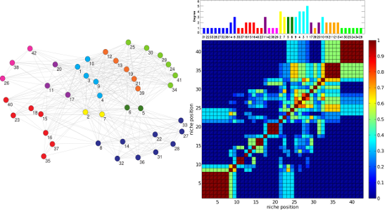
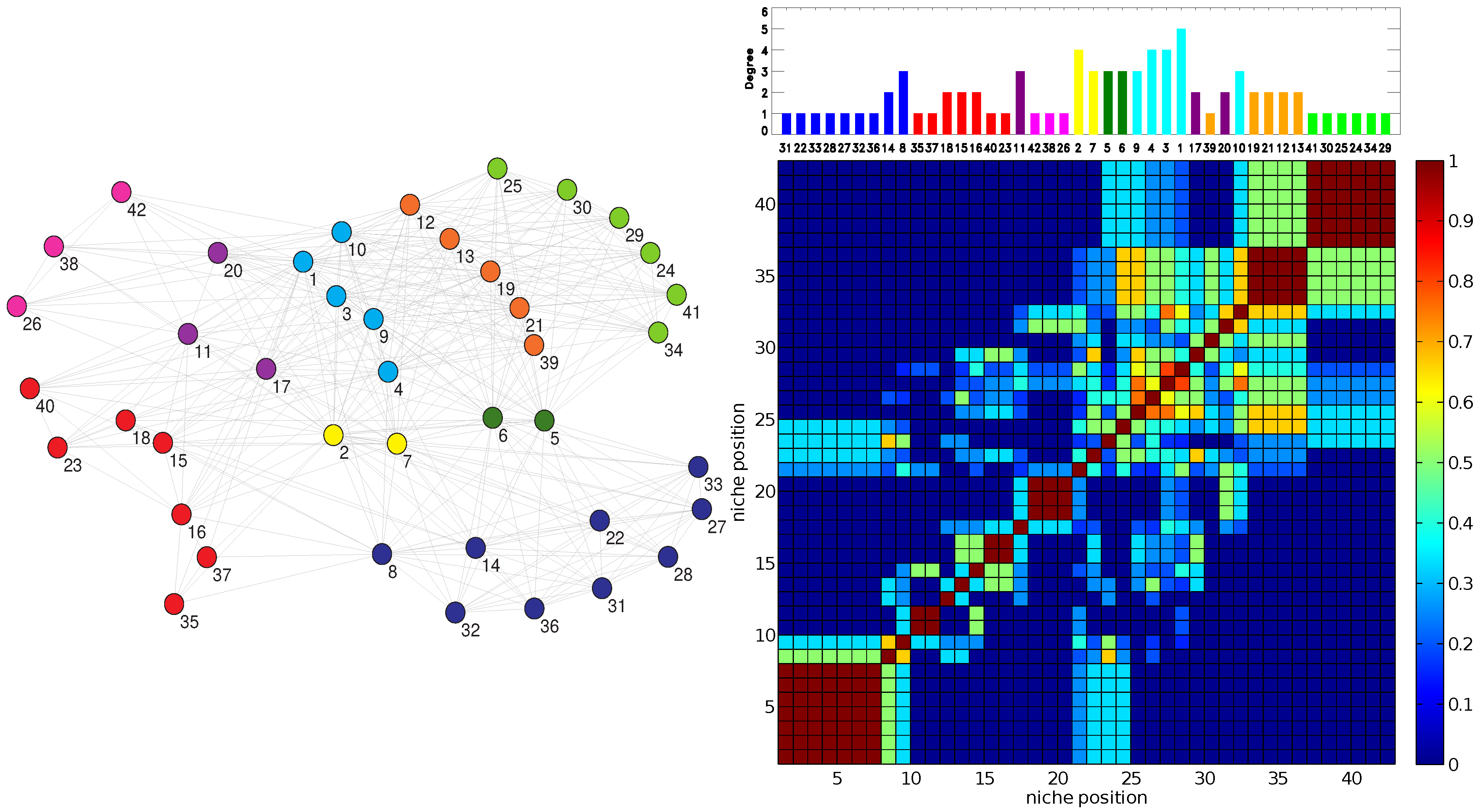
The RO method produces two clear patterns. Firstly, the Jaccard matrices display a block structure along the diagonal that corresponds to the niche axis (dark red blocks of a side greater than one in the right panel of
Figure 3). Such a structure is typical of Jaccard matrices computed by using MacArthur and Levins’ niche overlap [
20]. These blocks correspond to sectors of strong resource overlap. The blocks of maximum overlap,
= 1, occur for sets of specialists (
= 1 or 2) that all share one or at most two plants as their resource.
Secondly, the degree of generalism
versus the niche position,
, exhibits a pattern of “hills” separated by shallow “valleys” corresponding to alternating clusters of generalists and specialists (upper panel of
Figure 2 and
Figure 3). This undulated landscape can be understood, because as generalist species (plants or pollinators) have wider niches than specialists, the niche overlap between a generalist and a specialist is in general smaller than the niche overlap between pairs of generalists or pairs of specialists that share some resource.
In turn, these clusters of generalists or specialists are often associated with classes obtained when applying the EM method. Note in particular how in
Figure 3, the order and size of the contiguous EM classes in the right top panel closely follows the block structure along the diagonal of the resource overlaps depicted in the bottom right of the figure.
Figure 3.
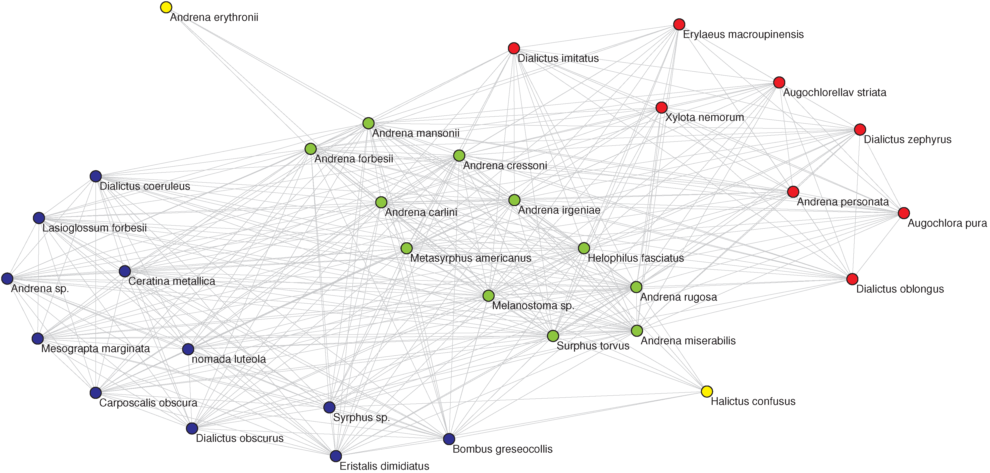
(Left) The OFST pollinator-pollinator network with the nine-fold EM classification. The color of each node denotes the class in which the pollinator has been classified by the EM algorithm. (Right, top) The corresponding plot of degree
D vs. inferred relative location on a one-dimensional niche axis (legend as in
Figure 2). The numbering of the pollinators corresponds to the IDs given in the data source [
27] and agrees with those in the left panel. (Right, bottom) The Jaccard
matrix measuring the resource overlap of species
i and
j.
(dark blue) corresponds to no resource overlap, while
(dark red) corresponds to complete resource overlap, in general only possible between two specialists with
that have the same resource.
Figure 3.
(Left) The OFST pollinator-pollinator network with the nine-fold EM classification. The color of each node denotes the class in which the pollinator has been classified by the EM algorithm. (Right, top) The corresponding plot of degree
D vs. inferred relative location on a one-dimensional niche axis (legend as in
Figure 2). The numbering of the pollinators corresponds to the IDs given in the data source [
27] and agrees with those in the left panel. (Right, bottom) The Jaccard
matrix measuring the resource overlap of species
i and
j.
(dark blue) corresponds to no resource overlap, while
(dark red) corresponds to complete resource overlap, in general only possible between two specialists with
that have the same resource.
Therefore, our analysis sheds light on how those groups of ecologically-similar species self-organize into niches based on the similarity of some of their biological traits and their abundance [
20]. Indeed, the niche concept is an important element in many aspects of ecological thinking, across levels of organization, from individuals (concerning their behavior, morphology and physiology) to ecosystems (to evaluate how species participate in ecosystem functioning) [
42]. The niche framework helps to devise each species place and role in the community to which it belong, as well as it provides a better understanding of species coexistence, new insights and interpretations about ecological patterns and processes in ecology and how fluctuating environments might regulate population dynamics and species interactions.
As we have seen, there are classes that emerge from a classification into a low number of classes
and persist while
increases. At the same time, there are classes that are refined as the number of classes increases. Both types of behavior can reveal meaningful information about the network. To illustrate these points, we consider the classifications of the DISH pollinator-pollinator network into
and 9 classes, as depicted in
Figure 4. Consider for example the set of pollinators with IDs
. These pollinators are classified as belonging to the same “green” group for all of the classifications shown. In fact, this turned out to be true for all classifications attempted
.
Figure 4.
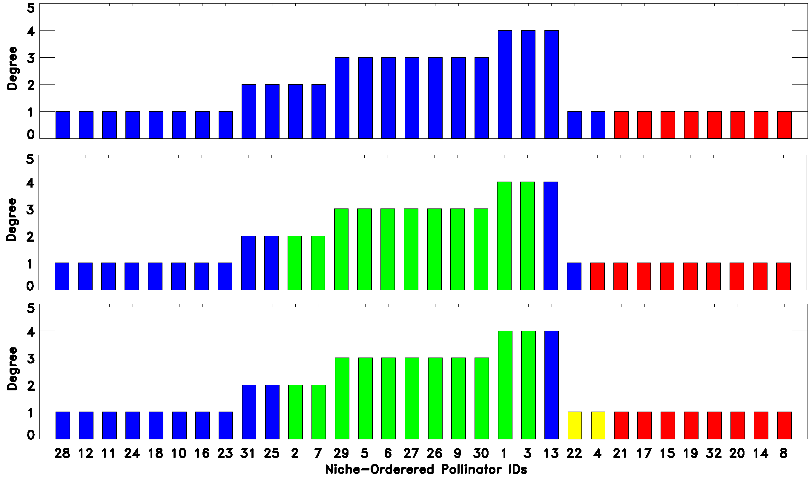
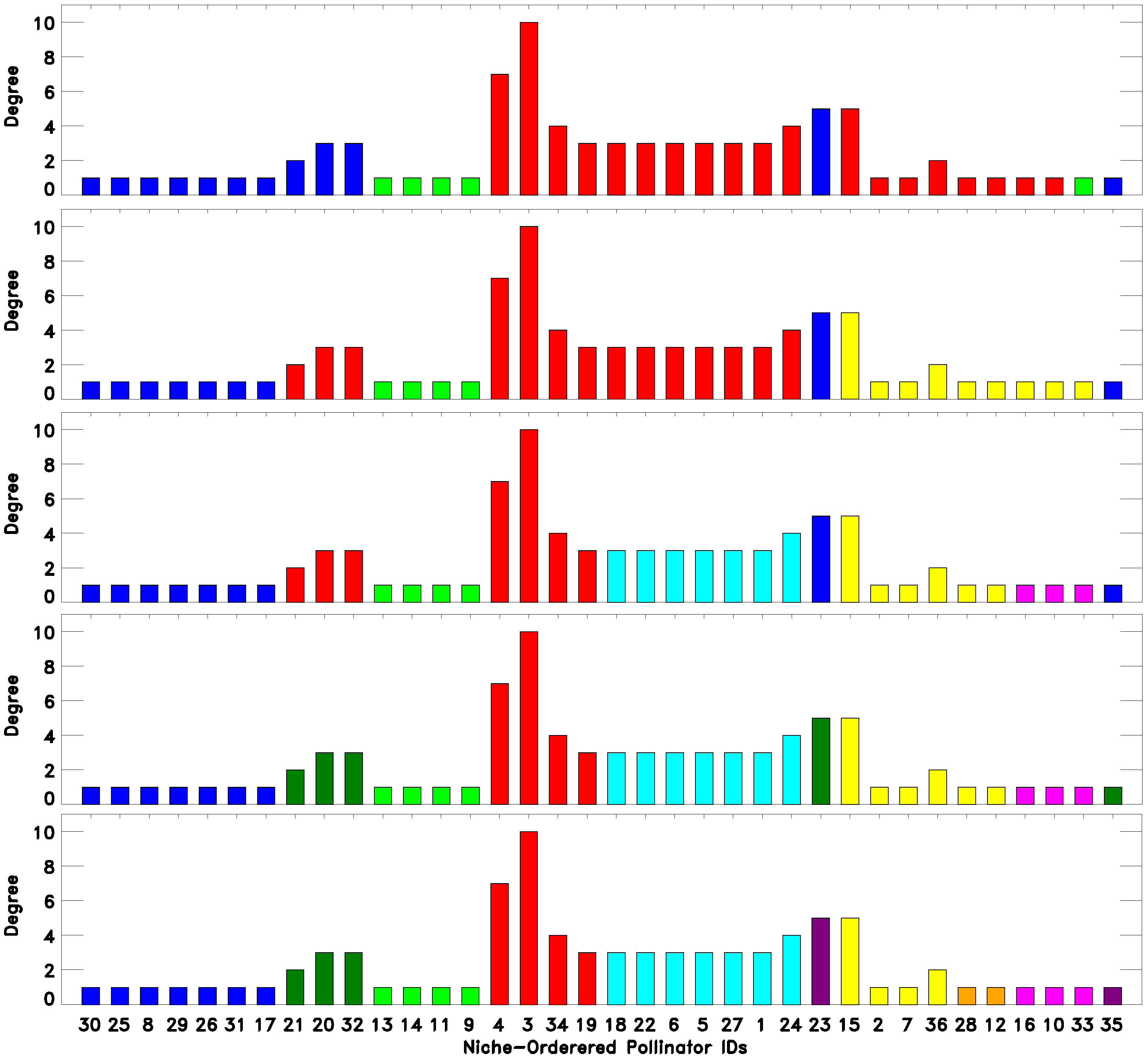
(Top to bottom) 3-, 4-, 6-, 7- and 9-fold EM classification of the DISH unipartite pollinator-pollinator network. As the number of classes increase, we see both robustness, namely certain species being classified together, as well as the emergence of finer structure, as classes are split up (legend as in
Figure 2).
Figure 4.
(Top to bottom) 3-, 4-, 6-, 7- and 9-fold EM classification of the DISH unipartite pollinator-pollinator network. As the number of classes increase, we see both robustness, namely certain species being classified together, as well as the emergence of finer structure, as classes are split up (legend as in
Figure 2).
On the other hand, most of the other classes, as expected, split up into smaller classes when
is increased. In this case, an increase of
often reveals the internal structure of a cluster of species. Again, for DISH,
Figure 4 considers the first ten species on the niche-axis,
. These 10 species constitute almost the whole blue class for the
classification, while when
, they split up into two classes, Species 21, 20 and 32 becoming part of the “red” class and then forming their own class when
. Likewise, comparing the three- and four-fold classifications, we see that the “red” class splits into two, forming a new class containing the pollinator IDs
, which coincides with the set of generalists (large degrees), at the center of the niche axis.
5. Conclusions
Ecological networks are an interdisciplinary research field, where physicists, biologists and applied mathematicians have been working together in order to understand the structure of ecological networks, one of the outstanding challenges in the study of complex systems.
The case of mutualistic interactions is of paramount importance; for example, we have seen that the mutualism between plants and pollinators is vital for the maintenance of most natural systems. Moreover, pollinators play a key role in communities, and their decline is leading to a crisis that is affecting both native and cultivated plant species [
43,
44,
45]. A better understanding of the structure of plant-pollinator communities and how this relate to their dynamics is key to developing models capable of explaining the relative species abundance. These quantitative models are useful for several purposes, like predicting the consequences of the loss of pollinators on crop yield [
46].
A recently-developed model for pollination, in terms of mutualistic interactions between plants and pollinators aggregated into classes with similar traits, was able to predict the relative abundances of plants and pollinators of a Mediterranean network [
30]. The problem is that only for a handful of these networks are there public data about species traits, like the nectar depth for plants and the proboscis length for animals, which seem to play a crucial role in determining the set of mutualistic interactions occurring between plants and pollinators [
36,
47,
48,
49,
50,
51]. The general procedure we proposed here, based on the combination of EM and RO, offers a possible alternative to overcome this lack of data on traits by classifying plants and pollinators into classes associated with clusters of species with overlapping niches (
i.e., grouped on a niche axis).
From quantitative interaction matrices,
, it is possible to compute using a generalization of Jaccard similarity indices, basically internal products, more refined overlap matrices and the corresponding species niche distributions [
20]. Something worth addressing in future work would be to extend the EM method in such a way as to incorporate quantitative information on mutualistic interactions. For example, we have formed the unipartite pollinator-pollinator networks by including a link between two pollinators when they have at least one common plant resource. However, it would be natural to consider weighted links, where the weight of a link is the quantitative amount of resource overlap for the two pollinators. Likewise, the number of visits of a pollinator to a plant could also be used as a quantitative input into the EM method.


