1. Introduction
The concept of entropy plays a key role in describing the transition between disorder and order. Specifically, the emergence of order in a random phase is indicated by a significant reduction of entropy. Calculating this reduction requires to know the probability of each possible system configuration that is compatible with the given system constraints—a challenging problem both methodologically and computationally. If we consider a system of N elements each of which can be in one of two states—for example up and down spins in a physical system, or agents with opposite opinions in a social system, or agents with the two strategies cooperate or defect in an economic system—the number of possible configurations is , which can be quite large. In fact, statistical physics was founded in the 19th century to provide an efficient solution based on the concept of statistical ensembles and state sums.
In this paper, we address the problem by proposing a stochastic approach that allows to decompose such probabilities for systems characterized by neighbor-neighbor interactions. Our candidate model to describe this interaction is the so-called
voter model which is discussed in more detail in
Section 3. In this model, agents are in one of two discrete states,
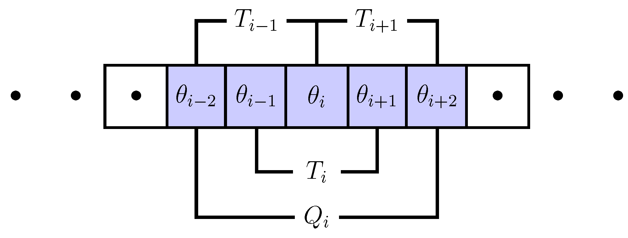
, denoted as “opinions”. They change their opinion in response to the opinions in their neighborhood. In order to define such a neighborhood, we have chosen a one-dimensional cellular automaton (CA), in which consecutively numbered cells
represent agents (see
Figure 1). We assume that the CA forms a ring to close the system. Each agent
i then has two neighbors
,
,
i.e., their opinions
form a triplet
. The second-order neighborhood that also takes the neighbors of
,
into account, then results in a quintuplet of opinions
.
Figure 1.
One-dimensional cellular automaton (CA) with triplet () and quintuplet () definition of the neighborhood of agent i.
Figure 1.
One-dimensional cellular automaton (CA) with triplet () and quintuplet () definition of the neighborhood of agent i.
Our major assumption of the voter model is that changes in the opinion of agent i are only caused by the first-order neighborhood. Specifically, the agent responds to the local frequency of opinions in the triplet that also includes its own opinion. However, because the dynamics of agent i depends on its neighbors, it is also coupled to their dynamics, i.e., to the second-order neighborhood of agent i, and so forth. This specifically denotes the problem that we are going to discuss in this paper. In a stochastic approach, we are faced with a system of N coupled dynamic equations for the probabilities to find any agent i with opinion at time t. This coupling exists only through the two neighbors of each agent, i.e., changes in a far distant cell only propagate slowly through the CA by means of neighbor-neighbor interactions. So, precisely, how large should be the neighborhood taken into account for the dynamics of the CA? Or, how far reaching are correlations in the changes of opinions?
To answer this question, in this paper we propose three different analytic approximations for the dynamics which take different neighborhood sizes into account: zero-order–no correlations between neighboring agents, first-order–correlations between an agent and one of its nearest neighbors (so called pair approximation), second-order–correlations between an agent and its second-nearest neighbors. We test the validity of these dynamic approximations by comparing them to stochastic simulations of the CA, averaged over a number of runs.
Our emphasis is of course on the second-order approximation, which extends previous investigations. But we want to understand under which circumstances this approximation fares better than the simpler ones. Therefore, we have chosen different variants of the voter model, also known as nonlinear voter models. The non-linearity is with respect to the response to the local frequency of opinions. We further compare deterministic and stochastic dynamics, to show whether our analytic approximations can correctly predict the dynamics. Our variable of interest is the expected fraction of opinion 1, denoted as , which is an aggregated variable for which we derive the dynamics based on a stochastic approach.
Our paper combines, and extends, previous investigations in different directions. One line of research refers to the approximation of higher-order probability distributions by means of lower-order distributions [
1] which has been also applied to the voter model [
2]. This implies a loss of (microscopic) information which can be quantified by means of information-theoretic measures [
3]. The question whether the coarse-grained dynamics is still Markovian can be answered by analyzing emergent macroscopic memory effects using information-theoretic measures [
4]. Such measures have also been applied to voter models [
5]. In most cases, the Markov chain analysis becomes quite cumbersome and therefore is restricted to one-dimensional CA [
6].
Another line of research considers different forms of neighborhood approximations specifically for binary state-dynamics (see [
7] for a good overview), which also has been applied to the voter model, already [
8]. We note that our pair approximation approach follows [
8], but applies it here to a one-dimensional CA, which results in different expressions for
and the correlations
.
Compared to two-dimensional CA [
9,
10] or even complex networks [
11,
12], one could find one-dimensional CA too simple. But this judgment is in fact not justified. Already one-dimensional CA have proven to exhibit a really complex dynamics, with a chance to derive analytic expressions. Extensions of the simple voter model, for example the Sznajd model [
13] or the
q-voter model [
14], could be thoroughly analyzed for one-dimensional CA.
The emphasis of our investigations is on the validity of the analytic approximations for nonlinear voter models. This non-linearity can be introduced in different ways. In References [
15,
16,
17], the authors discuss it on the level of individual agents that respond to neighboring influences in a heterogeneous manner. Specifically, Stark
et al. [
16] assumes a heterogeneous inertia for agents to change their opinions, Castellano
et al. [
15] assumes a heterogeneous neighborhood size to influence agents, while Xiong
et al. [
17] assumes a heterogeneous weight for the influence of agents.
Compared to these approaches, we assume a homogeneous, but nonlinear response of agents on the local frequency of opinions. Specifically, we consider the majority rule, where the tendency of agents’ to change their opinion increases with the frequency of the opposite opinion. The minority rule, on the other hand, assumes exactly the opposite, i.e., a decreasing tendency. This can be simply varied by one parameter α, which however is assumed to be the same for all agents.
Eventually, we would like to point out that we refrain from interpreting our model in a social context. Although agents are called “voters” and their states are called “opinions”, the simplicity of the underlying assumptions does not justify to sell the model as a reflection of a social system. We see it rather as a very generic setup to better understand the impact of local feedback on emerging systemic properties, such as consensus (
i.e., a “ferromagnetic” phase) or coexistence (
i.e., a “paramagnetic” phase). But we acknowledge that, despite this basic limitations, the voter model has been applied in various context, e.g., to model investors’ behavior in financial markets [
18], emerging communication networks [
19], or invasion of species [
20]. A good overview of spin-type models in sociophysics is given in [
21].
2. Stochastic Approach
2.1. Defining the Cellular Automaton
In this paper, we consider a one-dimensional CA consisting of
N cells, each of which is identified by the index
(see
Figure 1). Each cell shall be characterized by a discrete value
, hence the total distribution of states is given by the vector
. Assuming a torus space, each cell
i has a clearly defined neigborhood of first and second nearest neighbors,
and
. The probability to find cell
i in state
at time
t (where time shall be measured in discrete steps) is
. Consequently, the conditional probabilities
and
describe the probability to find cell
i in state
given that it has the first and second nearest neighbors
,
.
Under Markov assumptions the Chapman–Kolmogorov equation holds for the probability
to find cell
i in state
at time
:
The propagator
denotes the transition probability to go from any given state
at time
t to the assumed state
in the next time step,
. Here the summation is over all possible realizations
of
,
i.e., the
possible states
. At this point, we make our 1st assumption, namely that any change of
depends on the nearest neighbors, given by
. That means a triplet
decides about the value of
in the next time step. If we define the probability of a triplet configuration as
then the probability
results as the marginal distribution of the triplet probability:
Here the summation is over all possible realizations of the nearest neighborhood , i.e., different possibilities. denotes the conditional probability to find as the focal cell given a triplet , and the summation is over all possible realizations of , i.e., diffferent possibilities.
Based on the assumption that the nearest neighborhood matters, we can rewrite Equation (
1) as
where
denotes the conditional probability to find the focal cell in state
given the neighborhood
. Using Bayes’ rule, we can express this probability as:
With this, we can eventually rewrite the Chapman–Kolmogorov Equation (
1) for the single cell
i in terms of the triplet probabilities,
:
The propagator describes the transition probabilities to go from any possible triplet to a state during the next time step.
This equation leaves us with the further specification of the triplet probability,
. While, according to our 1st assumption, the occurence of
is just determined by the nearest neighbors
, the occurrence of either
or
also depends on their nearest neighbors,
i.e., the second nearest neighbors of
i,
. That means a quintuplet
decides about the value of the triplet
in the next time step. If we consider a quintuplet configuration
, then we can define the triplet probability as the marginal probability:
Here the summation is over all possible realizations of the nearest neighborhood , i.e., different possibilities. denotes the conditional probability to find the focal triplet given a quintuplet , and the summation is over all possible realizations of , i.e., diffferent possibilities.
For the dynamics for the probability to find a triplet in state
at time
, we can write a Chapman–Kolmogorov equation quite similar to Equation (
6)
The propagator describes the transition probabilities to go from any possible quintuplet to a triplet during the next time step.
In order to specify the quintuplet probability , we may consider a neighborhood of seven, etc. However, following the above procedure repeatedly is neither convenient nor practicable since at the end we have to consider possible configurations. Therefore, in the next section, we present a more convenient method to determine the quintuplet probability distribution.
2.2. Quintuplet Approximation
Instead of defining the quintuplet distribution in terms of higher-order probability distributions, following the procedure of the previous section, we now make our 2nd assumption by expressing these probabilities in terms of lower-order distributions, i.e., triplet distributions, this way arriving at a closed form description of the problem.
In the following we refer to the theory of approximating discrete probability distributions already developed in the late 1950 [
1], which was also applied to voter model (VM) [
2]. The idea is to approximate an
n-th order probability distribution,
by products containing the probabilities of given subsets, e.g.,
. It is known that such a product approximation contains at most
n terms, since every new term has to contain at least one variable
not contained in previous terms. For example, the factorization
already satisfies this condition, although it may be not a good approximation, since it holds only for ideal systems.
We note that the approximation procedure is not unique, i.e., there are various ways of constructing a product approximation. For example, taking , this can be approximated by as well as by or by . Which one of the above approximations is the most suitable has to be determined based on the information available about the triplet distribution . In some cases, there are measurements of this distribution, or additional information about the dependency between the as we will use below.
With reference to our quintuplet approximation using the triplets defined, we propose the following procedure: we first note that there are different triplets contained in the quintuplet configuration, for example:
,
,
. These are valid triplets because they consider the correct neighborhood relations, whereas for example
would be inappropriate. Out of the valid triplets, we may choose for example the first one,
and complete the product approximation as follows:
In order to express the conditional probabilities using the triplet distribution, we apply Bayes’ rule:
which results in the final quintuplet approximation:
We note that this product approximation is the only possible one, given that we have an ordered set of variables according to their neighborhood relations.
2.3. Closed Form Dynamics
Using the approximation explained above, we have reduced the higher-order description to the level of triplet distributions,
,
etc., which results in a closed form dynamics. We now have to specify the initial conditions for the distributions. While we are able to make any suitable assumption about the initial triplet distribution, we assume here that the occupation of the different cells is initially statistically independent,
i.e.,
For further investigations, we have set .
In order to solve the above set of equations, we have two different possibilities: we can solve the dynamics (a) on the level of the distribution
, Equation (
6), or (b) on the level of the triplet distribution
, Equation (
9). Variant (a) requires more computational effort, since we have to replace any
as a marginal distribution of triplets, whereas in variant (b), given the reduction of the quintuplet distributions, we already have a closed form dynamics for the triplet distributions, which is computationally more efficient.
Variant (b), however, requires to know the transition probabilities on the level of the triplets, whereas these are usually specified on the level of single cell changes (see also the following section). Hence, we have to determine the propagators
in terms of
. Since our 1st assumption specifies that the change of every cell in the triplet only depends on its nearest neighbors, we are able to factorize these transition probabilities:
This completes our closed form description. To calculate the time-dependent probability distribution of triplets, we have to insert Equation (
12), Equation (
14) into Equation (
9) and from the result calculate
as the marginal distribution, Equation (
3). The only remaining task is now to specify the transition probabilities for single cells,
at which point the VM comes into play.
3. Nonlinear Voter Dynamics
3.1. Transition Rates
The voter model, in its basic form, is applied to a population of N agents, where each agent is characterized by a discrete value, its “opinion”, . The opinion dynamics at the level of the agents works as follows: two agents i and j are randomly chosen from the population, and agent j adopts the opinion of agent i, i.e., . After N such update events, time is increased by 1 (random sequential update).
The rather simplified rule limits the applications of the voter model to any real voting process or opinion dynamics. In a well mixed population, the probability for agent
j to adopt a given opinion
is simply proportional to the global frequency
of agents with the respective opinion:
This dynamics is known to always converge to complete consensus, or . The only interesting question is then how long it will take to reach this state dependent on the system size N and the initial condition .
This picture becomes more complex if instead of a well-mixed population a defined neighborhood for each agent is assumed. This can be a social network where agents have links to other agents, or simply a lattice where the neighborhood is given by the geometry that defines the nearest and second nearest neighbors of an agent. Then, instead of the global frequency, the probability of an agent to adopt a given opinion depends on the local frequency,
, of this opinion in the neighborhood of that agent:
Here means the Kronecker delta, which is 1 only for and zero otherwise. In this paper, we restrict ourselves to the one-dimensional regular lattice, where each agent is represented by a cell i that has precisely two neighbors. Different from the basic voter rule, in the calculation of the local frequency we have taken the opinion of the focal cell i into account. This adds some inertia to the dynamics as agent i counts towards the local minority/majority. It also avoids stalemate situations where the two neighbors have different opinions.
The linear voter model would assume that the transition rate
of a focal cell
i to change its opinion from
to
is directly proportional to the local frequency
,
i.e., the opposite opinion in the neighborhood. The expression of Equation (
17) is a specification of the more general transition probability
used in Equation (
14). It takes into account that for frequency dependent processes the change of
depends not directly on the local distribution
, but only on the local frequency
.
We are more interested in the non-linear case, where the local frequency still plays a role, however the response to the opposite opinion can be different. The linear voter model can then be generalized into a majority rule where the transition toward the opposite opinion monotonously increases with the respective local frequency. Different from this, the minority rule would assume that the transition toward the opposite opinion monotonously decreases with the respective local frequency, i.e., the minority opinion is favored. Eventually, we could also have mixed rules with a non-monotonous frequency dependence, which become possible only if the local frequency depends at least on the opinion of three agents, as it is the case in our model.
Instead of an analytical expression, we specify the transition rate
by using free parameters
,
,
,
which cover all of the above cases in a general manner. With these, the transition rates shall be defined as follows:
The general case of four independent transition rates in Equation (
18) can be reduced to two transition rates
,
by assuming a symmetry between the two states 0 and 1,
i.e.,
,
. The condition
then denotes the above mentioned majority rule, because the transition rate increases with an increasing fraction of the opposite opinion
in the neighborhood. This process is also known as positive freqency dependent invasion. In ecology, it means that individuals of abundant species have a better chance to survive.
Opposite to that, for the so-called negative freqency dependent invasion process the probability that cell
i shall switch to the opposite opinion
decreases with the fraction number of individuals of subpopulation
σ in the neighborhood. This implies
In an ecological context negative frequency dependent invasion means that individuals of a rare subpopulation have a better chance to survive.
The rate
in Equation (
18) applies for the case where cell
i is only surrounded by opinions of the same kind. In a deterministic model, there would be no force to change the current state. In a stochastic CA however all possible processes should have a certain non-zero probability to occur, therefore a rather small value
is used to avoid absorbing states in the dynamics. We will then only vary the remaining rate
, which is the only free parameter in the model. Table summarizes the different transition rates given the possible local configurations
. It should be read as follows: given that the local configuration is e.g.,
at time
t, the probability to find
is
α. If
this transition rate increases with
, hence it denotes a majority voting rule, otherwise it denotes a minority voting rule.
Now that the transition rates for the nonlinear voter model are specified, we have different ways to proceed: (1) We can run stochastic computer simulations of the one-dimensional CA, to get some intuition about the dynamics and the role of the parameter
α. This will be described in the following
Section 3.2; (2) We can also derive an approximate macroscopic dynamics for the global frequency
, which will be done in
Section 3.3 and
Section 3.4 using two different approximations; (3) Eventually, we can use the closed-form description already derived in
Section 2.3, to numerically calculate
. The stochastic simulations will denote our reference case, used to compare the two different approximate macroscopic dynamics and the numerical calculations.
3.2. Computer Simulations of the CA Model
For a first insight into the dynamics, we have conducted stochastic simulations of the CA described above. In this section, we will only refer to particular runs, to show some snapshots of the dynamics, while in
Section 4 also averaged simulation results of the global variables are discussed.
For our simulations, we have used a one-dimensional CA of
cells with periodic boundary conditions, where all cells are simultaneously updated. The discrete time scale is defined by generations. We have checked that the main results do not change if
N is increased to 6400. The initial configuration of the CA refers to a homogeneous distribution (within discrete limits) of both opinions,
i.e., initially each cell is randomly assigned one of the possible states,
, with a probability that is equal to the initial global frequency
. At each time step, the transition rates are calculated for each cell according to Equation (
18) and the values are compared with a random number
rnd drawn from the intervall
. If
rnd is less than the calculated transition rate, the respective transition process is carried out, otherwise the cell remains in its current state. Since each transition only depends on the current local configuration, memory effects are not considered here.
It follows from the above description that the case and refers to a deterministic positive majority voting rule, simply because the state of cell i never changes unless the two nearest neighbor cells have adopted the same opinion. However, then, it will always change, such that all three cells have the same opinion. Similarly, a deterministic minority voting rule is described by , and .
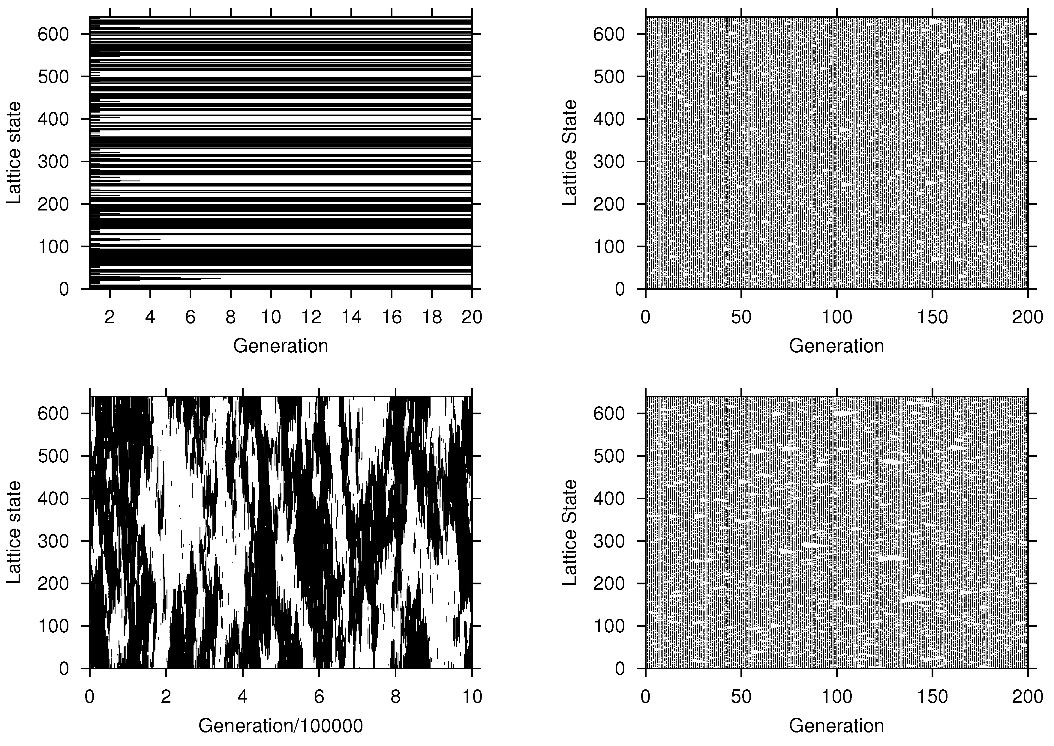
The results of the computer simulations are illustrated in
Figure 2. We first note the remarkable difference in the outcome between majority and minority voting. In the latter, cells change their state frequently, however no pattern evolves because the cell always adopts an opinion different from the two neighbors, if these have the same opinion. Thus, we see a rather random and unstructured pattern, in which both opinions coexist with a long-term fraction
. This overall behavior is also not changed in case of a stochastic dynamics.
Figure 2.
Evolution of the cellular automaton (CA) for different rules: (left column) majority voting; (right column) minority voting; (top row) deterministic dynamics; (bottom row) stochastic dynamics. Parameters: (top left) , , (top right) , , (bottom left) , , (bottom right) , . , initial condition: , (black) indicates , (white) indicates .
In contrast, for the majority voting rule we observe the formation of local clusters of the same opinion. In the deterministic case, the resulting pattern becomes stationary very fast, such that the clusters remain rather small. In the stochastic case, however, we observe the interesting phenomenon that very large clusters of cells with the same opinion emerge. These domains do not grow up to system size because of the small perturbation
, that enables cells to adopt a different opinion even in a homogeneous neighborhood. The non-linearity (
is different from the linear case
) then amplifies such random deviations. This phenomenon has been discussed, for the case of a two-dimensional CA, in [
8]. As a consequence, we observe a correlated coexistence of both opinions characterized by the facts that (i) each opinion at times is the majority and (ii) forms larger clusters, and (iii) the dynamics is always in non-equilibrium. This is clearly visible in the long-term behavior, shown in
Figure 2 (bottom left).
In
Section 4, we further investigate these different regimes numerically, after we have derived some appropriate approximations of the macroscopic dynamics.
3.3. Derivation of the Macroscopic Dynamics
A formal description for the dynamics of the CA starts with the probability
used in Equation (
1). By means of
we can obtain the key variable of the macroscopic dynamics
, which is the expected global frequency of each opinion in the population. Note that, different from Equation (
15) where
is used,
describes the ensemble average over very many simulations. This is of some importance when interpreting the results. For the linear voter model, it is known that the system converges always to consensus,
i.e.,
or
. If we use the initial condition
, then in 50% of the cases we observe
, and in 50%
. However, when averaging over all of these outcomes, we find
.
Assuming a master equation for the dynamics of
with the transition rates specified in Equation (
18), we can derive a rate equation for
as discussed in detail in [
8]:
Here, the summation is over all possible
opinion patterns
for the neighborhood of cell
i. These are binary strings
that indicate the particular values of the nearest neighbors
,
. With
neighbors, these would be 00, 01, 10, 11. Together with the possible state for cell
i,
i.e.,
or
, the respective local frequencies
can be derived according to Equation (
16), such that all transition rates in Equation (
22) are specified. The solution of Equation (
22) would however require the computation of the averaged global frequencies
and
for all possible opinion patterns
over time, which would be a tremendous effort. Therefore, in [
8] two analytic approximations have been discussed to solve this problem. Here, we only summarize the results.
In the first approximation, the so-called mean-field limit, the state of each cell does not depend on the opinion of its neighbors, but is only influenced via a mean field. In this case the opinion distribution factorizes:
and we find with
for the macroscopic dynamics, Equation (
22) in the mean-field limit:
For the calculation of the
we have to look at each possible opinion pattern
. The mean-field approach assumes that the occurence of each 1 or 0 in the pattern can be described by the global frequencies
x and
, respectively (for simplicity, the abbreviation
will be used in the following). Taking the example 100,
i.e.,
for cell
i and
,
for its neighbors, would result in
. Inserting further the transition rates, Equation (
18), we find this way the equation for the mean-field dynamics as:
The fixed points of the mean-field dynamics can be calculated from Equation (
25) by means of
. In the limit
, we find:
The three stationary solutions denote either consensus toward one of the opinions, or coexistence of both opinions with an equal share. In order to verify the stability of the solutions, we have further investigated the Jacobian
of Equation (
25). The results can be concluded as follows: Below a critical reinforcement,
,
and
are stable attractors and
is the separatrix. Above the critical reinforcement,
,
becomes the stable attractor, while
and
are unstable. We will come back on this after discussing the second approximation.
3.4. Pair Approximation
The mean-field approximation assumes that the local occurrence of opinions is determined by the global frequencies rather than by local interactions. A better approximation should take local correlations between neighboring cells into account. Our second approximation, the so-called pair approximation, is based on the assumption that the state of each cell i is only correlated to the states of each of its nearest neighbors, separately. i.e., the two neighbors are only correlated through the focal cell and not to each other. Therefore, the neighborhood is decomposed in pairs of nearest neigbor cells, , which are called doublets. The expected value of the global frequency of doublets is denoted as where σ refers to the focal cell and to one of its neighbors.
We can then approximate the global frequency of a specific opinion pattern
in Equation (
22) as:
where the
are the correlations:
that depend on the doublet frequency
and the global frequency of opinions
neglecting higher order correlations.
can be interpreted as the conditional probability that a randomly chosen nearest neighbor of a cell in state
is in state
σ. With the relations:
and using again
, these correlations can be expressed in terms of only
and
as follows:
We then find for the macroscopic dynamics, Equation (
22), in pair approximation:
With respect to Equation (
30), Equation (
31) now depends on two variables,
and
. In order to derive a closed description, we need an additional equation for
, that can be obtained from Equation (
28):
Equation (
32) requires additionally the time derivative of the global doublet frequency
. We note that the three coupled equations for
,
and
can be easily solved numerically. In the
Appendix, we have derived explicit expressions for these equations for the one-dimensional CA discussed here, using the transition rates of Equation (
18).
5. Conclusions
With our investigations of the one-dimensional voter model, we want to achieve two goals: (i) a better understanding of the non-linearity in the voter dynamics that was mostly studied as a linear model, only; (ii) a probabilistic description, and possible approximations, of the dynamics for the fraction of opinion 1, .
The non-linearity can be easily expressed by means of a free parameter α. The critical value distinguishes between two different rules, majority voting () and minority voting (), whereas refers to the border case of the linear voter model. It is known from well-mixed populations that majority voting should result in consensus, i.e., the asymptotic dominance of only one opinion, whereas minority voting should result in coexistence, i.e., the occurrence of both opinions in different fractions.
Our main focus was the role of local correlations in determining this outcome. For this we have used one-dimensional cellular automata (CA) in which each cell
i, characterized by its opinion
, has a defined neighborhood of two cells with possibly different opinions, denoted as triplet. The transition probability of a cell to change its opinion is then determined by the local frequency of opinions in its neighborhood (including the focal cell) and the non-linear response to this information, expressed by means of
α. The values of
α define a certain probability to switch to the opposite opinion,
i.e., we can use them to switch between a deterministic (
) or a stochastic (
) dynamics. In the latter case, we have further assumed a very small probability
to perturb a state of complete consensus, which allows a non-stationary dynamics of the CA as shown in
Figure 2 (bottom right).
While the minority rule only results in random coexistence of the two different opinions, the majority rule generates more interesting results. In particular, we observe a correlated coexistence characterized by the formation of large domains of the same opinion which change continuously. i.e., we have a non-equilibrium dynamics in which each opinion, for a certain time, can form large clusters of the majority opinion.
The question then is how to describe this dynamics mathematically. In this paper, we follow a probabilistic approach, i.e., each cell has a certain probability of a given opinion , which also depends on the probabilities of the nearest neighbors, second-nearest neighbors, and so forth. In order to close the dynamics, we have proposed three different approximations at different levels of the description.
The first level is the aggregated description in terms of the global fraction of opinion 1, , for which we derive a dynamics for the expected value, . On this level, we discuss two approximations. The simplest one is the mean-field approximation, in which no correlations between neighboring states are considered. So, we call this the zero-order approximation. It gives us a prediction for derived from the well-mixed case. In contrast, the pair approximation considers a correlation between a cell and its neighbor, i.e., the triplet consisting of a cell and its two neighbors is decomposed in two cell-neighbor pairs. Correlations between neighbors are not considered, so we call this the 1st-order approximation. Hence, we have a prediction for coupled to the dynamics of the pair correlations .
The third approximation does not refer to the aggregated level, but to the stochastic dynamics of a triplet, i.e., a cell with its two neighbors, that is determined by the larger neighborhood of a quintuplet, i.e., considers also the second nearest neighbors of the cell. Therefore, we call this the 2nd-order approximation. Using certain assumptions, we are able to provide a closed form dynamics for this larger neighborhood in terms of a probabilistic equation.
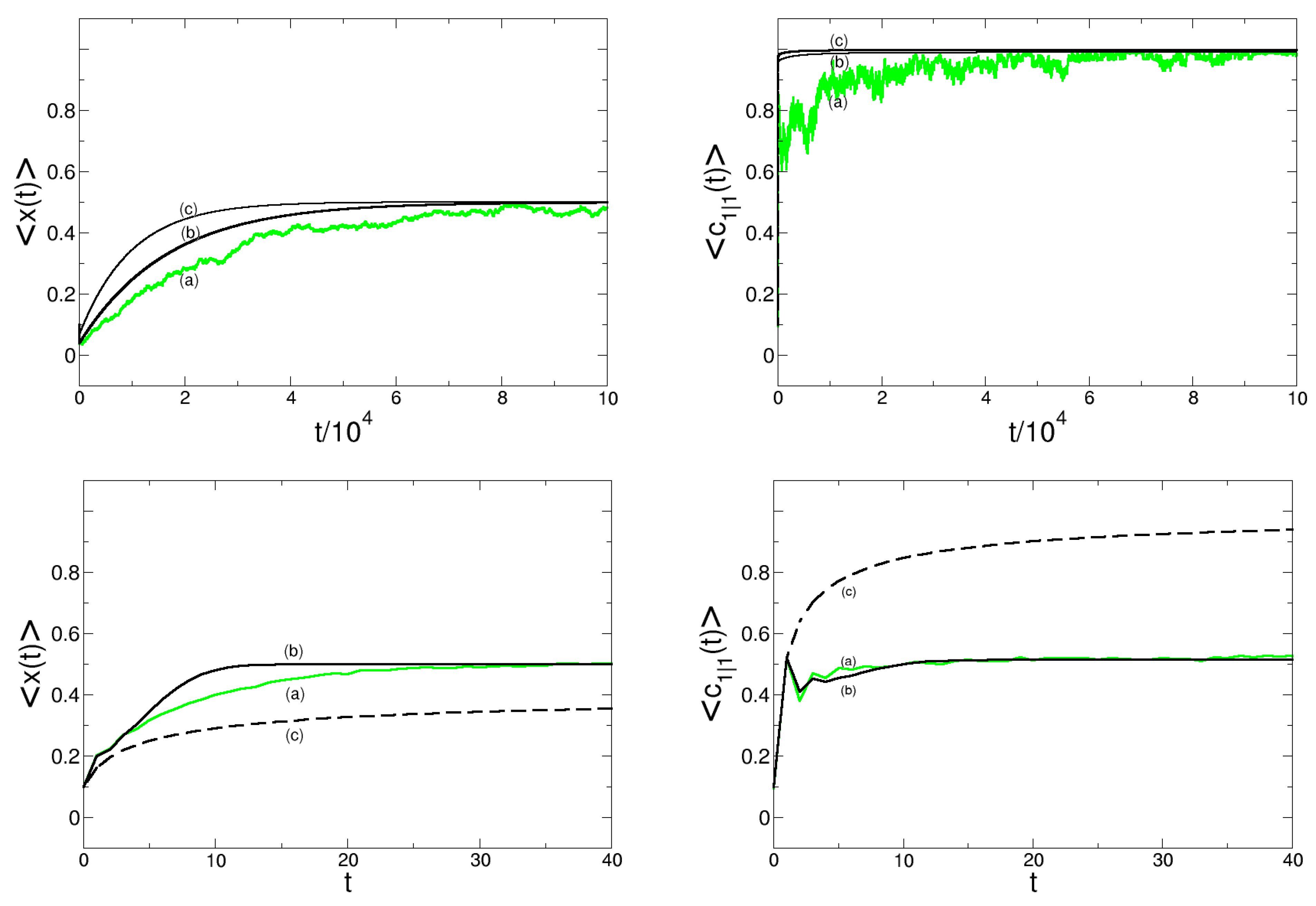
To compare the validity of these mathematical approximations, we use as a reference case stochastic computer simulations of the one-dimensional CA, which are averaged over a larger number of runs. We have discussed the majority and the minority voting, as well as the deterministic and the stochastic dynamics, separately.
In conclusion, we can summarize that the zero-order approximation only predicts the stationary outcome of the minority voting correctly, but fails for the majority voting rule, both with respect to the dynamics and the stationary outcome.
The first-order approximation performs comparably well in comparison to the second-order approximation only for the majority voting. The stationary outcome is correctly predicted both for the deterministic and the stochastic case, also the dynamics is covered fairly good. However, the first-order approximation fails to predict the dynamics of the minority voting. This case is only well covered by the second-order approximation that gives not only a correct description of , but also of the pair correlations .
Commenting specifically on the correlations, we recall again that both the first and second-order approximations lead to comparably good asymptotic results only for the majority voting. But they clearly predict a faster formation of domains, i.e., a convergence to their stationary value, as compared to the CA simulations. This limits their usability to fully understand the emergence of long-range correlations. In the case of minority voting, our first-order approximation fails, while the second-order approximation for could be even seen as accurate in its computational prediction. This is not so surprising if we recall that minority voting rules, different from majority voting, do not result in long-range correlations.
Hence, we can conclude that the quintuplet approximation that covers also the second-order neighborhood, is accurate enough to describe the dynamics of the CA on the macroscopic level. While it is of course understandable, that an approximation that considers more information is usually more accurate, we should also relate this conclusion to the computational effort. Here, it turns out that the 2nd-order approximation, although stochastic,
i.e., needs to be averaged over a number of runs, performs very fast because of the closed form dynamics. Of course, the 1st-order approximation, the closed form of which is given in the
Appendix, is computationally even simpler. But there is a trade-off with the accuracy of the prediction. Still, as long only majority voting is considered, the 1st-order approximation should be preferred, both for simplicity, accuracy and computational effort.
Our last remark is about the coexistence of the two opinions, which is the more interesting scenario compared to consensus,
i.e., the existence of only one opinion. Here, we are not so much interested in the trivial case of random coexistence without any structure formation, which is characterized by
and
. We focus more on the case of correlated coexistence which has an interesting complexity because of the formation of local structures, nicely shown in
Figure 2 (lower left). On the level of our approximations, this state is characterized by
and
.
i.e., both opinions form at times large domains, indicated by the high pair correlation, but none of the two opinions entirely dominates the dynamics, as the expected value for its fraction is about 0.5.
Such insights can be generalized to other cases of frequency dependent processes which e.g., play a role in population ecology (invasion or extinction of species). For most of these applications a two-dimensional CA is more appropriate as it was discussed in [
8]. The one-dimensional CA investigated here, on the other hand, allows a mathematical approximation of the stochastic dynamics in terms of the 2nd-order neighborhood, which gives a much higher predictive power. This formalism can be also used for other frequency dependent processes in one-dimensional CA.


