Distributed Control of Heat Conduction in Thermal Inductive Materials with 2D Geometrical Isomorphism

Abstract

In a previous study we provided analytical and experimental evidence that some materials are able to store entropy-flow, of which the heat-conduction behaves as standing waves in a bounded region small enough in practice. In this paper we continue to develop distributed control of heat conduction in these thermal-inductive materials. The control objective is to achieve subtle temperature distribution in space and simultaneously to suppress its transient overshoots in time. This technology concerns safe and accurate heating/cooling treatments in medical operations, polymer processing, and other prevailing modern day practices. Serving for distributed feedback, spatiotemporal H_∞/μ control is developed by expansion of the conventional 1D- H_∞/μ control to a 2D version. Therein 2D geometrical isomorphism is constructed with the Laplace-Galerkin transform, which extends the small-gain theorem into the mode-frequency domain, wherein 2D transfer-function controllers are synthesized with graphical methods. Finally, 2D digital-signal processing is programmed to implement 2D transfer-function controllers, possibly of spatial fraction-orders, into DSP-engine embedded microcontrollers.

1. Introduction

In the works [1,2] and the references cited therein, we learned that many materials possess measurable entropy-flow storage, and that heat conduction in these thermally inductive materials behaves as a standing wave whenever the heat conduction region is small enough to some extent of engineering practice. Known from modal decomposition of standing waves, modes of larger (smaller) variations in space have faster (slower) motions in time. Therefore, tracking of spatially subtle distributions of temperature under feedback control with pointed actuation will always be accompanied by temporally abrupt transients, resulting in unsafe or inaccurate heating/cooling treatments in medical operations, polymer processes, and other prevailing modern day practices.

To remedy such a situation, this paper continues to develop distributed control for non-Fourier heat conduction, inasmuch as distributed sensors and actuators are well-developed nowadays [3–14]. Distributed control is capable of tracking precise local-temperatures with slow heating over the entire region of heat conduction, which is otherwise beyond the nature of pointed control.

The systems & control literature documents several kinds of feedback technologies applicable to distributed control of non-Fourier heat conduction, which are collected in

Table 1. Candidate types of control for non-Fourier heat conduction.

Methodology	Typical references	Critical comments
1D control technology	Bamieh et al. [15] Stewart et al. [17] Gorinevsky et al. [19]	Finite-dimensional controllers based on order-truncated plants; thus, it is hard to track robust performance imposed on the originally distributed parameter plants.
Infinite transfer function	Callier and Desoer [20] Callier and Winkin [21] Callier et al. [22] Grabowski and Callier [23]	Having been theoretically well-developed for classical control systems with pointed sensing and pointed actuation.
Fraction-order dynamics	Podlubny [24] Valerio and Costa [25] Vinagre and Feliu [26] Monje et al. [27] Padula and Visioli [28]	An attractively empirical tool for feedback loopshaping with pointed sensing and actuation; usually being used in conjunction with frequency-domain identification. Requiring further developments on internal stability issues.
nD state space	Valcher [29–30] Fornasini and Valcher [31] Shu et al. [34] Lancaster and Zaballa [32] Carlos and Anaya [33]	Extension of 1D robust state-space synthesis upon nD discrete plant for nD discrete controller. Belonging to distributed control technique usually resulting in either overabundance or shortage of controller orders.
Distributed H∞/μ loopshaping	Hong [42]	Being 2D-version loopshaping upon continuous nD plant for 2D transfer function controllers. Graphically finding all feasible controllers with robust performance. Facilitating the identification of generalized plant in mode-frequency domain.

. Listed in the first entry are finite-dimensional feedback syntheses based on order-truncated plants, for examples [15–19], which in essence belong to 1D control methodology. For non-Fourier heat conduction, we consider them inadequate to track the robust performance specified both in space and in time. The second and third entries concern infinite dimensionality, wherein Grabowski, Desoer, Callier, Winkin [20–23], and others have adequately developed spectral factorization, algebra of transfer functions and semigroup theories applicable to control purposes. In practice, an infinite-dimensional transfer function from pointed input to pointed output can further be identified in the frequency domain with fraction order [24–28], serving for 1D-H_∞/μ feedback loopshaping. Unfortunately, these dimension-infinitely elegant tools were not originally developed for distributed sensing and actuation.

The fourth entry is suitable for a distributed control strategy, where the nD state-space robust control [29–34] is extended from 1D robust state-space synthesis to an nD version in the space-time domain. Controllers from state-space syntheses have spatiotemporal orders close to that of the generalized plant, usually resulting in either order-overabundance or order-shortage in that feasible controllers merely exist in much lower orders or in higher orders, respectively. Since microcontrollers that implement feedback control have limited computation and memory capability, high-order controllers will retard on-line processing of dynamics. Partly for this reason, we develop distributed H_∞/μ loopshaping to synthesize 2D transfer-function controllers of proper orders, listed in the last entry of Table 1. In this method, the generalized plant composed of the nominal plant, performance weightings and modelling uncertainty bounds is identified or specified in a mode-frequency domain, served for 2D-μ loopshaping in the mode-frequency domain for robust performance both in time and in space. It is extended from the conventional H_∞/μ loopshaping [35] in the frequency domain to 2D version in mode-frequency domain, named 2D- H_∞/μ loopshaping.

The so-called 2D transfer-function above is a functional representation of spatiotemporal dynamics through 2D integral transforms, with two independent variables representing the space and time, respectively. The systems & control literature documents several kinds of 2D integral transform, as listed in

Table 2. 2D transfer function modelling.

Methodology	Typical documents	Critical comments
Double Laplace transform	Dahiya and Vinayagamoorthy [36] Eltayeb and Kilicman [37]	Suiting for semi-infinite space regions with initial conditions in space and time.
Double Fourier transform	Bamieh et al. [15] Stewart et al. [18] Gorinevsky et al. [19]	Being applicable to signal processing and feedback loopshaping in two-side infinite space regions.
Laplace-Galerkin transform	Rabenstein and Trautmann [38–39] Hong [42] Hong et al. [2]	On bounded space regions has it been well justified to work.
Fourier-Galerkin transform	Hong [42]	A 2D geometrical isomorphism for distributed loopshaping on bounded regions

. Therein, the Double Laplace transform, for example in [36,37], and Double Fourier transform, for example in [15,17,19], were always applied for signal processing and feedback control in semi-infinite and infinite space regions, respectively. The Laplace-Galerkin transform [1,38–40] or Fourier-Galerkin transform [41,42] is justified to model the non-Fourier heat conduction and its controllers for bounded space regions that are of real concern in heat conduction practice. Such an integral transform is obtained through the composite of Laplace transform in time and modal decomposition in space. With the Laplace-Galerkin transform, Hong [42] developed the 2D-geometric isomorphism for 2D-μ loopshaping in mode-frequency domain. Later on, Hong et al. [2] applied 2D transfer-function modelling to prove that the time-delayed heat condition is an ill-posed description that contradicts the first law of thermodynamics. For convenient computation in 2D or 3D space regions, the 2D transfer functions can be numerically treated as 3D or 4D transfer-functions, respectively.

2. 2D Transfer-Function Modelling

Consider the non-Fourier heat conduction in a bounded region Ω. It is governed by energy conservation:

$$\rho C_v\frac{\partial T}{\partial t}+\nabla ·\mathit{q}=Q,$$

(1)

and the non-Fourier law:

$$R\mathit{q}+L\frac{\partial \mathit{q}}{\partial t}=-\nabla T,$$

(2)

where the thermal inductance L is included to fulfill the electro-thermal analogy [1]. Apart from thermal inductance L, a differential volume of Ω is of thermal resistance R and thermal capacitance C = ρC_v, where ρ stands for mass density and C_v for specific heat at constant volume.

Substituting Equation (2) into Equation (1) yields a hyperbolic equation:

$$\tau \frac{{\partial }^{2}T}{\partial t^2}+\frac{\partial T}{\partial t}-\frac{1}{C}\nabla ·\left(k\nabla T\right)=\frac{1}{C}\left(\tau \frac{\partial Q}{\partial t}+Q\right).$$

(3)

wherein k stands for the thermal conductance, k ≡ 1/ R, and τ for the relaxation time in heat diffusion τ ≡ L/ R, with the following assumptions in practice:

(A1)

the first-order spatial derivative of the thermal conductance k exists, and

(A2)

the nominal value of relaxation time in heat diffusion τ is uniformly distributed over the operation region Ω.

Let the temperature distribution and heat-rate source be scaled by a reference temperature T̄ as ψ ≡ T / T̄ and q ≡ Q /CT̄, and then we can rephrase the hyperbolic heat-conduction to be:

$$\tau \frac{{\partial }^2\psi }{\partial t^2}+\frac{\partial \psi }{\partial t}-\frac{1}{C}\nabla ·\left(k\nabla T\right)=\tau \frac{\partial q}{\partial t}+q,\text{in\hspace{0.17em}}\mathrm{\Omega }\times {\mathfrak{R}}^{+}$$

(4)

where q represents the dimensionless entropy-rate flowing into the control region. The following boundary conditions are considered:

$$\alpha \psi +\beta \nabla \psi ·\widehat{n}=0\mathrm{\hspace{0.17em} }\text{on\hspace{0.28em}}\partial \mathrm{\Omega },$$

(5)

with α (x) · β (x) ≥ 0 for all x ∈ ∂Ω, which includes von-Neumann, Dirichlet, and Robin homogeneous boundary conditions.

The dynamics governed by Equations (3) and (4) involves the non-uniform operator defined over the set of spatial functions φ ’s ∈ L₂ (Ω):

$$\begin{array}{c}\mathcal{a}\phi =-(1/C)\nabla ·(k\nabla \phi )\mathrm{\hspace{0.17em} }\text{in\hspace{0.28em}}\mathrm{\Omega },\\ \alpha \phi +\beta \nabla \phi ·\widehat{n}=0\mathrm{\hspace{0.17em} }\text{on\hspace{0.28em}}\partial \mathrm{\Omega }.\end{array}$$

(6)

Based on the Sturm-Liouville theory [43], the eigenvalues of the non-uniform operator are all positive, and its eigenfunctions can constitute an orthonormal and complete basis of L₂ (Ω). In the sequel, we denote by Λ the countable set of ’s eigenvalues and by {φ_λ}_λ∈Λ the set of corresponding eigenfunctions.

With respect to the real, countable, feasible, orthonormal and complete eigenfunctions set {φ_λ}_λ∈Λ, the Laplace-Galerkin transform $\mathscr{H}$ is defined by:

$$F(\lambda ,s)\equiv \mathcal{H}[f(x,t)]={\int }_{0^{-}}^{\infty }{\int }_{\mathrm{\Omega }}{e}^{-st}C(x){\phi }_{\lambda }(x)f(x,t)dx\hspace{0.17em}dt.$$

(7)

Here the domain of the one-side Laplace transform, denoted by Γ, is an infinite line parallel to the imaginary axis, where the integral in Equation (7) converges. Accordingly, the inverse Laplace-Galerkin transform $\mathscr{H}$⁻¹ is:

$$f(x,t)\equiv {\mathscr{H}}^{-1}[F(\lambda ,s)]=\frac{1}{2\pi j}\sum _{\lambda \in \mathrm{\Lambda }}{\int }_{\mathrm{\Gamma }}F(\lambda ,s){\phi }_{\lambda }(x)e^{ts}ds.$$

(8)

The Laplace-Galerkin transform $\mathscr{H}$ is of the property:

$$\mathscr{H}[h(\mathcal{a},{\mathcal{D}}_t)f(x,t)]=h(\lambda ,s)·\mathscr{H}[f(x,t)],$$

(9)

where h is a ratio of two expressions of finite or some infinite length constructed from two independent variables, one standing for space and the other for time, allowing for the operations of addition, subtraction, multiplication, integer exponents in time, and fraction-order exponents in space. For example:

$$\mathscr{H}[\frac{{\mathcal{D}}_t-{\mathcal{a}}^{1/2}}{{\mathcal{D}}_t+{\mathcal{a}}^{1/2}}f(x,t)]=\frac{s-\sqrt{\lambda }}{s+\sqrt{\lambda }}F(\lambda ,s).$$

(10)

Then, performing the Laplace-Galerkin transform $\mathscr{H}$ on Equations (4) and (5) yields a functional representation of the non-Fourier heat conduction, named by the 2D transfer-function:

$$G(s,\lambda )=\frac{\tau s+1}{\tau s^2+s+\lambda }.$$

(11)

As for the feedback controller K :Ω×Γ → , it can be a more general dynamics:

$$K(\lambda ,s)=\frac{N(\lambda ,s)}{M(\lambda ,s)},$$

(12)

where M and are of temporal integral-order of s and allow for spatial fraction-order of λ, but the temporal order of N is not larger than that of M. The loop gain L_O of the feedback dynamics interconnected by the plant G and the controller K is defined as usual by L_O (λ, s) ≡ K(λ, s)G(λ, s).

3. 2D Small Gain Theorem

In this section, we abstract the contents in [42] as the theoretical background of the 2D-μ loopshaping. Therein, 2D geometric isomorphism was created to extend the H_∞-norm and the small-gain theorem into the mode-frequency domain.

Consider a proper dynamics P̂ with the 2D transfer function P(λ, s) that is Hurwitz. The 2D-H_∞ norm of P is defined by:

$${\Vert P\Vert }_{\infty }\equiv \underset{\lambda \in \mathrm{\Lambda },\omega \in {\mathfrak{R}}^{+}}{\text{max}}\mid P(\lambda ,j\omega )\mid .$$

(13)

For a matrix-valued dynamics P̂ with all entries being proper dynamics, the 2D-H_∞ norm of P is defined by:

$${\Vert P\Vert }_{\infty }\equiv \underset{\lambda \in \mathrm{\Lambda },\omega \in {\mathfrak{R}}^{+}}{\text{max}}\overline{\sigma }(P(\lambda ,j\omega )),$$

(14)

where σ̄ denotes the singular value of the underlying matrix. It can be proved that bounded 2D-H_∞ norm implies exponential decay, passivity and dissipativity for any proper dynamics.

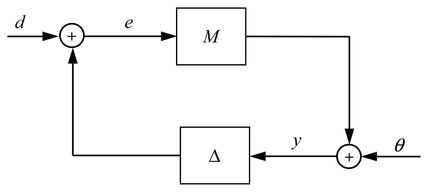
Suppose a nominal dynamics M is feedback-connected by an unstructured uncertainty Δ bounded by 2D-H_∞ norm, ||Δ||_∞ ≤γ⁻¹, as shown in Figure 1, then the closed-loop dynamics is guaranteed to be well-posed and internally stable if and only if ||M||_∞ < γ. This is named 2D Small Gain Theorem.

4. Robust Performance

Based on the 2D Small Gain theorem in Section 3, we will formulate in this section the sufficient and necessary condition of robust performance for the distributed control in mode-frequency domain.

Accommodating some extent of model uncertainties, the mode-frequency responses can be curve-fitted in the mode-Bode plot as a dense set:

$$\left\{G_0(1+W_1{\mathrm{\Delta }}_1):{\Vert {\mathrm{\Delta }}_1\Vert }_{\infty }\le 1\right\}.$$

(15)

Therein G₀ stands for a nominal plant:

$$G_0(\lambda ,s)=\frac{{\tau }_{0}s+1}{{\tau }_0{s}^2+s+\lambda },$$

(16)

where the nominal value of heat-diffusion relaxation τ₀ is assigned to be uniformly distributed. The 2D robustness weighting W₁ envelops all multiplicative perturbations W₁Δ₁ in the mode-Bode magnitude plot. As such, the dense set in Equation (15) contains all mode-frequency responses considered in real operation.

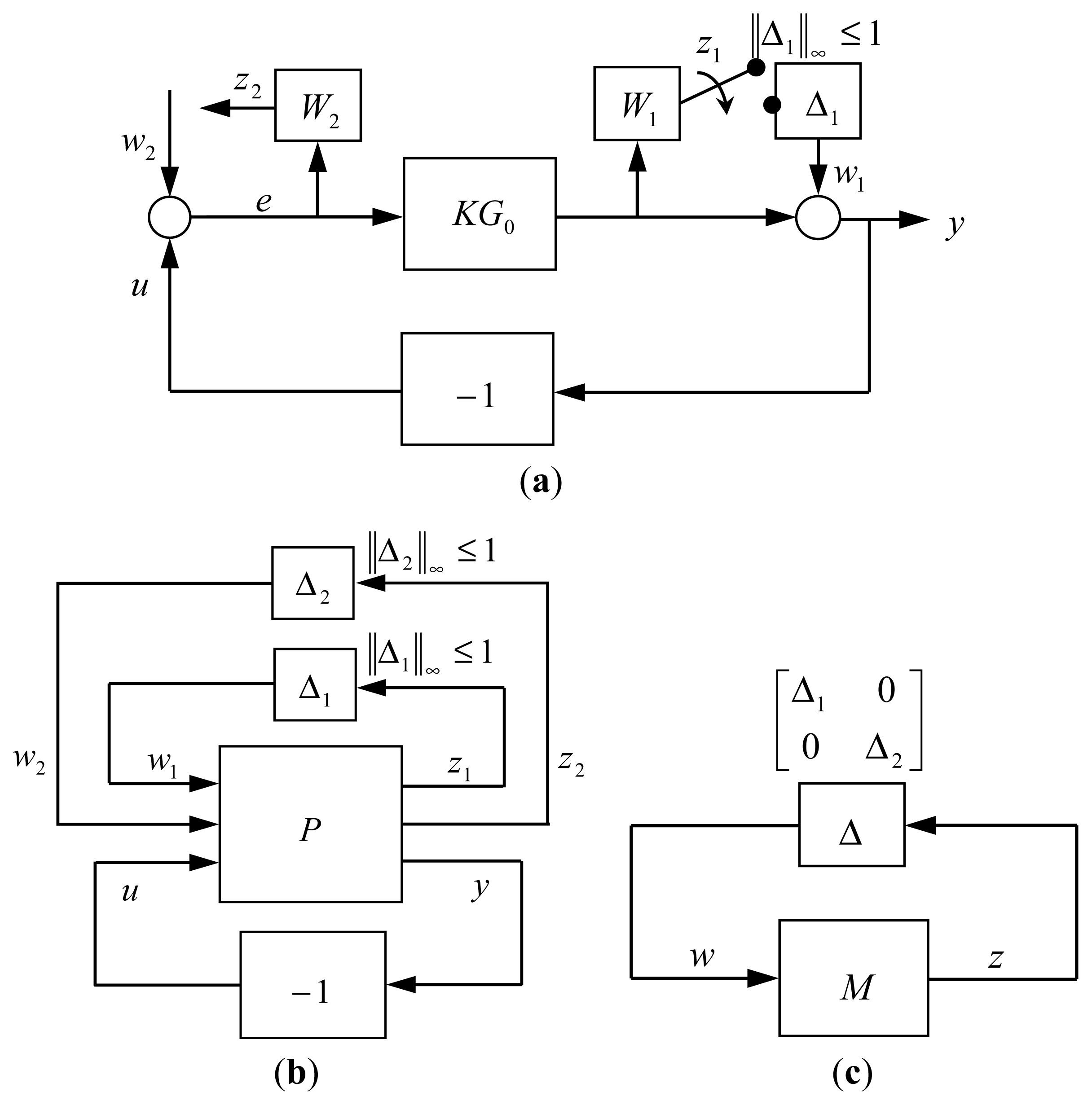
As shown in Figure 2a, the 2D controller K, pre- or post-composite to the plant, together with a negative unit feedback −1 executes the feedback compensation. The controller K is to guarantee specified performance for any member of the dense set in Equation (15), named Robust Performance. In L₂-gain control, the performance is specified by:

$${\int }_0^T{\int }_{\mathrm{\Omega }}C(x){\mid {\widehat{z}}_2(x,t)\mid }^{2}dx\hspace{0.17em}dt<{\gamma }^2{\int }_0^T{\int }_{\mathrm{\Omega }}C(x){\mid {\widehat{w}}_2(x,t)\mid }^{2}dx\hspace{0.17em}dt,\forall T\in [0,\infty ),$$

(17)

where the exogenous disturbances w₂ comprises the slow-time reference command and sensor noises of higher frequencies, and the tracking error e has been weighted by the performance weighting W₂, i.e., z₂ = W₂e.

Tracing the path of signal flow in Figure 2a, one can transform the interconnection of blocks in Figure 2a into the feedback-interconnection of three blocks:

$$\text{Generalized\hspace{0.17em}plant\hspace{0.17em}}P:\left[\begin{array}{r}{z}_1\\ z_2\\ y\end{array}\right]=\left[\begin{array}{ccc}0& W_{1}K{G}_0& W_{1}K{G}_0\\ 0& W_2& W_2\\ 1& K{G}_0& K{G}_0\end{array}\right]\hspace{0.17em}\left[\begin{array}{c}{w}_1\\ w_2\\ u\end{array}\right];$$

(18)

$$\text{External\hspace{0.17em}feedback}:u=-y;$$

(19)

$$\text{Internal\hspace{0.17em}feedback\hspace{0.17em}}1:w_1={\mathrm{\Delta }}_1{z}_1,{\Vert {\mathrm{\Delta }}_1\Vert }_{\infty }\le 1.$$

(20)

Therein the internal disturbance w₁ and stability variable z₁ are induced from modelling uncertainty Δ₁. Moreover, if we replace the L₂-gain performance in Equation (17) by an internal feedback such as:

$$\text{Internal\hspace{0.17em}feedback\hspace{0.17em}}2:w_2={\mathrm{\Delta }}_2{z}_2,{\Vert {\mathrm{\Delta }}_2\Vert }_{\infty }\le 1,$$

(21)

then the robust performance of the original setting in Figure 2a is equivalent to the robust stability of the closed-loop system in Figure 2b. This equivalency is inferred from 2D Small Gain theorem in conjunction with the equivalence of L₂-gain to 2D-H_∞ norm. Substituting Equation (19) into Equation (18) yields the lower fractional transformation of Figure 2b, as shown in Figure 2c. It becomes the feedback-interconnection of two blocks:

$$M=\left[\begin{array}{cc}-W_{1}T& W_{1}T\\ -W_{2}S& W_{2}S\end{array}\right]\mathrm{\hspace{0.17em} }\text{and\hspace{0.28em}}\mathrm{\Delta }=\left[\begin{array}{cc}{\mathrm{\Delta }}_1& 0\\ 0& {\mathrm{\Delta }}_2\end{array}\right];\hspace{0.17em}z=\left[\begin{array}{c}{z}_1\\ z_2\end{array}\right],\hspace{0.17em}w=\left[\begin{array}{c}{w}_1\\ w_2\end{array}\right],$$

(22)

where S is the sensitivity function 1/(1 + KG₀) and T is its complementary function, i.e., S +T =1. The first requirement of the controller K is to make the sensitivity function S asymptotically stable.

If the Δ-structured singular value μ_Δ is defined by:

$${\mu }_{\mathrm{\Delta }}(M)=\frac{1}{\text{min}\{\overline{\sigma }(\mathrm{\Delta }):\text{det}(I-M\mathrm{\Delta })=0\}},$$

(23)

then based on Nyquist criterion, the robust 2D-stability of Figure 2c is guaranteed, so is robust performance of Figure 2a, if and only if:

$${\mu }_{\mathrm{\Delta }}(M(\lambda ,j\omega ))\le 1,\text{for\hspace{0.17em}all\hspace{0.17em}}(\lambda ,\omega )\in \mathrm{\Lambda }\times {\mathfrak{R}}^{+}.$$

(24)

Substituting Equation (22) into Equation (23) yields:

$${\mu }_{\mathrm{\Delta }}(M)=\frac{1}{\text{min}\{\text{max}(\mid {\mathrm{\Delta }}_1\mid ,\mid {\mathrm{\Delta }}_2\mid ):1+W_{1}T{\mathrm{\Delta }}_1-W_{2}S{\mathrm{\Delta }}_2=0\}},$$

(25)

which, after careful calculation, is explicitly shown to be:

$${\mu }_{\mathrm{\Delta }}(M)=\mid W_{1}T\mid +\mid W_{2}S\mid .$$

(26)

Therefore, the set of sensitivity functions with robust performance is:

$$\left\{S:\mid W_1(\lambda ,j\omega )(1-S(\lambda ,j\omega ))\mid +\mid W_2(\lambda ,j\omega )S(\lambda ,j\omega )\mid <1,\forall (\lambda ,\omega )\in \mathrm{\Lambda }\times {\mathfrak{R}}^{+}\right\}.$$

(27)

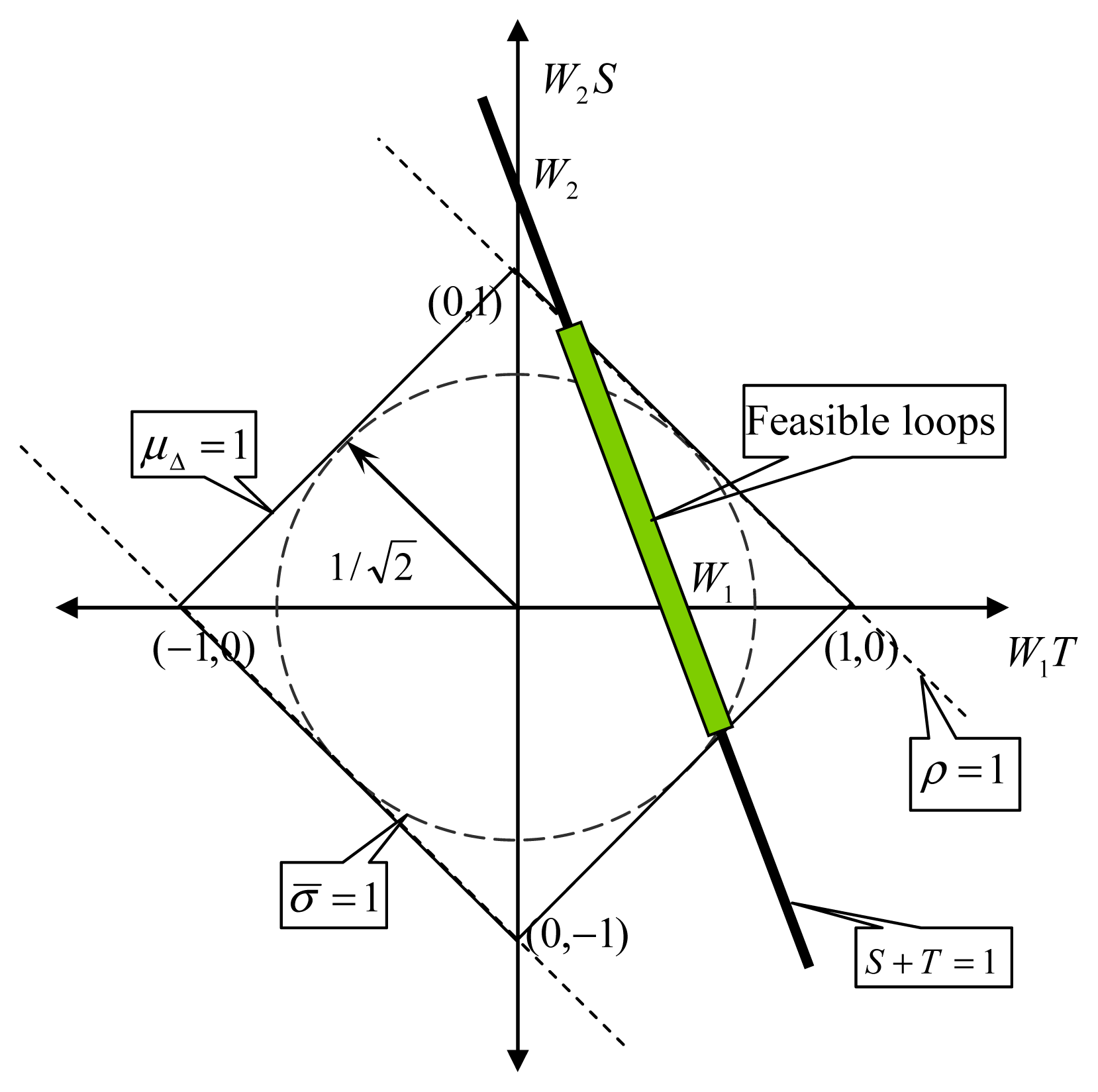
Finally, we know that any feasible loop S is a stable transfer-function and a member of Equation (27). A graphical interpretation of robust performance is shown in Figure 3, where the line segment of S +T = 1 inside the diamond of μ_Δ (M) =1 represents the set of all feasible loops S. In Figure 3, we also demonstrate the conservatism of singular value σ̄ (M) and the risk of spectral radius ρ (M) as metrics of robust performance. In fact, nD state-space robust control syntheses in the control literature always takes the singular value σ̄ (M) as the metric of robust performance, therefore ensuring conservatism when numerically solving distributed control.

5. 2D-μ Manifolds

The set of feasible loops S ’s at a fixed (λ, ω ):

$$\left\{S:\mid W_1(1-S)\mid +\mid W_{2}S\mid <1\right\},$$

(28)

as shown in Equation (27), is an open, convex and complex-valued set. It appears as a plate in the Cartesian plane coordinated by Re(S) and Im(S), named μ-plate at (λ, ω ). The μ-plate is attributed to the following geometry:

(P1)

Every μ-plate is symmetric to the Re(S) axis.

(P2)

If |W₁| ≥ |W₂| and both are not greater than 1, the μ-plate is contained in the ellipse that has focuses (0,0) and (1,0), major-axis length 1/|W₂|, and minor-axis length $\sqrt{1-{\mid W_2\mid }^2}/\mid W_2\mid$.

(P3)

If |W₂| ≥ |W₁| and both are not greater than 1, the μ -plate is contained in the ellipse that has focuses (0,0) and (1,0), major-axis length 1/|W₁|, and minor-axis $\sqrt{1-{\mid W_1\mid }^2}/\mid W_1\mid$.

(P4)

If |W₁| = |W₂| <1, the boundary of the μ-plate is just the ellipse described in (P2) or (P3).

(P5)

If |W₁| = |W₂| ≈ 1, the μ-plate degenerates into a line segment between (0,0) and (1,0).

(P6)

If |W₁| >> |W₂|, the boundary of μ-plate is close to a circle of radius 1/|W₁| centered at (1,0).

(P7)

If |W₂| >> |W₁|, the boundary of (W₁, W₂ ) is close to a circle of radius 1/|W₂| centered at (0,0).

(P8)

For |W₁| and |W₂| being both greater than 1, the μ-plate degenerates into disappearance.

The geometry of μ-plates reflects some trade-off principles in feedback design as follows. Firstly, a μ-plate tends to disappear as the robustness weighting W₁ and the performance weighting W₂ are simultaneously magnified. This reflects the trade-off between robust stability and nominal performance. Secondly, the uncertain perturbation W₁Δ₁ arising from insufficient information of thermal inductance is distributed in high-frequency domain, so W₁ is high-passed. Thus W₂ allows only for low-pass, meaning that the closed-loop system is unable to guarantee tracking of fast-time reference temperatures to some extent. This reflects the trade-off between system maneuverability and information insufficiency. Thirdly, for large W₁ and W₂, high-gain controller can diminish the sensitivity function to achieve feasibility in Equation (27), which requires powerful heater/cooler and high-bandwidth, low-noises thermal couplers. This reflects the trade-off between hardware cost-down and robust performance.

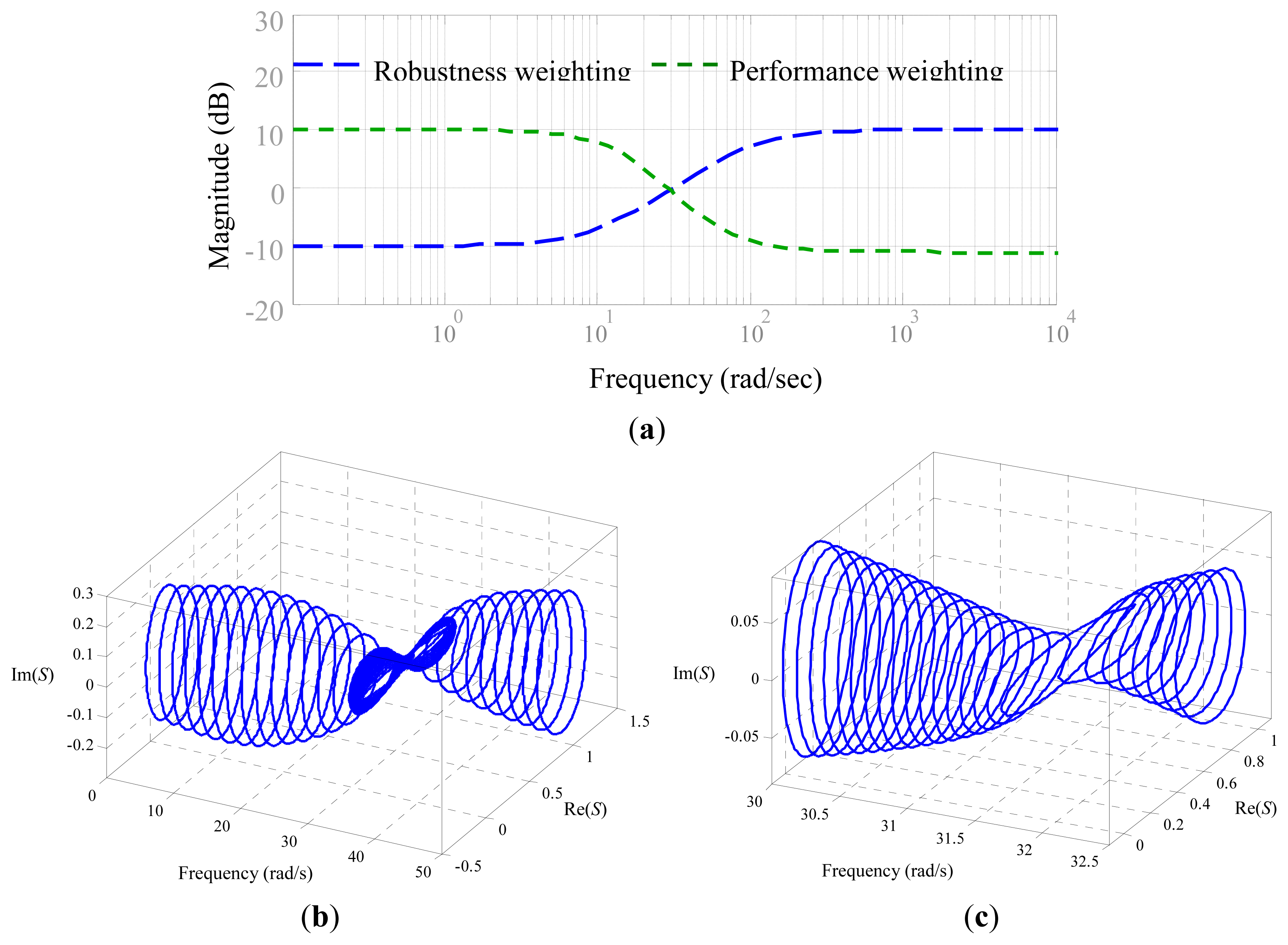
The union of all μ-plates for all ω ∈ℜ⁺ at fixed λ becomes a manifold, named by λ-mode μ-manifold. For a graphical manifestation of the μ-plate geometry, here is plotted the μ-manifold of some λ-mode for weighting functions (W₁, W₂) shown in Figure 4a. Figure 4b shows the appearance of (λ-mode) μ-manifold that corresponds to the properties (P1)–(P8). For example, this μ-manifold has a narrow tunnel at frequency ω = 31.5 at which both W₁ and W₂ have magnitudes close to one, as indicated by (P5), the close view of which is shown in Figure 4c.

The controller K is proposed to take the form:

$$K(\lambda ,s)=K_0(\lambda ,s)\frac{{\tau }_0{s}^2+s+\lambda }{{\tau }_{0}s+1},$$

(29)

where the temporal order of K₀ is larger than that of the nominator at least by one for a physically existent dynamics K. With the help of the μ-manifold’s topology, we expand 1D loopshaping technique on 2D loopshaping in mode-frequency domain to synthesize all feasible K₀’s. After the identification of 2D performance weighting W₂ and robust weighting W₁, every feasible controller K has to guarantee that every λ-mode sensitivity function map a line inside the λ-mode μ-manifold for all λ ∈Λ. In the sequel, we demonstrate the procedure of 2D-μ loopshaping for non-Fourier heat conduction in longitudinal direction.

6. 2D-μ Loopshaping

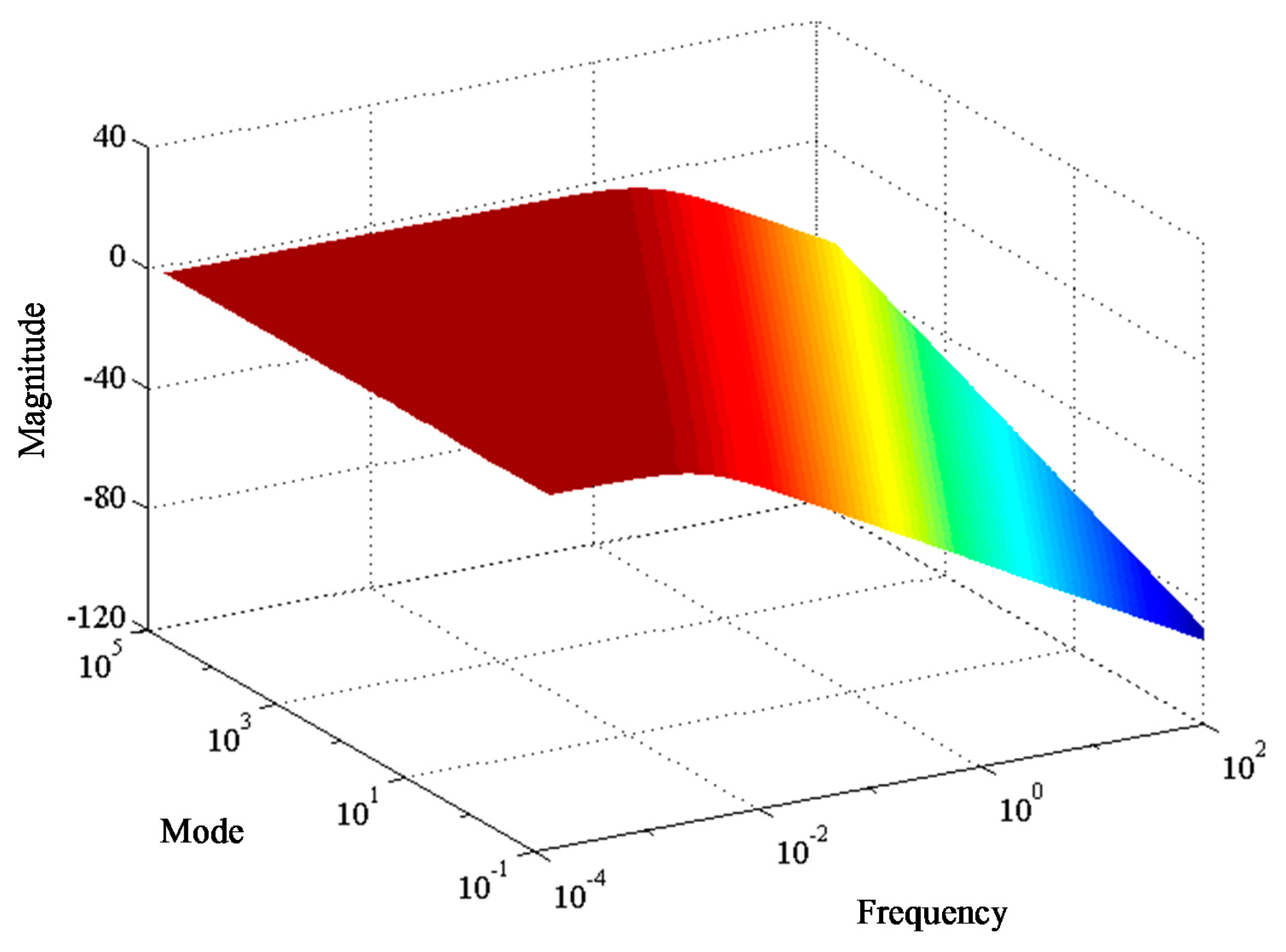
As shown in Section 2, the 2D transfer-function G of non-Fourier heat conduction is:

$$G(s,\lambda )=\frac{\tau s+1}{\tau s^2+s+\lambda },$$

(30)

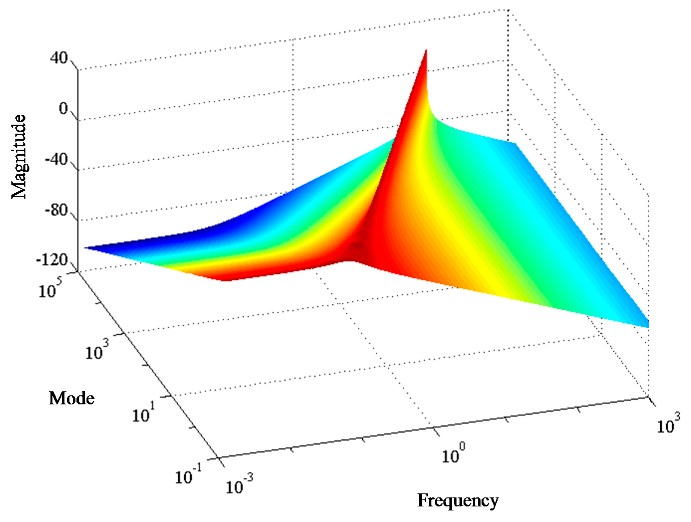
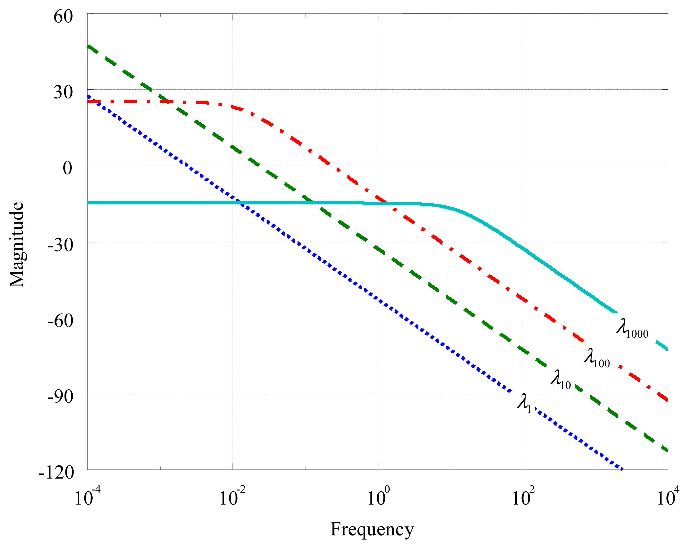
the typical mode-frequency response of which is shown in Figure 5 as the modal-Bode magnitude plot. Figure 5 shows that non-Fourier heat conduction in a small region behaves like a standing wave, wherein larger (smaller) modes are of higher (lower) resonant frequencies.

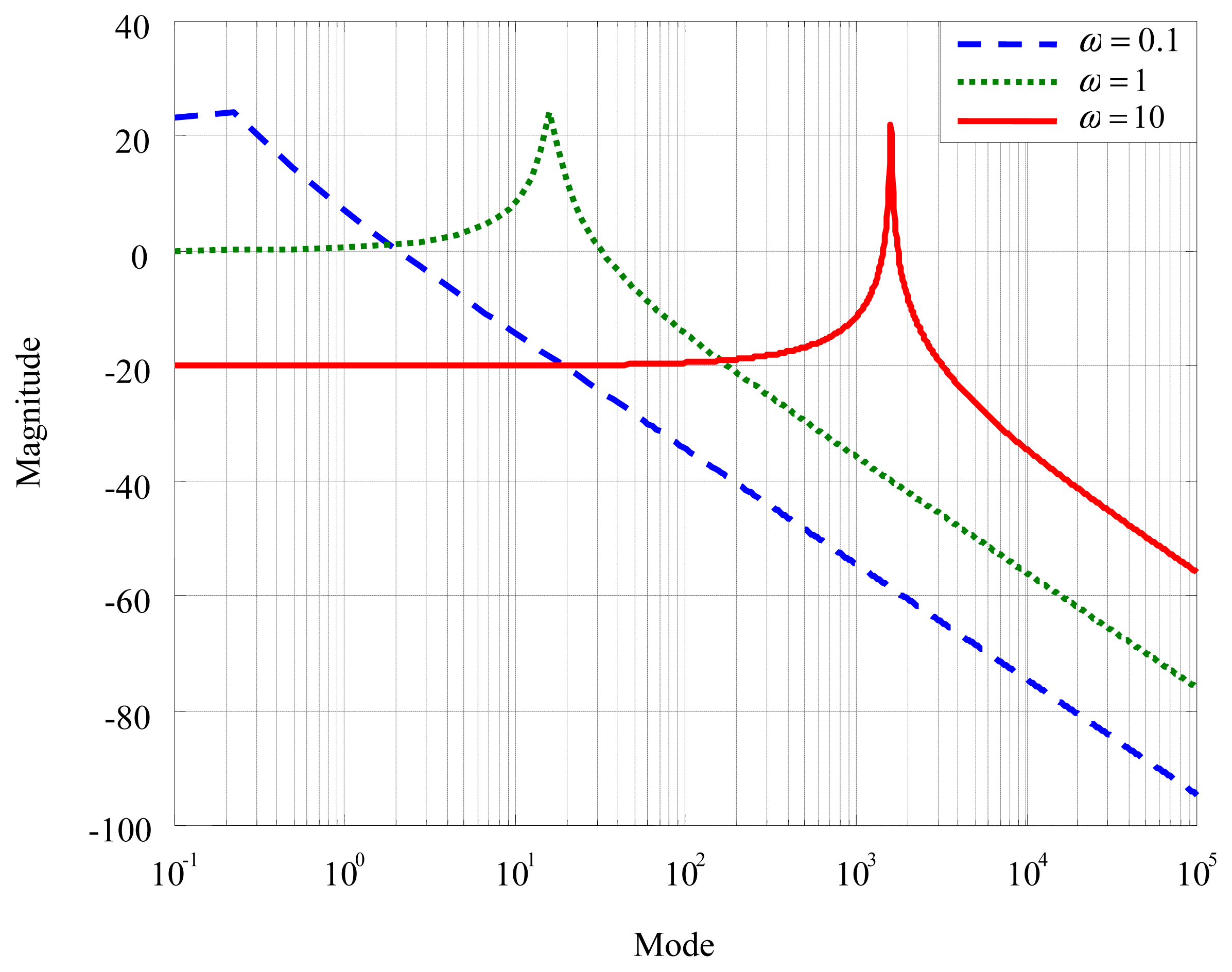
That is, with pointed control, slower heating is able to result in moderate transience, but is unable to track subtle distribution of temperature in space. On the other hand, to track a spatial distribution with larger variation, fast heating has to be adopted, but it results in severe overshoot and rising time that could burn organic materials. Figure 6 shows the mode responses at different frequencies, which provides a clearer vision of this phenomenon, wherein the mode responses at different frequencies have similar patterns to the frequency responses at different modes. This similarity prevents point control from reaching required temporal and spatial responses at the same time. To track precise local-temperatures and suppress the transience simultaneously, distributed control has to be developed.

In this section, the 2D-μ loopshaping in mode-frequency domain is developed to synthesize 2D transfer-function controllers served for distributed control. The 2D-μ loopshaping consists of two main steps as follows:

Step 1. Construction of Generalized Plant

Consider that modelling uncertainties result from non-uniform distribution of the relaxation time τ. Let the dense set of plants:

$$\left\{G_0(1+W_1{\mathrm{\Delta }}_1):{\Vert {\mathrm{\Delta }}_1\Vert }_{\infty }\le 1\right\}$$

(31)

contain the set of mode-frequency responses accommodating empirical extent of the uncertainty, wherein G₀ stands for the nominal plant:

$$G_0(\lambda ,s)=\frac{{\tau }_{0}s+1}{{\tau }_0{s}^2+s+\lambda }.$$

(32)

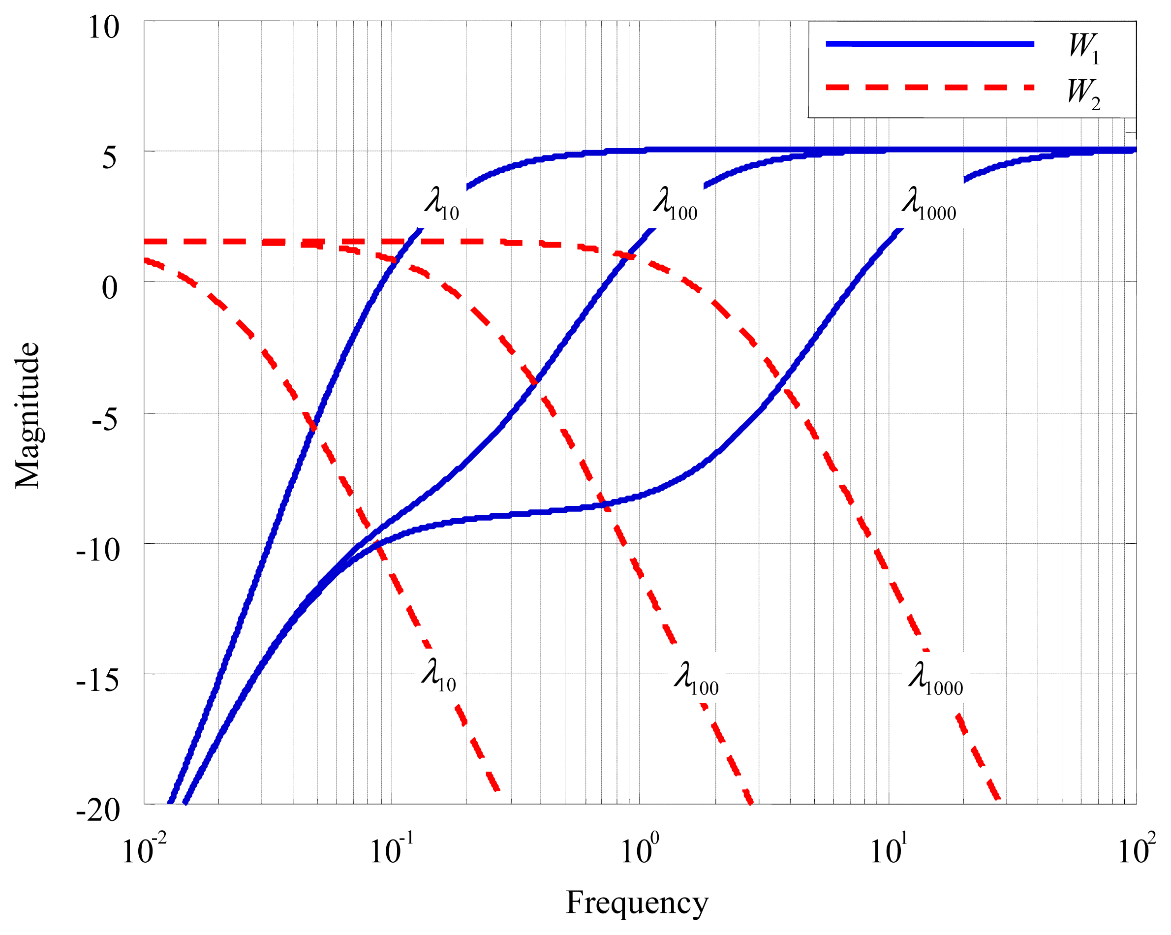
In Equation (31), Δ₁ (λ, jω) accounts for the phase uncertainty for each mode, and the magnitude of the perturbation is specified by the 2D robustness weighting W₁. The perturbation satisfies:

$$\left|\frac{G(\lambda ,j\omega )}{G_0(\lambda ,j\omega )}-1\right|\le \mid W_1(\lambda ,j\omega )\mid ,\forall (\lambda ,\omega )\in \mathrm{\Lambda }\times {\mathfrak{R}}^{+}$$

(33)

with a preset range of τ, so the 2D robustness weighting W₁ is chosen as the envelop of all multiplicative perturbations W₁ Δ₁ in the modal-Bode magnitude plot. By this way, a 2D robustness weighting W₁ can be curve-fitted out of mode-frequency responses, as shown in Figure 7.

For τ ∈[4.5, 20], it is chosen as:

$$W_1(\lambda ,s)=\frac{1.8s\left(s+0.01{\lambda }^{½}\right)}{\left(s+0.05\right)\left(s+0.05{\lambda }^{½}\right)}(\lambda \in {\mathfrak{R}}^{+}).$$

(34)

As for the 2D performance weighting W₂, it has to satisfy two requirements: (i) following the 2D-μ manifold’s rules (P5)–(P8) in Section 5 to guarantee feasibility; and (ii) being of high-pass in space and of low-pass in time to achieve the required performance- suppress temporally abrupt transience and simultaneously track subtle temperature distribution in space. Thereby, the 2D performance weighting W₂ is chosen as:

$$W_2(\lambda ,s)=\frac{0.012{\lambda }^{½}}{s+0.01{\lambda }^{½}}(\lambda \in {\mathfrak{R}}^{+}).$$

(35)

Figure 8 shows the 2D performance weighting W₂ in the modal-Bode plot and Figure 7 shows its projection onto the mode axis, which demonstrates the requirement (ii).

Step 2. Loopshaping Based on 2D-μ Manifold’s Rules

Based on the principle of 1D-μ loopshaping in [35] and 2D-μ manifolds rules in Section 5, every loop gain L of the closed-loop at each mode should satisfy:

$$\mid L\mid >\frac{\mid W_2\mid }{1-\mid W_1\mid }\hspace{0.17em}\text{where\hspace{0.17em}}\mid W_2\mid >>1>\mid W_1\mid ,\text{and\hspace{0.17em}}\mid L\mid <\frac{1-\mid W_2\mid }{\mid W_1\mid }\hspace{0.17em}\text{where\hspace{0.17em}}\mid W_2\mid <1<<\mid W_1\mid .$$

(36)

Accordingly, we plot two curves in Bode magnitude plot: first, the graph of |W₂|/(1−|| W₁||) over the low-frequency range where |W₂| > 1 > |W₁|; second, the graph of (1− |W₂|) /|W₁| over the high-frequency range where |W₁| > 1 > |W₂|. Then, the graph of |L| lies above the first graph at low frequency and below the second curve at high frequency. Let it roll off at least as fast as does |G₀| at very high frequency and do a smooth transition from low to high frequency, keeping the slope as gentle as possible near crossover, the frequency where the magnitude equals 1, to force the sensitivity function to lie inside the μ-manifold.

By this way, the 2D loop-gain L is synthesized to be:

$$L(\lambda ,s)=\frac{0.01{\lambda }^{½}}{s+0.01{\lambda }^{³/₂}},$$

(37)

which is shown in Figure 9. The 2D transfer-function controller K achieving robust performance becomes:

$$K(\lambda ,s)=\frac{0.01{\lambda }^{½}}{s+0.01{\lambda }^{³/₂}}\frac{{\tau }_0{s}^2+s+\lambda }{{\tau }_{0}s+1},$$

(38)

which is designed to be proper not only in time but also in space on purpose of dealing with spatially discontinuous inputs.

Figure 10 plots the graph of |W₁ (1−S)| + |W₂S|, which is not larger than 1 for all modes, indicating the feasibility of the controller K. Finally we check the reliability of the controller K in achieving robust performance by the distance of the sensitivity function to the boundary of the μ-manifold. Figure 11 partly shows the reliability by plotting the sensitivity function lying inside the μ -manifold at λ₁₀₀.

7. Implementation of 2D Transfer-Functions Controllers

Let a general 2D transfer-function controller K be spatiotemporally discretized into some state-space realization:

$$\begin{array}{l}{v}_{k+1}=\mathrm{\Phi }{v}_k+\mathrm{\Gamma }{e}_k\\ u_k=\mathcal{C}{v}_k+\mathcal{D}{e}_k,\end{array}$$

(39)

for on-line signal processing in an embedded controller or for computer simulation.

Referring to Figure 12. Suppose there are n state variables in Step 3, p analog pins in the distributed temperature transducer and m metal contacts in the distributed heater. The microcontroller array comprises d dsPICs; each of them provides multi-channeled ADC converter, multi-channeled PWM generators and CAN bus protocol in peripheral, and DSP engine in CPU. With this dsPIC array, the plant output is divided into p / d channels and the plant input into m/ d channels. The state x is then stacked up by n / d columns, x_i ∈ ℜ ^n/d, i = 1,2, · · ·, d. Accordingly, the system matrices (Φ, Γ, , ) are partitioned into d × d blocks, where:

$${\mathrm{\Phi }}_{ij}\in {\mathfrak{R}}^{n/d\times n/d},{\mathrm{\Gamma }}_{ij}\in {\mathfrak{R}}^{n/d\times p/d},{\mathcal{C}}_{ij}\in {\mathfrak{R}}^{m/d\times n/d},\text{and\hspace{0.17em}}{\mathcal{D}}_{ij}\in {\mathfrak{R}}^{m/d\times p/d}.$$

(40)

Each i th dsPIC for i = 1,2, · · ·, d stores the i th column of present state x_i in RAM, has the matrices {(Φ_ij, Γ_ij, _ij, _ij ) : j =1,2, · · ·, d } as parameters in ROM, and performs the computing as:

$$u_i=\sum _{j=1}^d{\mathcal{C}}_{ij}{v}_j+{\mathcal{D}}_{ij}{e}_j;v_i=\sum _{j=1}^d{\mathrm{\Phi }}_{ij}{v}_j+{\mathrm{\Gamma }}_{ij}{e}_j,i=1,2,\cdots ,d$$

(41)

to update state and decide control signals, where e stands for the distributed tracking error. The present states and sampled inputs distributed in the dsPIC array communicate with the built-in CAN bus peripherals. Most importantly, the Timer peripheral in every microcontroller sends interruption signals at a fixed time identical to the sampling time T set at the stage of computer simulation to let microcontrollers’ CPUs execute the DSP routines. In each Timer-interruption routine, temperatures in the distribution are sampled, the present states and measurements are communicated among microcontrollers, cloud matrix-iterated computation of Equation (41) updates the distributed states, and PWM outputs are sent to the distributed driver of the heating contacts. Such an interruption design is to guarantee that the controller under implementation is identical to that in the computer simulation. The distributed driver of the heater is an array of high-frequency switching buck choppers.

For digital implementation of 2D transfer-function controllers with the above Cloud Matrix Iteration Time-fixed DSP program (MIT) on microcontroller array, there are the following exclusive merits:

(1)

We avoid a mechanical scanner for data acquisition and control output, which shortens sampling time to boost real-time fashion;

(2)

Distributed computing replaces one generous-purpose microprocessor auxiliary with microcontrollers functioning DAC, PWM, and communication, therefore dramatically reducing the cost of controller manufacture without sacrificing performance; and

(3)

The microcontroller array consists of the same dsPICs, which shortens the time for code development.

8. Numerical and Experimental Study

This section presents numerical and experimental investigation on the performance of the 2D transfer-function controllers that are synthesized with Section 6 and implemented by Section 7. We will scrutinize whether the final design is capable of suppressing temporally transience and simultaneously track temperature distribution of highly spatial resolution.

Here hotdog meat is chosen as the heat-conduction material of uniform thermal parameters in the longitudinal direction. The non-Fourier heat conduction is belonging to hyperbolic dynamics:

$$\tau \frac{{\partial }^2\psi }{\partial t^2}+\frac{\partial \psi }{\partial t}-\frac{k}{C}\frac{{\partial }^2\psi }{\partial x^2}=\tau \frac{\partial u}{\partial t}+u\mathrm{\hspace{0.17em} }x\in [0,\ell ],\psi =0\mathrm{\hspace{0.17em} }\text{at\hspace{0.28em}}x=0,\ell .$$

(42)

Therein, the meat is of length ℓ = 5 mm, thermal conductivity is k = 0.8W m· K, mass density ρ = 1230 kg/m³, thermal capacitance at constant volume C_v = 4.66 kJ/kg · K, and relaxing time τ =16 s. Accordingly, the 2D transfer-function of the plant is:

$$G(s,\lambda )=\frac{\tau s+1}{\tau s^2+s+\lambda }.$$

(43)

During control synthesis with 2D-μ loopshaping in mode-frequency domain, we assume that modelling uncertainties arise from the parametric error of relaxing time τ ∈[4.5,20], and the robust weighting is identified as above to be:

$$W_1(\lambda ,s)=\frac{1.8s\left(s+0.01{\lambda }^{½}\right)}{\left(s+0.05\right)\left(s+0.05{\lambda }^{½}\right)}.$$

(44)

As for the performance weighting W₂, three cases are investigated:

• Case 1: W₂ (λ, s ) = 1.2 that is spatiotemporally uniform;
• Case 2: $W_2(\lambda ,s)=\frac{0.012}{s+0.01}$ that is spatially uniform and temporally low-passed; and
• Case 3: $W_2(\lambda ,s)=\frac{0.012{\lambda }^{½}}{s+0.01{\lambda }^{½}}$ that is spatially high-passed and temporally low-passed.

Following the procedures of 2D-μ loopshaping in Section 6, three 2D transfer-function controllers for these cases are calculated for comparison of their performances.

The performance setup is to track pulse-width-modulated (PWM) temperature distribution, which is discontinuous in space. Here the temperature under tracking is uniformly distributed in ℓ/4 ≤ x ≤ ℓ/2. This kind of performance is needed for heat treatment in removing a tumor. Figure 13 shows the temperature distributions at steady state for three cases. Only Case 3 arrives at the requirement of precisely tracking the local temperatures in high resolution. Figure 14 shows the temporal responses at x = 2ℓ/5 of three cases, wherein only Case 3 suppresses the overshoot that otherwise could damage the meat under operation. The spatiotemporal response of Case 3 is recorded in Figure 15 that demonstrates temperature snapshots evolved into the command temperature from the initial.

With these results, we verify the principle that distributed control of proper design is able to decouple temporal requirement from spatial requirement of the closed-loop performance. That is, temporal evolution and spatial distribution can be independently setup with distributed control technique developed in this paper.

9. Recapitulation

Via this paper, we work on the following issues about the distributed control of heat conduction in thermally inductive materials:

(1)

Verify the principle that, beyond the capability of pointed control, distributed control can simultaneously track the spatial distributions and temporal transients, which has overwhelming advantages in thermally inductive materials of modern days.

(2)

Extend the classical control to 2D version for non-Fourier heat conduction.

(3)

Implement the 2D transfer-function controller into the microcontroller array with cloud technology.

(4)

Develop 2D-μ loopshaping in mode-frequency domain for the synthesis of 2D transfer-function controllers.