Multiscale Compression Entropy of Microvascular Blood FlowSignals: Comparison of Results from Laser Speckle Contrastand Laser Doppler Flowmetry Data in Healthy Subjects


Abstract
: Microvascular perfusion is commonly used to study the peripheral cardiovascular system. Microvascular blood flow can be continuously and non-invasively monitored with laser speckle contrast imaging (LSCI) or with laser Doppler flowmetry (LDF). These two optical-based techniques give perfusion values in arbitrary units. Our goal is to better understand the perfusion time series given by each technique. For this purpose, we propose a nonlinear complexity analysis of LSCI and LDF time series recorded simultaneously in nine healthy subjects. This is performed through the computation of their multiscale compression entropy. The results obtained with LSCI time series computed from different regions of interest (ROI) sizes are examined. Our findings show that, for LSCI and LDF time series, compression entropy values are less than one for all of the scales analyzed. This suggests that, for all scales, there are repetitive structures within the data fluctuations. Moreover, at the largest scales studied, LDF signals seem to have structures that are different from those of Gaussian white noise. By opposition, this is not observed for LSCI time series computed from small ROI sizes.1. Introduction
Analysis of the microvascular perfusion presents a particular challenge in cardiovascular studies because, for pathologies, such as diabetes or hypertension, microcirculation is affected long before organ dysfunctions become clinically manifest (see, e.g., [1–3]). However, perfusion can exhibit high variability over time [4]. Therefore, a continuous monitoring of microvascular perfusion has become of clinical interest. For this purpose, several optical-based techniques have been developed [5]. Among them, laser Doppler flowmetry (LDF) [6] and laser speckle contrast imaging (LSCI) [7] are commercially-available modalities that have the advantage of leading to real-time perfusion data [8].
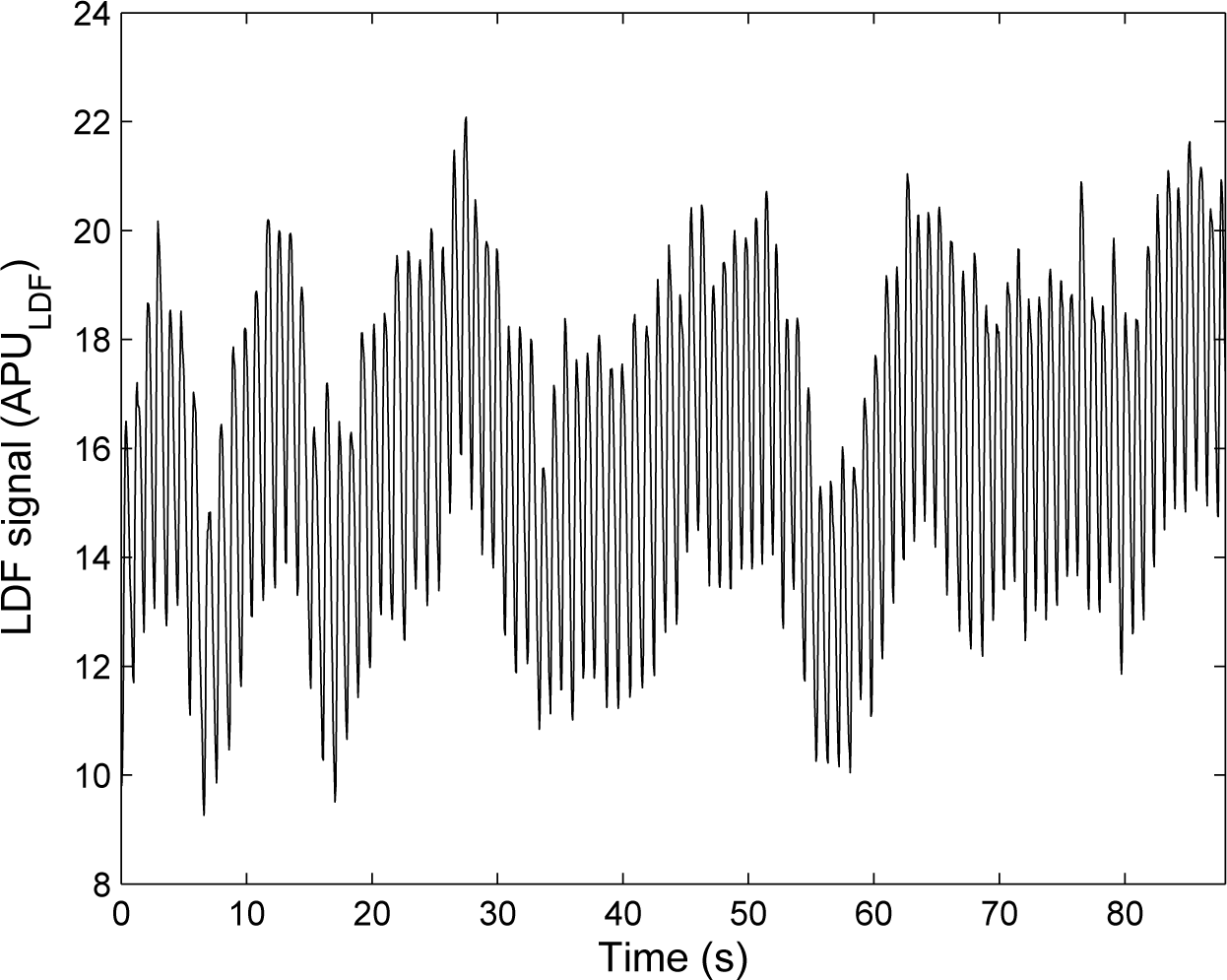
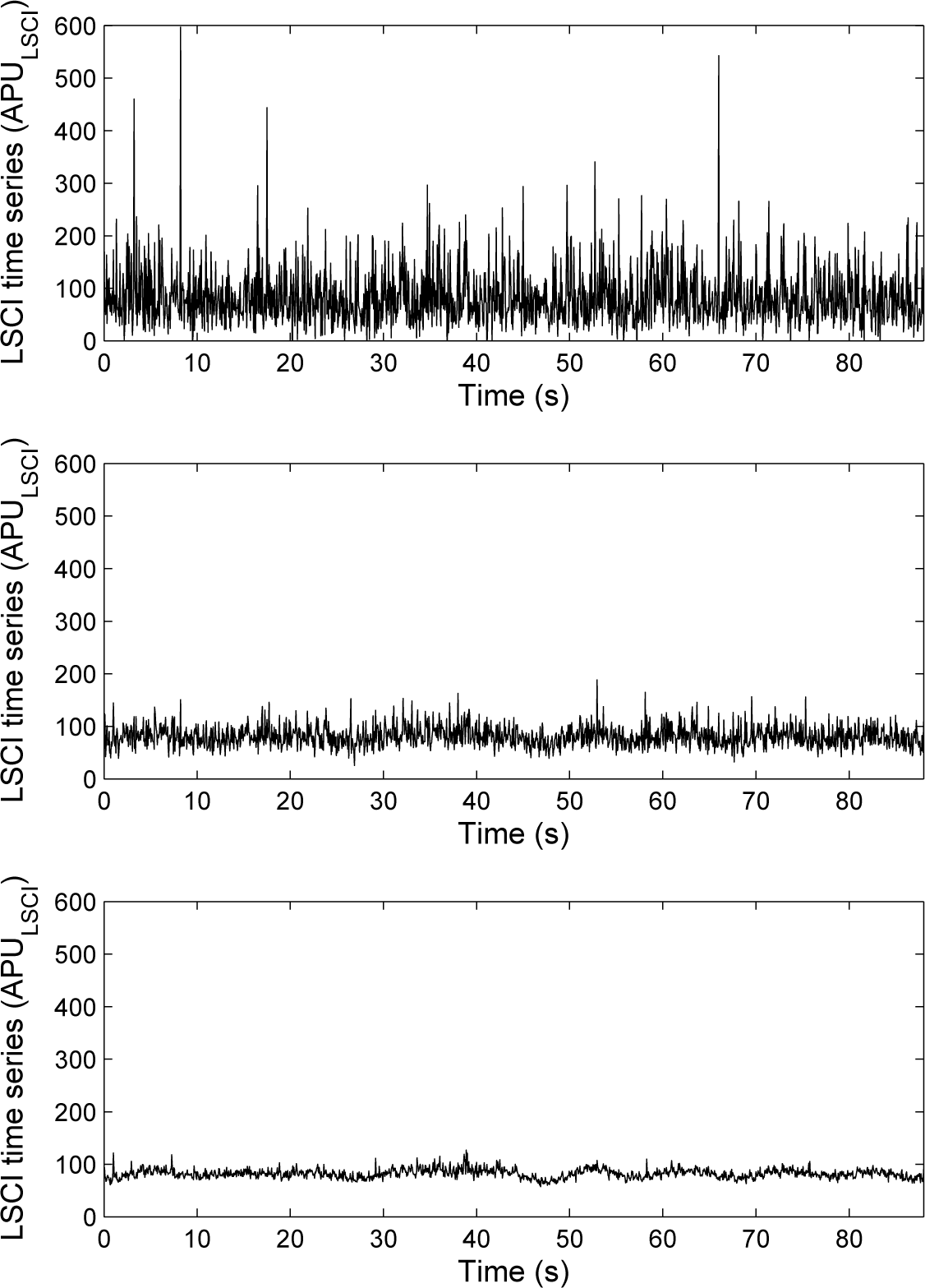
LDF was introduced in the 1970s [6] and has now a well-established theory [9]. In LDF, the tissue under study (skin, for example) is illuminated with a low-power laser light through a probe containing optical fiber light guides. One optical fiber leads the light to the tissue, and a second optical fiber collects the backscattered light that is transmitted to a photodetector. LDF relies on the Doppler frequency shift that appears when light is scattered by moving blood cells of the microcirculation. The LDF perfusion is defined as the first moment of the power spectrum of the photocurrent fluctuations. An example of an LDF signal recorded at rest is shown in Figure 1. At the beginning, LDF was a single-point measurement technique. However, because of the spatially inhomogeneous structure of the microcirculation, laser Doppler imagers (scanning imagers) were introduced in the early 1990s [10,11]. Full-field laser Doppler instruments have more recently been proposed and are still the object of recent research [12].
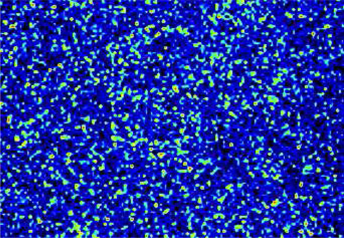
LSCI is another recent and full-field technique to monitor microvascular blood flow. LSCI relies on the wide-field illumination of a tissue with a laser light [7,13,14]. In the tissue, some of the photons scatter dynamically from moving blood cells. Because of the motions of the moving blood cells in the illuminated tissue, a dynamic speckled image is obtained on the detector that is a camera. When the exposure time of the camera is longer than the time scale of the speckle intensity fluctuations (typically less than 1 ms for biological tissues), the camera integrates the intensity variations, which results in a blurring of the speckle pattern. The degree of blurring is quantified by the speckle contrast K, which is calculated as:
In order to better understand LDF signals and to extract physiological information from the data, LDF time series have been the subject of many works, such as wavelet-based or entropy-based studies (see e.g., [17–22]). By opposition, and probably because laser speckle contrast imagers have been commercialized only recently, LSCI data have been the subject of very few analyses [23]. Moreover, as both LDF and LSCI give perfusion values in arbitrary units, works aiming at comparing the results given by the two techniques have become necessary [24–27]. Thus, it has been reported that LSCI and LDF do not probe the same volume of tissue [28]: the penetration depth of LSCI is lower than the one of LDF for similar wavelengths. Moreover, the possible linearity between the perfusion values given by the two techniques has also been studied [29]. However, other comparisons between LDF and LSCI perfusion values are needed. Furthermore, works aiming at better understanding laser speckle contrast images are also necessary.
Our goal herein is two-fold: (i) to better understand LSCI through an investigation of LSCI time series complexity on multiple time scales; for this purpose, an algorithmic information theory-based concept relying on a coarse-graining procedure and a data compressor is applied on LSCI time series (multiscale compression entropy); (ii) to compare the multiscale compression entropy of LSCI data with the one of LDF signals; For this purpose, our framework is also applied on LDF signals recorded simultaneously to laser speckle contrast images.
2. Materials and Methods
2.1. Measurement Procedure
The measurement procedure was performed in nine healthy subjects between 20 and 41 years old who provided written, informed consent prior to participation. The study was carried out in accordance with the Declaration of Helsinki.
For each subject, LSCI and LDF data were recorded simultaneously on the dorsal face of the right forearm. For this purpose, a PeriCam PSI System (Perimed, Sweden) having a laser wavelength of 785 nm and an exposure time of 6 ms was used to record LSCI data. The distance between the laser head to skin was set around 15 cm [30]. This gave images with a resolution of 0.4 mm. LSCI data were recorded with a sampling frequency of 18 Hz in arbitrary laser speckle perfusion units (APULSCI). Moreover, a laser Doppler flowmeter having a 780-nm wavelength (PeriFlux System 5000, Perimed, Sweden) was used to acquire LDF signals. The LDF probe was positioned directly on the forearm. LDF perfusion values were assessed in arbitrary laser Doppler perfusion units (APULDF) and recorded on a computer via an analog-to-digital converter (Biopac System) with a sampling frequency of 20 Hz. A sub-sampling to 18 Hz was then performed.
In what follows and for each subject, 1,600 laser speckle contrast images and 1,600 LDF samples recorded simultaneously are processed. For each subject, a pixel was randomly chosen in the first laser speckle contrast image of the image sequence. This pixel was followed with time to obtain a time series of 1,600 samples. Moreover, around each pixel chosen above, square regions of interest (ROI) of a size of 3 × 3 pixels2 (1.44 mm2) and 15 × 15 pixels2 (36 mm2) were determined [26,31,32]. For each ROI, the mean of the pixel values (in APULSCI) inside the ROI was computed and followed on each image of the sequence to obtain a time-evolution signal (see Figure 3). For each subject, we therefore had three time series from LSCI data: one from a ROI of size of 1 × 1 pixels2, another from a ROI of size of 3 × 3 pixels2 and a third one from a ROI of size of 15 × 15 pixels2, as well as one time series from the LDF signal. Each of these time series were processed to compute their multiscale compression entropy.
2.2. Compression Entropy
From algorithmic information theory, the smallest algorithm that produces a string is the entropy of that string (Chaitin–Kolmogorov entropy) [33]. However, the development of such an algorithm is theoretically impossible, but data compression techniques might provide a good approximation. If the length of the text to be compressed is sufficiently large and if the source is an ergodic process, the ratio of compressed text to original text length represents the compression entropy per symbol. Based on this, we propose to assess the entropy of LSCI and LDF time series through their compressibility [34]. For this purpose, a modified version of the original LZ77 algorithm for lossless data compression introduced by Ziv and Lempel [35] is used.
The main steps of our algorithm, when applied on a time series s = {s1,…, sL}, are the following (in what follows, a subsequence (sm, sm+1,…, sn) of s is noted sm→n) [34]:
choose a sliding window size w and a lookahead buffer size b;
encode the first w elements of the time series without compression;
set a pointer p = w + 1;
for 1 ≤ v ≤ w, find the largest n (1 ≤ n ≤ b), such that sp→p+n−1 = sp−w+v→p−w+v+n−1;
encode the integers n and v into unary-binary code and the value of xp+n without compression;
set the pointer p to p = n + 1 and iterate to Step 4, till the end of the time series.
Therefore, compression entropy gives an indication to which degree the time series under study can be compressed using the detection of recurring sequences. The more frequent the occurrences of sequences (and thus, the more regular the time series), the higher the compression rate. The ratio of the lengths of compressed to uncompressed time series is used as a complexity measure and identified as compression entropy. Compared to Shannon entropy, compression entropy has the advantage of considering order within the sequence under study. Moreover, in contrast to the Shannon formula, the compression entropy takes the previous values of the system output into account.
In our work, different values for the sliding window size w and the lookahead buffer size b have been tested: 1 ≤ w ≤ 20 and 1 ≤ b ≤ 10 [34]. Moreover, for all of our time series, a normalization was performed before the compression entropy computation (subtraction of the mean and division by the standard deviation).
2.3. Multiple Time Scales Compression Entropy
In our work, we propose to compute compression entropy on multiple time scales. For this purpose, a coarse-graining procedure is used [36]: the original time series {s1,…, si,…, sL} is divided into non-overlapping windows of length τ, and the values of the data points inside each window are averaged, as:
3. Results
3.1. Results on LSCI Time Series
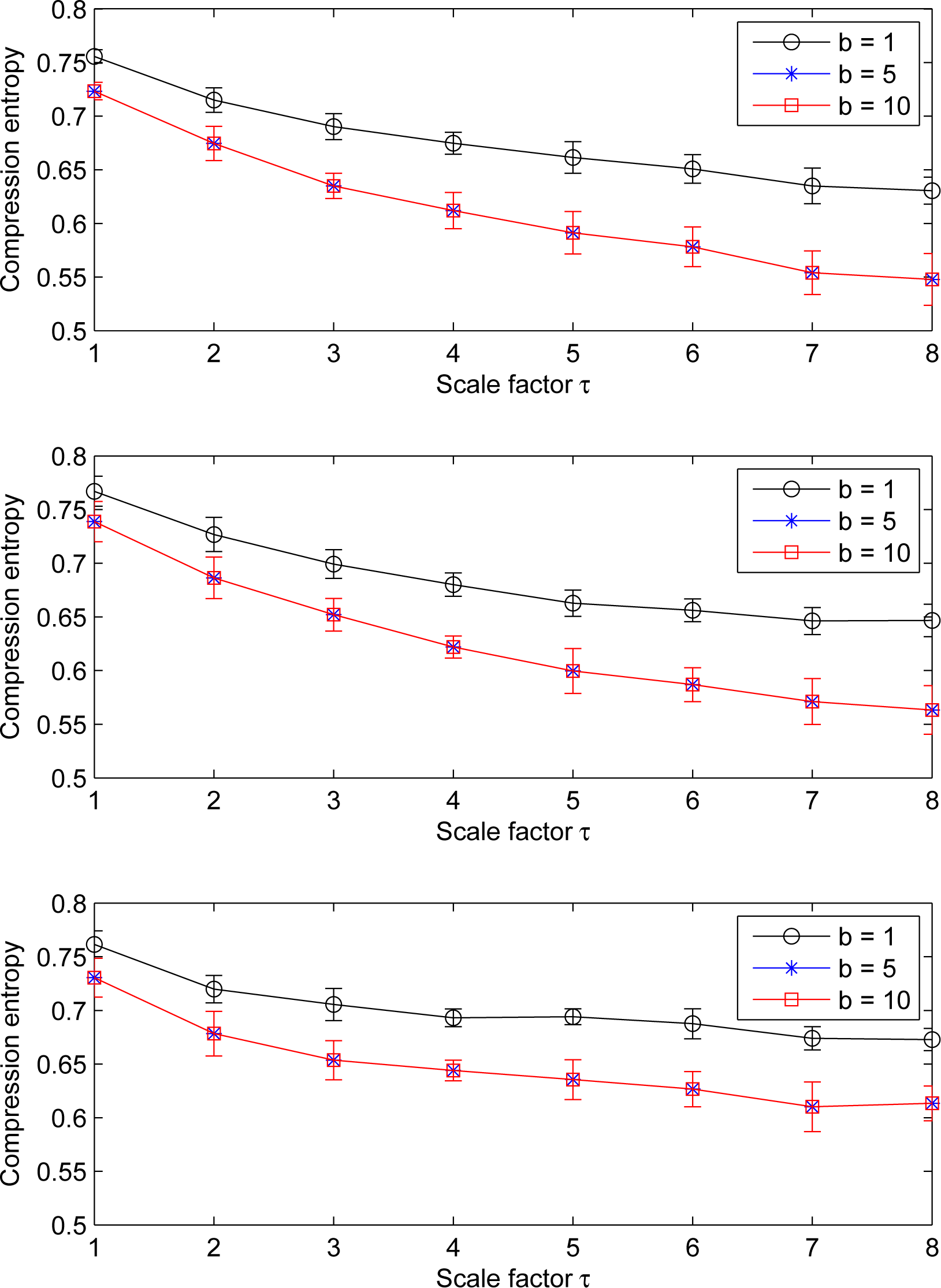
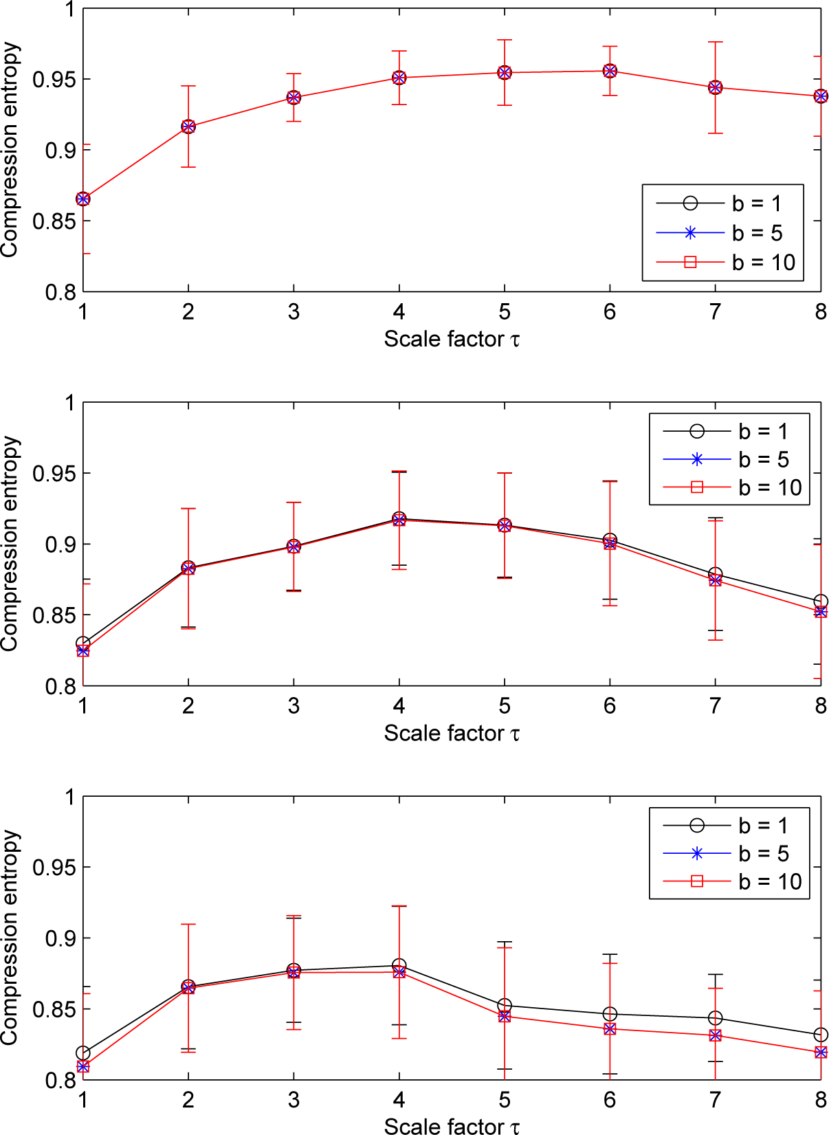
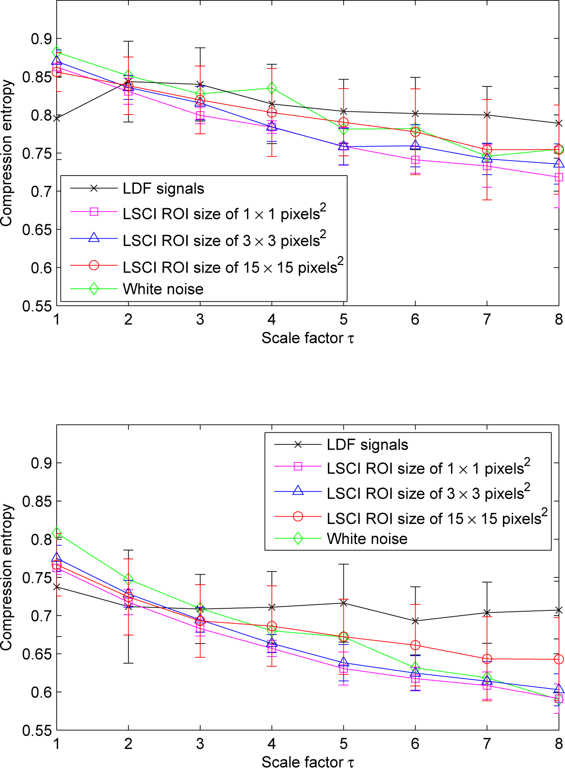
Our results show that, for LSCI data, the pattern of the compression entropy shows a global decreasing trend with scales, whatever the ROI size chosen and whatever the window size w or the lookahead buffer size b (see Figures 4 and 5). However, this decrease is less pronounced with the largest ROI size considered (15 × 15 pixels2); see Figure 6.
Moreover, we note that, for a given sliding window size w larger than one and for all of the ROI sizes, the compression entropy values are higher for a lookahead buffer size b = 1 than for the other buffer sizes (see Figures 4 and 5).
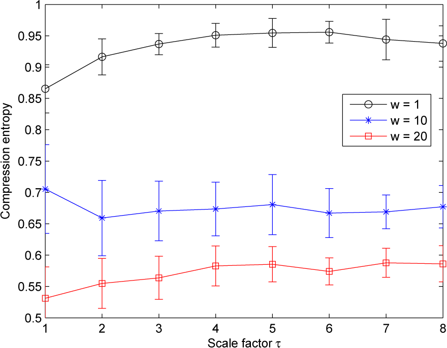
Furthermore, for a given lookahead buffer size b and a given scale factor τ, the compression entropy values decrease when the window size w increases. This is true for the three ROI sizes analyzed (see Figure 7). All of the compression entropy values are between 0.45 and 0.96.
We also note that, for scale factors larger than three, the highest ROI size gives the highest compression entropy values and, therefore, the lowest decreasing trend (see Figure 6).
3.2. Results on LDF Signals
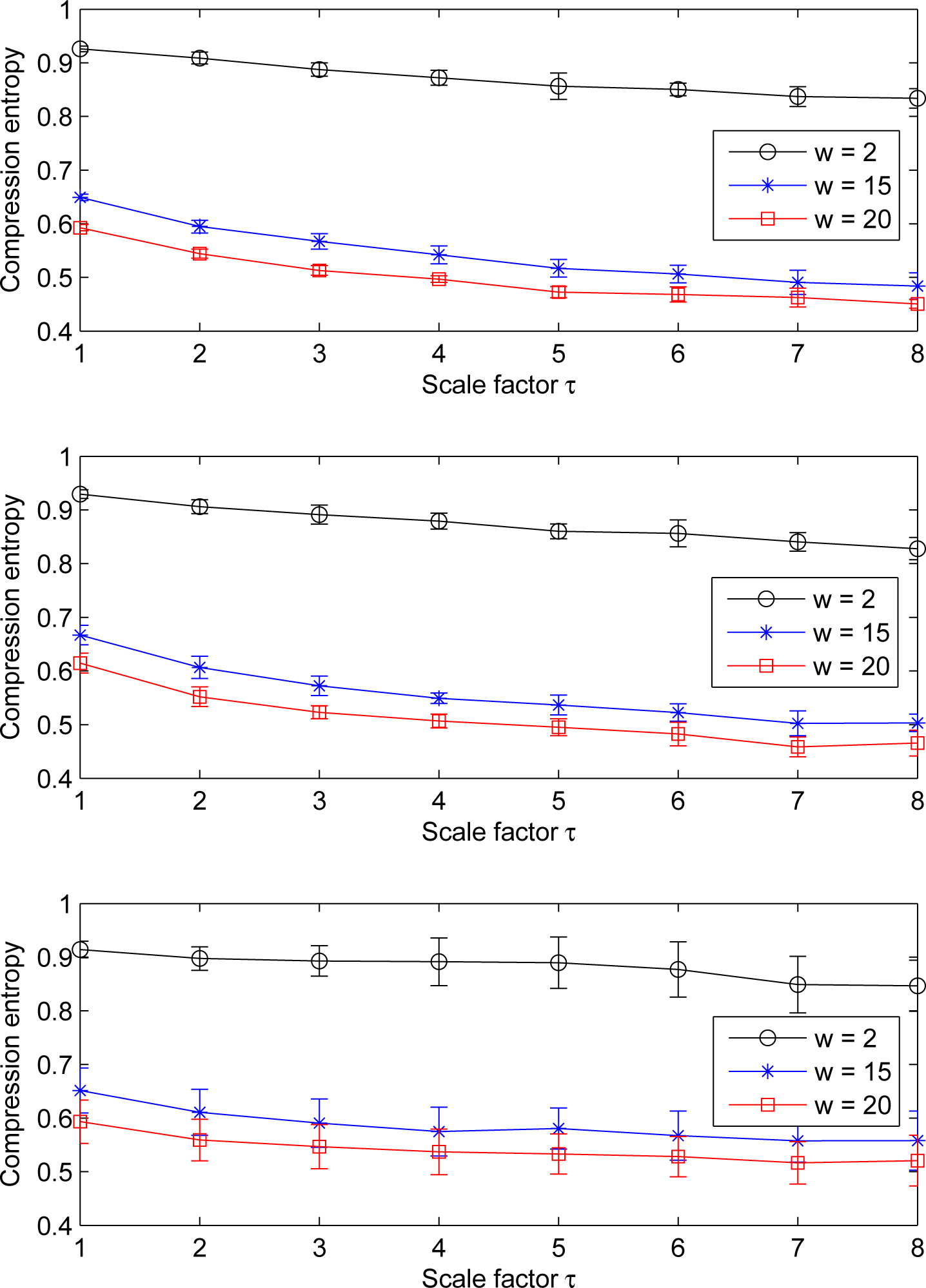
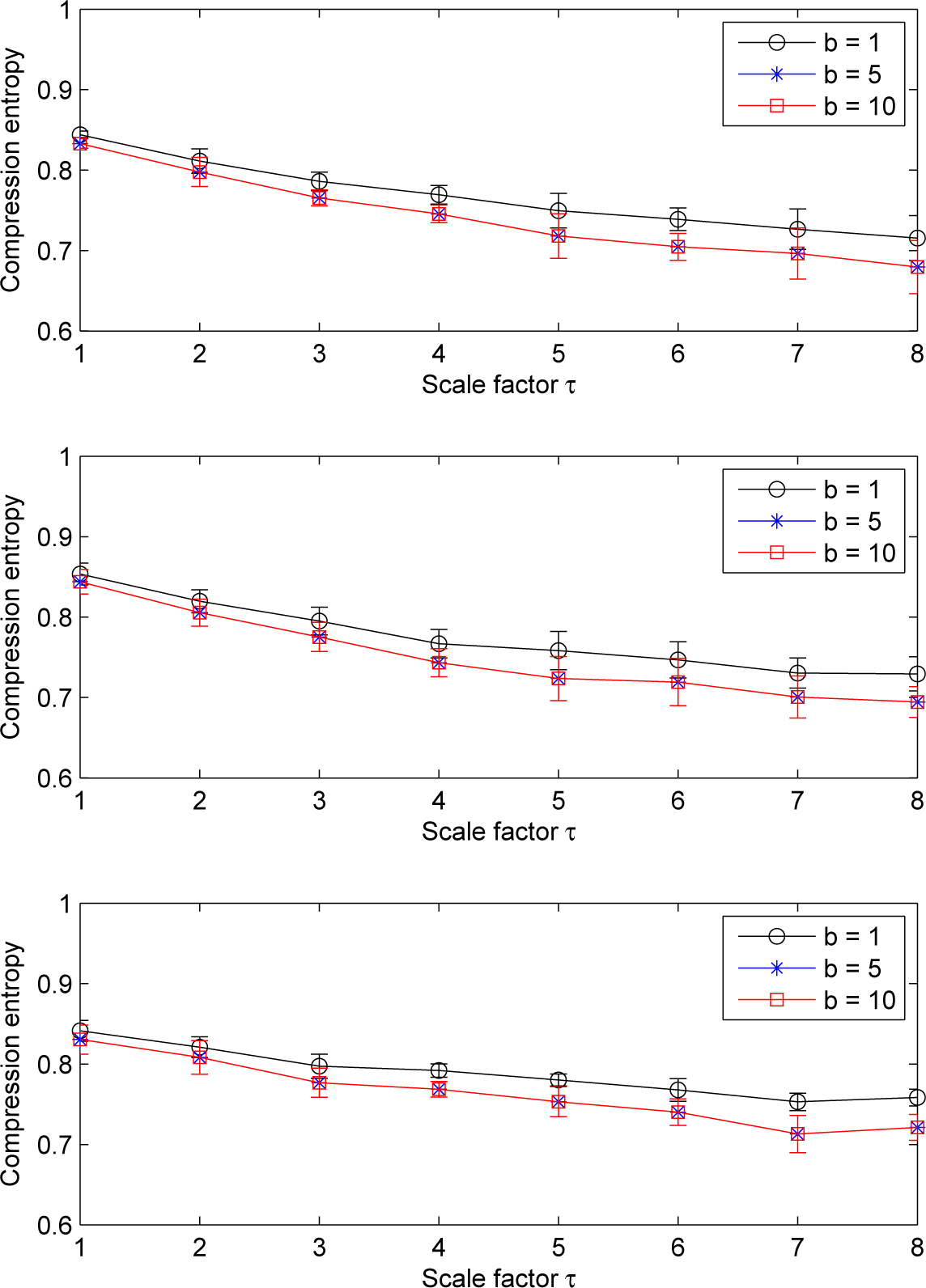
For LDF signals, our results show that the pattern of the multiscale compression entropy when the window size w changes. For a window size w between one and four, we observe an of the compression entropy from scale factor τ = 1 to a distinctive scale factor τ (the value of τ on the window size w) and then a decrease till scale factor τ = 8 (see Figure 8). This non-monotonic pattern is the same for all of the lookahead buffer sizes b analyzed (1 ≤ b ≤ 10): the curves are close whatever the value of the lookahead buffer size (see Figure 8). For sliding windows larger than four, the increasing trend is less pronounced (see Figure 9).
Moreover, we observe that the compression entropy values are lower than one for all of the scales analyzed and for all of the window sizes w and lookahead buffer sizes b studied. For a given lookahead buffer size b and a given scale factor τ, the compression entropy decreases when the sliding window size w increases; see Figure 10.
We also note that, for scale factors larger than three, compression entropy values of LDF signals become larger than the ones of LSCI time series, whatever the ROI sizes and the sliding window size w (see Figure 11).
4. Discussion
The measure of entropy used in the present study describes the information contained in the time series as a ratio of compressed time series length to original time series length. Our results show that compression entropy values for LSCI and LDF time series are less than one for all of the scales analyzed, suggesting that, for all of the scales, there are repetitive structures within the data fluctuations.
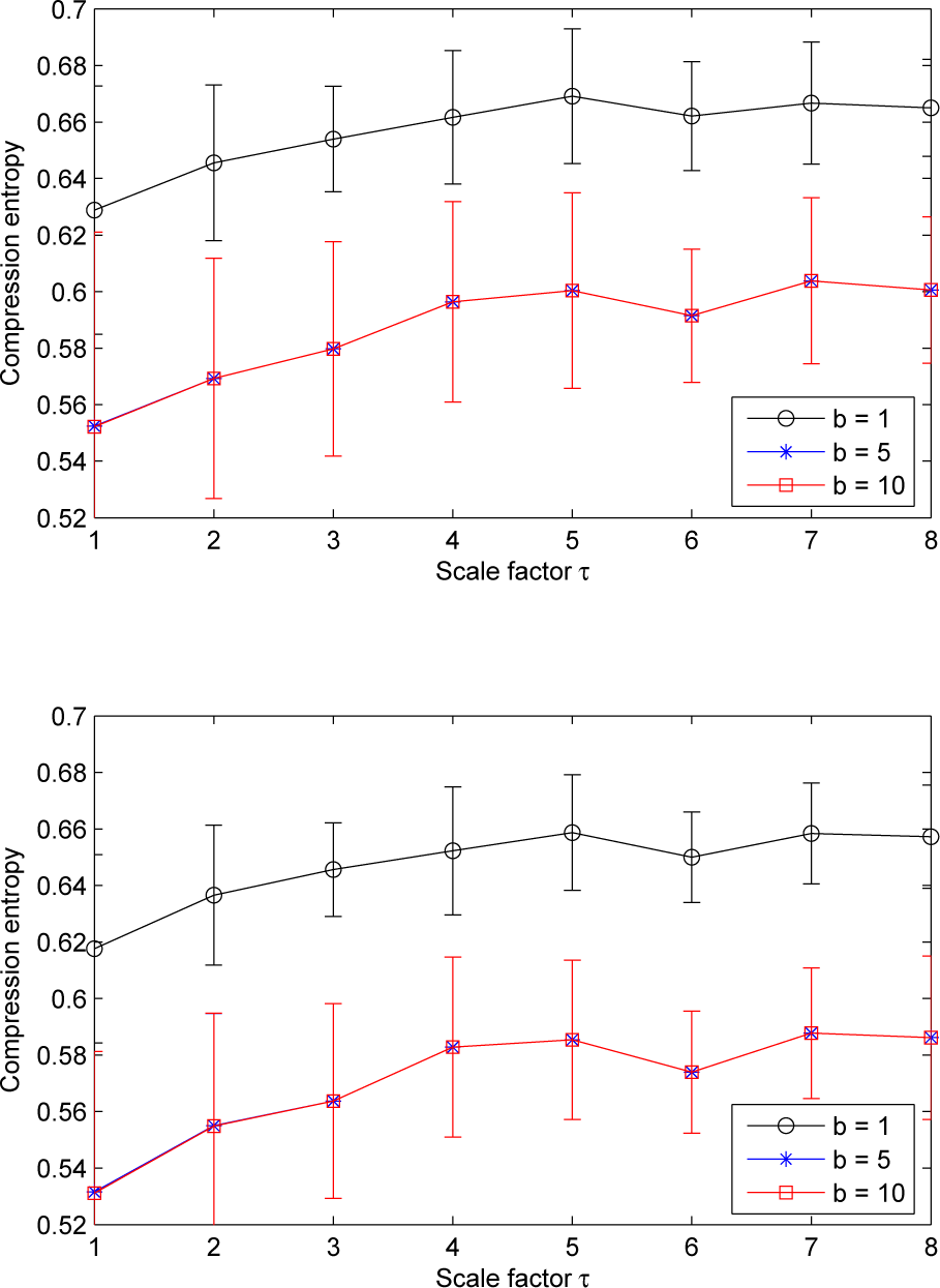
We also report that, for LSCI time series, the pattern of the multiscale compression entropy shows a global decreasing trend with scales, especially for the smallest ROI sizes chosen on LSCI data (1 × 1 pixels2 and 3 × 3 pixels2) and whatever the window size w or the lookahead buffer size b. This decrease is similar to the one observed for Gaussian white noise (see Figure 11). Thus, for white noise, as the length of the window used for coarse-graining increases, the average value inside each window converges to a fixed value, because no new structures exist on larger scales (when the time scales increase, no new structures are revealed). Therefore, the standard deviation monotonically decreases with the scale factor, and the same is found for compression entropy. The global decreasing trend observed for LSCI time series computed from the smallest ROI sizes are in accordance with other works, where it has been reported that LSCI single pixels (or small ROI sizes) in time have statistical properties similar to those of white noise [31,32]. It has also been reported that, for larger ROI sizes on LSCI data, the signal-to-noise ratio increases and the behavior asymptotically approaches the one of LDF [31,32]. Our findings are therefore consistent with these previous results.
Moreover, for LSCI and LDF time series, we observe that the compression entropy values decrease when the window size w increases. Improved compressibility for larger windows might be due to the fact that matching patterns are more likely. This could be due to physiological activities. Other works are needed to better understand these variations. It should also be noted that larger values for the window size w increase the temporal duration of the dynamics that are considered. We also observe that, for scale factors larger than three, compression entropy values of LDF signals become larger than the ones of LSCI time series, but are closer to the ones of LSCI time series computed with an ROI size of 15×15 pixels2 than to the ones computed with smaller ROI sizes. This means that, for scale factors larger than three, LDF signals complexity becomes closer to the ones of LSCI time series with the largest ROI size. These results are in accordance with previous works where it has been reported that: (i) there are different dynamical patterns for LSCI and LDF data [26]; (ii) when the ROI size increases in LSCI data and when LSCI pixel values are averaged in ROI and followed with time, the patterns of the resulting time series approach the patterns of LDF signals [26,31,32,38].
Several studies have been carried on compression entropy [34,37,39–46]. Through these works, it has been shown that compression entropy is sensitive to vagal heart rate modulation [40]. Moreover, some authors reported different entropy functions of heart rate variability (HRV) before the onset of ventricular tachycardia [34,42] and a decrease of the compression entropy of HRV time series of athletes after a training camp compared to the one computed before the training camp [39]. Furthermore, through compression entropy analyses, some authors have shown a significant reduction in the complexity of heart rate modulation in acute, untreated patients suffering from schizophrenia compared to control subjects [41,46]. Studies on HRV from patients with chronic heart failure and type 1 diabetes mellitus have also been conducted [43,44]. Thus, it has been shown that compression entropy is significantly lower in high risk heart failure subjects than in low risk heart failure subjects and that compression entropy is significantly reduced in patients with type 1 diabetes mellitus compared to healthy controls [44]. The influence of negative mood on heart rate compression entropy in healthy subjects has also been investigated [45].
However, very few studies used compression entropy on multiple time scales [37]. Computation of compression entropy on multiple time scales was applied on RR interval time series recorded in young and aged subjects [37]. The authors reported significantly different entropy characteristics over multiple time scales for aged than for younger subjects [37]. Reduced heart rate variability in elderly subjects is well known and has been hypothesized to be caused by reduced vagal heart rate modulations [47]. However, from the best of our knowledge, compression entropy on single or multiple time scales has never been studied nor on LSCI data nor on LDF time series. Our work shows that LSCI and LDF signals contain repetitive structures within their fluctuations. Moreover, the compression entropy decreases when the window size w increases. Further work is needed in order to analyze the role played by the physiological activities in this decrease. Compression entropy may also depend on data frequency acquisition, because the latter may modify the alphabet in which the time series take their sample values. Our data were sampled to 18 Hz, but further investigations are needed to analyze how compression entropy values may change with the sampling rate. Furthermore, future works have to be conducted to compare multiscale compression entropy values in healthy and pathologic subjects.
In our work, the multiscale assessment has been performed on eight scales postulating that at least 200 samples are required for reliable entropy estimation. In their initial algorithm dealing with multiscale entropy (algorithm based on sample entropy), Costa et al. proposed that the shortest coarse-grained time series from the cardiovascular system contained 1,000 samples or even more [36,48]. The latter authors mentioned that the minimum number of data points required applying the multiscale entropy method depends on the level of accepted uncertainty. For the multiscale compression entropy algorithm used in our study, further work is needed to determine the optimal length of the time series at the maximum scale.
LSCI and LDF techniques are, by definition, very sensitive to movements. Therefore, long recordings (several hours or even minutes) cannot be obtained without having numerous movement artifacts. As a consequence, the time scales studied with multiscale compression entropy cannot reach the ones where physiological activities have been traditionally studied.
5. Conclusions
Our findings show that LSCI and LDF signals present compression entropy values lower than one for all of the scales analyzed. This suggests that, for all scales, there are repetitive structures within the data fluctuations. Moreover, for scale factors larger than three, compression entropy values of LDF signals become larger than the ones of LSCI time series, but are closer to the ones of LSCI time series computed with an ROI size of 15 × 15 pixels2 than to the ones computed with smaller ROI sizes. For scale factors larger than three, LDF complexity may therefore become different from the one of LSCI time series, but the larger the ROI size on LSCI data, the closer the complexity of LSCI time series to the one of LDF signals. Finally, LDF signals at larger scales seem to have structures that are different from those of a Gaussian white noise process. This is not observed for LSCI time series when small ROI sizes are taken into account.
Author Contributions
Anne Humeau-Heurtier processed, analyzed and interpreted the data. She also drafted the article. Mathias Baumert performed the coding of the compression entropy and did the statistical tests. He also interpreted the data and drafted the article. Guillaume Mahé and Pierre Abraham were responsible for data collection. They also performed a critical revision of the manuscript. All authors have read and approved the final manuscript.
Conflicts of Interest
The authors declare no conflict of interest.
References
- Maric-Bilkan, C.; Flynn, E.R.; Chade, A.R. Microvascular disease precedes the decline in renal function in the streptozotocin-induced diabetic rat. Am. J. Physiol. Renal. Physiol. 2012, 302, F308–F315. [Google Scholar]
- Jung, F.; Pindur, G.; Ohlmann, P.; Spitzer, G.; Sternitzky, R.; Franke, R.P.; Leithäuser, B.; Wolf, S.; Park, J.W. Microcirculation in hypertensive patients. Biorheology 2013, 50, 241–255. [Google Scholar]
- Stirban, A. Microvascular dysfunction in the context of diabetic neuropathy. Curr. Diab. Rep. 2014, 14, 541. [Google Scholar]
- Jan, Y.K.; Brienza, D.M.; Geyer, M.J. Analysis of week-to-week variability in skin blood flow measurements using wavelet transforms. Clin. Physiol. Funct. Imaging 2005, 25, 253–262. [Google Scholar]
- Allen, J.; Howell, K. Microvascular imaging: Techniques and opportunities for clinical physiological measurements. Physiol. Meas. 2014, 35, R91–R141. [Google Scholar]
- Stern, M.D. In vivo evaluation of microcirculation by coherent light scattering. Nature 1975, 254, 56–58. [Google Scholar]
- Briers, D.; Duncan, D.D.; Hirst, E.; Kirkpatrick, S.J.; Larsson, M.; Steenbergen, W.; Stromberg, T.; Thompson, O.B. Laser speckle contrast imaging: Theoretical and practical limitations. J. Biomed. Opt. 2013, 18, 066018. [Google Scholar]
- Humeau-Heurtier, A.; Guerreschi, E.; Abraham, P.; Mahé, G. Relevance of laser Doppler and laser speckle techniques for assessing vascular function: State of the art and future trends. IEEE Trans. Biomed. Eng. 2013, 60, 659–666. [Google Scholar]
- Bonner, R.; Nossal, R. Model for laser Doppler measurements of blood flow in tissue. Appl. Opt. 1981, 20, 2097–2107. [Google Scholar]
- Essex, T.J.; Byrne, P.O. A laser Doppler scanner for imaging blood flow in skin. J. Biomed. Eng. 1991, 13, 189–194. [Google Scholar]
- Wardell, K.; Jakobsson, A.; Nilsson, G.E. Laser Doppler perfusion imaging by dynamic light scattering. IEEE Trans. Biomed. Eng. 1993, 40, 309–316. [Google Scholar]
- Leutenegger, M.; Martin-Williams, E.; Harbi, P.; Thacher, T.; Raffoul, W.; André, M.; Lopez, A.; Lasser, P.; Lasser, T. Real-time full field laser Doppler imaging. Biomed. Opt. Express 2011, 2, 1470–1477. [Google Scholar]
- Fercher, A.F.; Briers, J.D. Flow visualization by means of single-exposure speckle photography. Opt. Comm. 1981, 37, 326–330. [Google Scholar]
- Briers, J.D.; Webster, S. Laser speckle contrast analysis (LASCA): A nonscanning, full-field technique for monitoring capillary blood flow. J. Biomed. Opt. 1996, 1, 174–179. [Google Scholar]
- Boas, D.A.; Dunn, A.K. Laser speckle contrast imaging in biomedical optics. J. Biomed. Opt. 2010, 15, 011109. [Google Scholar]
- Richards, L.M.; Kazmi, S.M.; Davis, J.L.; Olin, K.E.; Dunn, A.K. Low-cost laser speckle contrast imaging of blood flow using a webcam. Biomed. Opt. Express 2013, 4, 2269–2283. [Google Scholar]
- Humeau, A.; Saumet, J.L.; L’Huillier, J.P. Use of wavelets to accurately determine parameters of laser Doppler reactive hyperemia. Microvasc. Res. 2000, 60, 141–148. [Google Scholar]
- Stefanovska, A.; Bracic, M.; Kvernmo, H.D. Wavelet analysis of oscillations in the peripheral blood circulation measured by laser Doppler technique. IEEE Trans. Biomed. Eng. 1999, 46, 1230–1239. [Google Scholar]
- Humeau, A.; Chapeau-Blondeau, F.; Rousseau, D.; Rousseau, P.; Trzepizur, W.; Abraham, P. Multifractality, sample entropy, and wavelet analyses for age-related changes in the peripheral cardiovascular system: Preliminary results. Med. Phys. 2008, 35, 717–723. [Google Scholar]
- Figueiras, E.; Roustit, M.; Semedo, S.; Ferreira, L.F.; Crascowski, J.L.; Humeau, A. Sample entropy of laser Doppler flowmetry signals increases in patients with systemic sclerosis. Microvasc. Res. 2011, 82, 152–155. [Google Scholar]
- Humeau, A.; Mahé, G.; Chapeau-Blondeau, F.; Rousseau, D.; Abraham, P. Multiscale analysis of microvascular blood flow: A multiscale entropy study of laser Doppler flowmetry time series. IEEE Trans. Biomed. Eng. 2011, 58, 2970–2973. [Google Scholar]
- Jan, Y.K.; Lee, B.; Liao, F.; Foreman, R.D. Local cooling reduces skin ischemia under surface pressure in rats: An assessment by wavelet analysis of laser Doppler blood flow oscillations. Physiol. Meas. 2012, 33, 1733–1745. [Google Scholar]
- Humeau-Heurtier, A.; Buard, B.; Mahe, G.; Abraham, P. Laser speckle contrast imaging of the skin: Interest in processing the perfusion data. Med. Biol. Eng. Comput. 2012, 50, 103–105. [Google Scholar]
- Millet, C.; Roustit, M.; Blaise, S.; Cracowski, J.L. Comparison between laser speckle contrast imaging and laser Doppler imaging to assess skin blood flow in humans. Microvasc. Res. 2011, 82, 147–151. [Google Scholar]
- Binzoni, T.; Humeau-Heurtier, A.; Abraham, P.; Mahe, G. Blood perfusion values of laser speckle contrast imaging and laser Doppler flowmetry: Is a direct comparison possible? IEEE Trans. Biomed. Eng. 2013, 60, 1259–1265. [Google Scholar]
- Humeau-Heurtier, A.; Abraham, P.; Mahe, G. Linguistic analysis of laser speckle contrast images recorded at rest and during biological zero: Comparison with laser Doppler flowmetry data. IEEE Trans. Med. Imaging 2013, 32, 2311–2321. [Google Scholar]
- Puissant, C.; Abraham, P.; Durand, S.; Humeau-Heurtier, A.; Faure, S.; Lefthériotis, G.; Rousseau, P.; Mahé, G. Reproducibility of non-invasive assessment of skin endothelial function using laser Doppler flowmetry and laser speckle contrast imaging. PLoS One 2013, 8, e61320. [Google Scholar]
- O’Doherty, J.; McNamara, P.; Clancy, N.T.; Enfield, J.G.; Leahy, M.J. Comparison of instruments for investigation of microcirculatory blood flow and red blood cell concentration. J. Biomed. Opt. 2009, 14, 034025. [Google Scholar]
- Humeau-Heurtier, A.; Mahe, G.; Durand, S.; Abraham, P. Skin perfusion evaluation between laser speckle contrast imaging and laser Doppler flowmetry. Opt. Commun. 2013, 291, 482–487. [Google Scholar]
- Mahe, G.; Haj-Yassin, F.; Rousseau, P.; Humeau, A.; Durand, S.; Leftheriotis, G.; Abraham, P. Distance between laser head and skin does not influence skin blood flow values recorded by laser speckle imaging. Microvasc. Res. 2011, 82, 439–442. [Google Scholar]
- Humeau-Heurtier, A.; Mahe, G.; Durand, S.; Henrion, D.; Abraham, P. Laser speckle contrast imaging: Multifractal analysis of data recorded in healthy subjects. Med. Phys. 2012, 39, 5849–5856. [Google Scholar]
- Humeau-Heurtier, A.; Mahé, G.; Durand, S.; Abraham, P. Multiscale entropy study of medical laser speckle contrast images. IEEE Trans. Biomed. Eng. 2013, 60, 872–879. [Google Scholar]
- Li, M.; Vitányi, P. An introduction to Kolmogorov complexity and its applications; Springer Verlag: New-York, NY, USA, 1997. [Google Scholar]
- Baumert, M.; Baier, V.; Haueisen, J.; Wessel, N.; Meyerfeldt, U.; Schirdewan, A.; Voss, A. Forecasting of life threatening arrhythmias using the compression entropy of heart rate. Methods Inf. Med. 2004, 43, 202–206. [Google Scholar]
- Ziv, J.; Lempel, A. A universal algorithm for sequential data compression. IEEE Trans. Inf. Theory 1977, 23, 337–343. [Google Scholar]
- Costa, M.; Goldberger, A.L.; Peng, C.K. Multiscale entropy analysis of complex physiologic time series. Phys. Rev. Lett. 2002, 89, 068102. [Google Scholar]
- Baumert, M.; Voss, A.; Javorka, M. Compression based entropy estimation of heart rate variability on multiple time scales, Proceedings of the 35th International Conference of the IEEE EMBS, Osaka, Japan, 3–7 July 2013; pp. 5037–5040.
- Bricq, S.; Mahé, G.; Rousseau, D.; Humeau-Heurtier, A.; Chapeau-Blondeau, F.; Varela, J.R.; Abraham, P. Assessing spatial resolution versus sensitivity from laser speckle contrast imaging: Application to frequency analysis. Med. Biol. Eng. Comput. 2012, 50, 1017–1023. [Google Scholar]
- Baumert, M.; Baier, V.; Voss, A. Estimating the complexity of heart rate fluctuations—An approach based on compression entropy. Fluct. Noise Lett. 2005, 5, L557–L563. [Google Scholar]
- Baumert, M.; Nalivaiko, E.; Abbott, D. Effects of vagal blockade on the complexity of heart rate variability in rats. IFMBE Proc. 2007, 16, 26–29. [Google Scholar]
- Bär, K.J.; Boettger, M.K.; Koschke, M.; Schulz, S.; Chokka, P.; Yeragani, V.K.; Voss, A. Non-linear complexity measures of heart rate variability in acute schizophrenia. Clin. Neurophysiol. 2007, 118, 2009–2015. [Google Scholar]
- Baumert, M.; Wessel, N.; Schirdewan, A.; Voss, A.; Abbott, D. Forecasting of ventricular tachycardia using scaling characteristics and entropy of heart rate time series. IFMBE Proc. 2007, 14, 1001–1004. [Google Scholar]
- Voss, A.; Schroeder, R.; Vallverdu, M.; Cygankiewicz, I.; Vazquez, R.; Bayes de Luna, A.; Caminal, P. Linear and nonlinear heart rate variability risk stratification in heart failure patients. Comput. Cardiol. 2008, 35, 557–560. [Google Scholar]
- Javorka, M.; Trunkvalterova, Z.; Tonhajzerova, I.; Javorkova, J.; Javorka, K.; Baumert, M. Short-term heart rate complexity is reduced in patients with type 1 diabetes mellitus. Clin. Neurophysiol. 2008, 119, 1071–1081. [Google Scholar]
- Köbele, R.; Koschke, M.; Schulz, S.; Wagner, G.; Yeragani, S.; Ramachandraiah, C.T.; Voss, A.; Yeragani, V.K.; Bär, K.J. The influence of negative mood on heart rate complexity measures and baroreflex sensitivity in healthy subjects. Indian J. Psychiatry 2010, 52, 42–47. [Google Scholar]
- Rachow, T.; Berger, S.; Boettger, M.K.; Schulz, S.; Guinjoan, S.; Yeragani, V.K.; Voss, A.; Bär, K.J. Nonlinear relationship between electrodermal activity and heart rate variability in patients with acute schizophrenia. Psychophysiology 2011, 48, 1323–1332. [Google Scholar]
- Voss, A.; Heitmann, A.; Schroeder, R.; Peters, A.; Perz, S. Short-term heart rate variability—Age dependence in healthy subjects. Physiol. Meas. 2012, 33, 1289–1311. [Google Scholar]
- Costa, M.; Goldberger, A.L.; Peng, C.K. Multiscale entropy analysis of biological signals. Phys. Rev. E 2005, 71, 021906. [Google Scholar]


© 2014 by the authors; licensee MDPI, Basel, Switzerland This article is an open access article distributed under the terms and conditions of the Creative Commons Attribution license (http://creativecommons.org/licenses/by/4.0/).
Share and Cite
Humeau-Heurtier, A.; Baumert, M.; Mahé, G.; Abraham, P. Multiscale Compression Entropy of Microvascular Blood FlowSignals: Comparison of Results from Laser Speckle Contrastand Laser Doppler Flowmetry Data in Healthy Subjects. Entropy 2014, 16, 5777-5795. https://doi.org/10.3390/e16115777
Humeau-Heurtier A, Baumert M, Mahé G, Abraham P. Multiscale Compression Entropy of Microvascular Blood FlowSignals: Comparison of Results from Laser Speckle Contrastand Laser Doppler Flowmetry Data in Healthy Subjects. Entropy. 2014; 16(11):5777-5795. https://doi.org/10.3390/e16115777
Chicago/Turabian StyleHumeau-Heurtier, Anne, Mathias Baumert, Guillaume Mahé, and Pierre Abraham. 2014. "Multiscale Compression Entropy of Microvascular Blood FlowSignals: Comparison of Results from Laser Speckle Contrastand Laser Doppler Flowmetry Data in Healthy Subjects" Entropy 16, no. 11: 5777-5795. https://doi.org/10.3390/e16115777
APA StyleHumeau-Heurtier, A., Baumert, M., Mahé, G., & Abraham, P. (2014). Multiscale Compression Entropy of Microvascular Blood FlowSignals: Comparison of Results from Laser Speckle Contrastand Laser Doppler Flowmetry Data in Healthy Subjects. Entropy, 16(11), 5777-5795. https://doi.org/10.3390/e16115777