Entropy and Equilibria in Competitive Systems

Abstract
: This paper investigates the applicability of thermodynamic concepts and principles to competitive systems. We show that Tsallis entropies are suitable for the characterisation of systems with transitive competition when mutations deviate from Gibbs mutations. Different types of equilibria in competitive systems are considered and analysed. As competition rules become more and more intransitive, thermodynamic analogies are eroded, and the behaviour of the system can become complex. This work analyses the phenomenon of punctuated evolution in the context of the competitive risk/benefit dilemma.1. Introduction
The question of whether systems involving competition can be characterised by quantities resembling conventional thermodynamic parameters does not have a simple unambiguous answer. This problem was investigated in [1], and it was found that such a characterisation is possible under conditions of transitive competition, but as the system becomes more and more intransitive, the thermodynamic analogy weakens. The similarity with conventional thermodynamic principles is strongest when mutations present in the system belong to the class of Gibbs mutations. While deploying the conventional logarithmic definition of entropy, the analysis of [1] misses an important point: when mutations deviate from the Gibbs mutations, the family of Tsallis entropies [2] represents a very convenient choice of entropy to treat these cases. This omission is rectified in the present work. We also note that Tsallis entropy has been recently used in the modelling of biological replications [3].
Thermodynamics is strongly linked to the concept of equilibrium. Competitive systems allow the introduction of different types of equilibrium, possessing different degrees of similarity with the concept of equilibrium in conventional thermodynamics. The current work discusses possible cases of competitive equilibria and performs a detailed analysis based on the Tsallis entropy of the equilibrium through a point of contact, which is more similar to conventional thermodynamics than the other cases.
From the thermodynamic perspective, the present work is only an example of using Tsallis entropy. We do not attempt to draw any general thermodynamic conclusions, and the use of non-extensive entropy in other applications may well be different from our treatment of equilibria in completive systems. The problem of general consistency between physical equilibrium conditions and definitions of non-extensive entropies has been analysed by Abe [4,5]. Non-extensive statistical mechanics has been reviewed by Tsallis [2], while non-extensive entropies associated with this mechanics are discussed in [2–7] and many other publications.
The last section deals with intransitive cases when the thermodynamic analogy weakens, and the possibility of using entropy as a quantity that always tends to increase in time or remain constant is not assured. This section analyses the risk/benefit dilemma represented by a competitive system, whose evolution can be transitive or intransitive, depending on the choice of the system parameters. In the intransitive case, the evolution of the system appears to be punctuated by sudden collapses and becomes cyclic. This punctuated evolution is similar to the concept of punctuated equilibrium in evolutionary biology [8], although in the context of thermodynamics, the latter term might be misleading, as the system is not in equilibrium and keeps evolving between the punctuations.
2. Competitive Systems
Competitive systems involve the process of competition in its most generic form. The elements of competitive systems compete with each other according to preset rules. The rules define the winners and losers for each competition round based on properties of the elements, denoted here by y. The properties of the losers are lost while the winners utilise the resource vacated by the losers and duplicate their properties. The process of duplication is not perfect and involves random mutations, which are mostly detrimental for the competitiveness of the elements. The expression, A ≺ B, (or, equivalently, yA ≺ yB) indicates that element B with properties yB is the winner in competition with element A with properties yA. If two elements have equivalent strength yA ≃ yB, the winner is to be determined at random. In computer simulations, the elements are also called Pope particles, and the exchange of properties is called mixing by analogy, with the conventions adopted in particle simulations of reacting flows. Two forms of mixing—conservative and competitive—can be distinguished. The former is predominantly used in the flow simulations, while the latter is associated with competitive systems. The rest of this section introduces the basic terms used in the characterisation of competitive systems; further details can be found in [1,9].
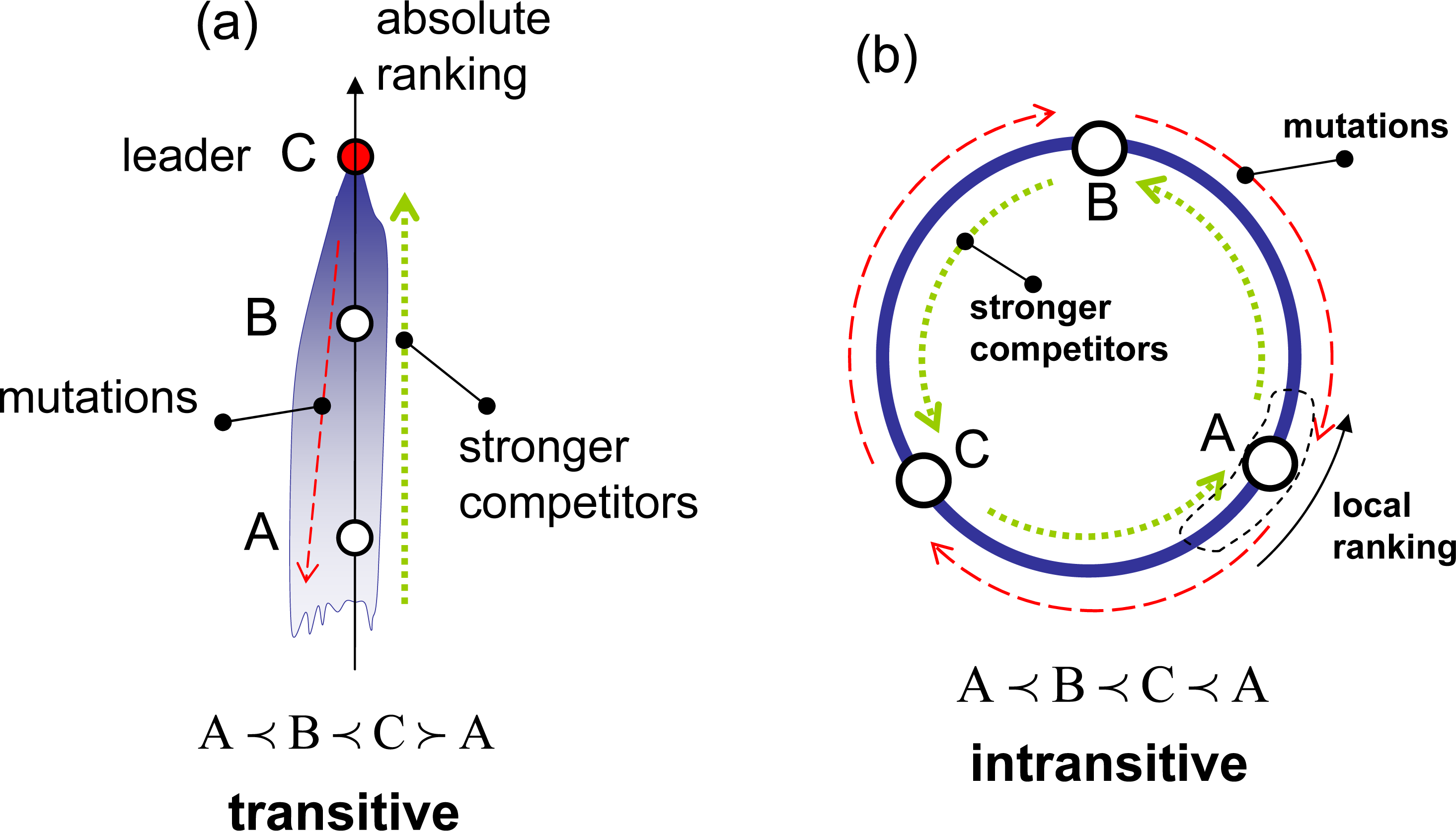
The competition rules are divided into two major categories: transitive and intransitive. In transitive competitions, the superiority of B over A and C over B inevitably demands the superiority of C over A, that is:
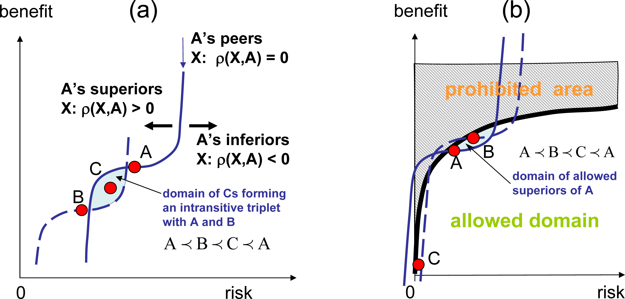
As illustrated in Figure 1a, transitive competitions enable the introduction of an absolute ranking, r(y), which is a numerical function that determines superior (stronger) and inferior (weaker) elements:
The competition rules, however, are not necessarily transitive, and the competition is deemed intransitive when at least one intransitive triplet:
The distributions of elements in the property space is characterised by the particle distribution function φ(y) = nf(y), where n is the total number of particles and f(y), which can be interpreted as the probability distribution function (pdf), satisfies the normalisation condition:
Examples of systems using competitive mixing can be found in [1,9–11]
3. Competition and q-Exponential Distributions
We consider transitive competition with elements possessing a scalar property y, which is selected to be aligned with ranking (that is r(y) is a monotonically increasing function, and the absolute ranking is effectively specified by y). Hence, for any two elements, A and B:
The Gibbs mutations [1] correspond to q = 1, implying that the distribution, fm(y), is based, in this case, on the conventional exponent:
In this work, we are interested in the case when the pdf, f, can be approximated by the q-exponential distribution:
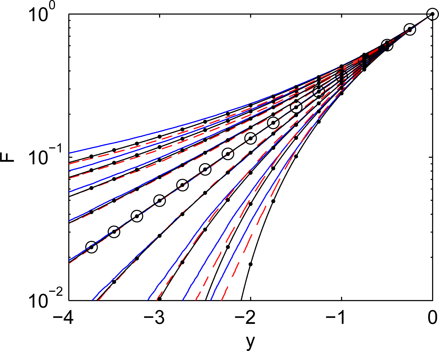
Figure 2 illustrates that, as expected, the cdf of simulated distributions are very close to the corresponding q-exponents when q is close to unity. The q-exponential functions can also serve as very good approximations for distribution in competitive systems for a wide range of q. Consider the q-exponential distribution of mutations:
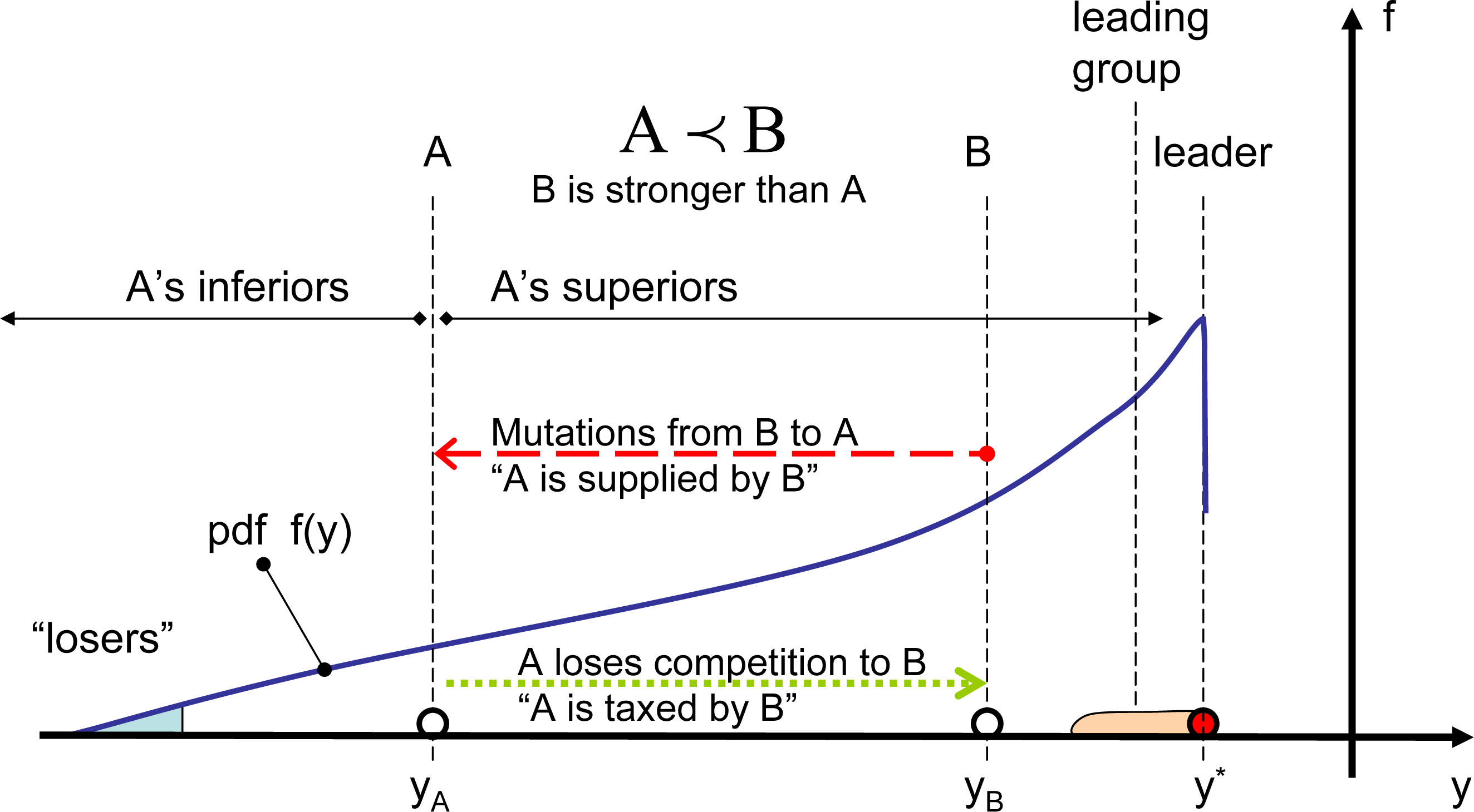
The cdf shapes presented in Figure 2 indicate that, although q-exponential distributions are not necessarily exact for competitive systems, they are reasonably accurate and correspond very well to the physical nature of the problem when mutations deviate from Gibbs mutations. In the competitive system illustrated in Figure 3, every location is taxed, due to competition with superior elements, and, at the same time, is supplied by mutations originating from superior elements. For Gibbs mutations, the competitive system schematically depicted in Figure 3 is in the state of detailed balance: every location is taxed and supplied at the same rate by any given superior. In simple systems with constant a priori phase space A(y), the Gibbs mutations are distributed exponentially (q = 1). When mutations deviate from Gibbs mutations, the overall rates of taxing and supplying must negate each other under steady conditions, but there is no detailed balance in relations with different groups of superiors. For long-tailed (superexponential) distributions with q > 1, weak particles are supplied more by the leaders and are taxed more by immediate superiors. For short-tailed (superexponential) distributions with q < 1, weak particles are supplied more by the immediate superiors and are taxed more by the leaders.
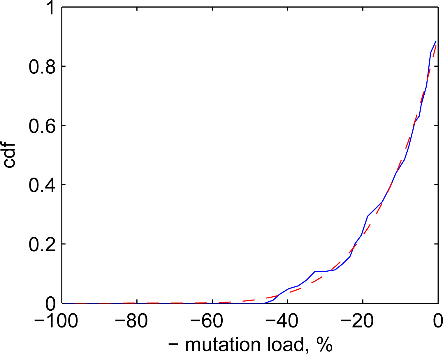
Competitive systems are aimed at studying generic properties of systems with competition and mutations. Although we do not specifically intend to model distributions of biological mutations, these distributions are still of some interest here as real–world examples of complex competitive systems. Ohta [12] considered near-neutral genetic mutations and suggested that these mutations have exponential distributions. Modern works tend to use the Kimura distribution [13], which has a complicated mathematical form, deviates from pure exponents and, theoretically, corresponds to a genetic drift of neutral mutations. It seems that the reported distributions of genetic mutations tend to be slightly subexponential. Figure 4 illustrates that the experimental distribution of mutation A3243G of mitochondrial DNA in humans [13] is well approximated by q-exponential cdf with Q = 0.8. Since these mutations are known to be deleterious [14], they are shown as negative in the figure (in agreement with the notations adopted in the rest of the present work).
4. Tsallis Entropy in Competitive Systems
Free Tsallis entropy in competitive systems is defined by:
♦ The translational case of γ = 1. With Equation (27), Equation (31) takes the form:
that with sy(y) = ky, A = cqq and λ = −ky* results in the pdf and cdf given by:where Q = 1/q and q2 = 2 − q. Since y* is arbitrary in this case, the distribution can be freely shifted along y. The location of y* is determined by Equation (30).♦ The multiplicative case of γ = q. Equations (27) and (31) take the form:
that, with, A = 1 and sy(y) = k (y − y*), results in the pdf:with the arbitrary value of Zq depending on λ. This value can be determined from the normalisation requiring that Zq = k−1/(2 − q). The corresponding cdf, FQ(y, y*), is the same as Equation (33) with the q-parameter given by Q = Zqk = 1/(2 − q).
In the case of physical thermodynamics, Tsallis et al. [6] recommend using γ = q in conjunction with the escort distribution for the energy constraints as the best option. Competitive thermodynamics, as considered here, does not have any energy constraints (assuming that the conservative properties are limited to the number of particles, we do not have any energy defined for the system), and the selection of γ needs to be considered again. The choice of γ for competitive systems is determined by the physics of the problem and can be different for different processes. If infrequently positive mutations are present and the distribution with a fixed number of particles escalates by gradually increasing y* in time, then γ = 1 is preferable. Indeed, while y* increases, the definition of entropy remains exactly the same, and the escalation is seen as a natural process of increasing entropy in the system. If γ = q, the definition of entropy is dependent on the position of the leading particle. The choice of γ = q is more suitable for competitions between subsystems placed at fixed locations, but with the numbers of particles that can be altered due to exchanges. Gibbs mutations correspond to q = 1, and the choices, γ = 1 and γ = q, coincide in this case. In the previous work [1], the Boltzmann–Gibbs entropy was used for non-Gibbs mutations by artificially making the phase volume dependent on the leading particle position A = A(y, y*). Unlike the Tsallis entropy considered in the present work, the old treatment of the problem [1] did not allow for a unified definition of entropy valid for different y* (i.e., the Boltzmann–Gibbs entropy provides a unified, y*-independent definition of competitive entropy only for the Gibbs mutations).
5. Equilibria in Competing Systems
A competitive system can be divided into subsystems, and the question of equilibrium conditions between these subsystems appears. If the system is subdivided into K subsystems I = 1, 2, ..., K and subsystem I has the bI-th fraction of the particles, we may characterise each of these subsystems by its own normalised distribution ϕI(y), as specified by Equations (9) and (10). Assuming that equilibrium or steady-state conditions are achieved within each subsystem, the major equilibrium cases include:
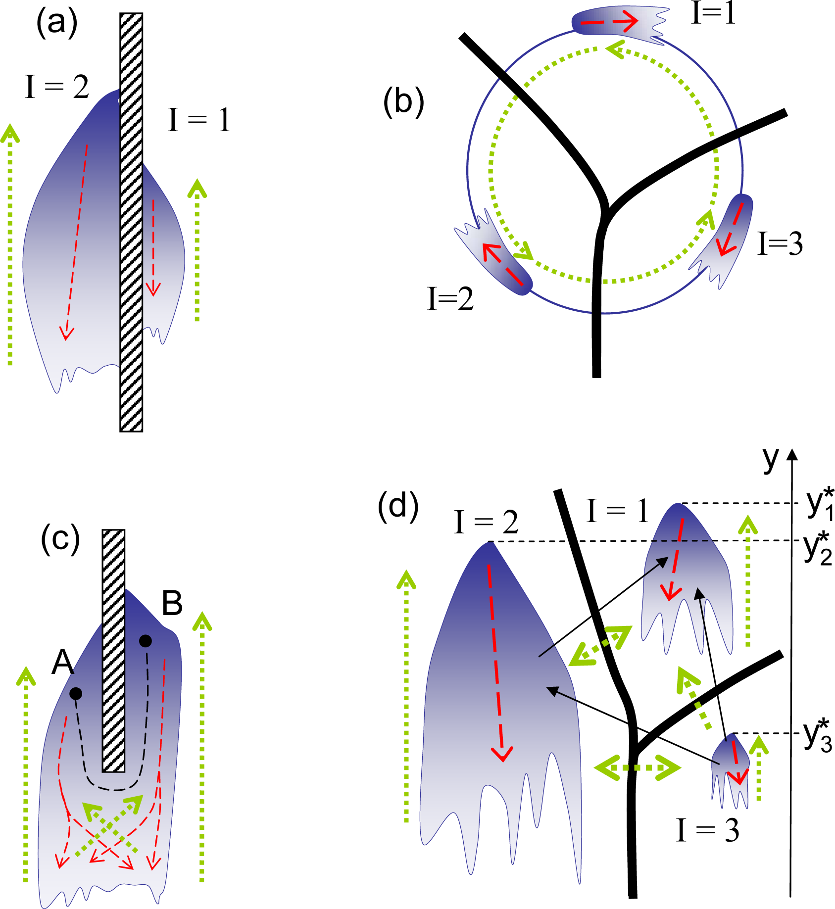
♦ Equilibria in isolated subsystems. Isolated subsystems do not exchange mutations and do not compete against each other. Equilibria are established in isolated subsystems independently of the other subsystems (see Figure 5a)
♦ Competing equilibria. Particles in these subsystems compete against each other, but mutations do not cross the subsystem boundaries as illustrated in Figure 5b. Competing equilibria tend to be less stable than the connected equilibria considered below and, generally, are impossible in transitive competitions. Indeed, if (i.e., the leading element of subsystem I is more competitive than the leading element of subsystem J), cannot lose to any element of subsystem J, while will eventually lose to leading elements of I. There is no equilibrium in the transitive competition depicted in Figure 5d, since the subsystem I = 1 is going to win all particle resources for itself. If , then the two leaders will eventually meet in competition, and due to their equivalent strength, the winner of this round (which ultimately belongs to the winning subsystem) is to be selected at random. Competing equilibria are nevertheless possible in intransitive competitions. This, obviously, requires that:
for all I = 1, ..., K, or, otherwise, nI would grow for RI > 0 and decrease for RI < 0. As discussed in the Appendix of [1], oscillations are to appear in competing equilibria between subsystems 1, …, K, unless:for every I and J, Constraint (37) implies all subsystems should have the same relative strength [ϕI] ≃ [ϕJ], which is a stronger condition than [ϕI] ≃ [f] required by (36). Condition (37) is necessary to avoid oscillations between the subsystems. If present, the oscillations can be stable, neutral or unstable. The example in [1] demonstrates the case when oscillations are unstable. Competing equilibria exist only in competitive systems and, it seems, do not have an analog in conventional thermodynamics.♦ Connected equilibria. In this case, the subsystems I = 1, ..., K are connected by both competition and mutations. For Gibbs mutations (q = 1), the competitive H-theorem applies ensuring the detailed balance of the equilibrium state [1]. This implies that, in equilibrium, the connection between any two elements or groups of elements can be severed without any effect on the state of the system. Severing connection between two elements terminates both competition and mutations between these elements. This is illustrated in Figure 5c, where the direct connection between points A and B is severed, although A and B remain connected through other elements, as shown by the dashed line. The equilibrium conditions are given by the equivalence of all competitive potentials χI = χJ for every I and J, where the formula for competitive potential: [1,9]
is obtained by differentiating entropy with respect to nI. The partition functions, ZI, are evaluated for each subsystem, I, as an integral over the subsystem domain, 𝔇I:Equilibrium in competitive systems with Gibbs mutations resembles most the equilibria of conventional thermodynamics. In the case of general non-positive mutations (i.e., non-Gibbs mutations), the state of the system depends on the type of contact. Here, we distinguish two cases of interest:– Point of contact. Two subsystems, I and J, have a point of contact at y = y° when the elements from the vicinity of y = y° effectively belong to the both subsystems, while the other elements are isolated within their subsystems. Hence, at equilibrium, the density of particles representing competing elements must be the same in both subsystems at the point of contact:
The phase volume associated with the distributions is likely to be the same on both sides AI(y°) = AJ(y°). The existence of a single point of contact (or several points of contact that, as discussed below, do not form a loop, while connecting several subsystems) changes nI, but does not affect the distributions, ϕI(y). More than one point of contact between two systems with non-Gibbs mutations is likely to change not only nI, but, also, the distributions, ϕI(y).– Complete merger. The subsystems are merged into a single system with the overall stationary distribution f = f0(y). Unless mutations are limited to Gibbs mutations, the subsystems are likely to undergo complex adjustments, changing their distributions. If the term equilibrium is used for this steady state, it should be remembered that, generally, there is no detailed balance in the system. The overall stationary distribution is inseparable: f0(y) may change if the contact between any two locations is severed. Note that, although unusual, inseparable systems exist in conventional thermodynamics: objects with negative heat capacity [15] may serve as an example.
Among different types of equilibria in competitive systems, the equilibrium at a point of contact is most suitable for thermodynamic analysis, even when mutations substantially deviate from Gibbs mutations.
6. Entropy for Equilibrium through a Point of Contact
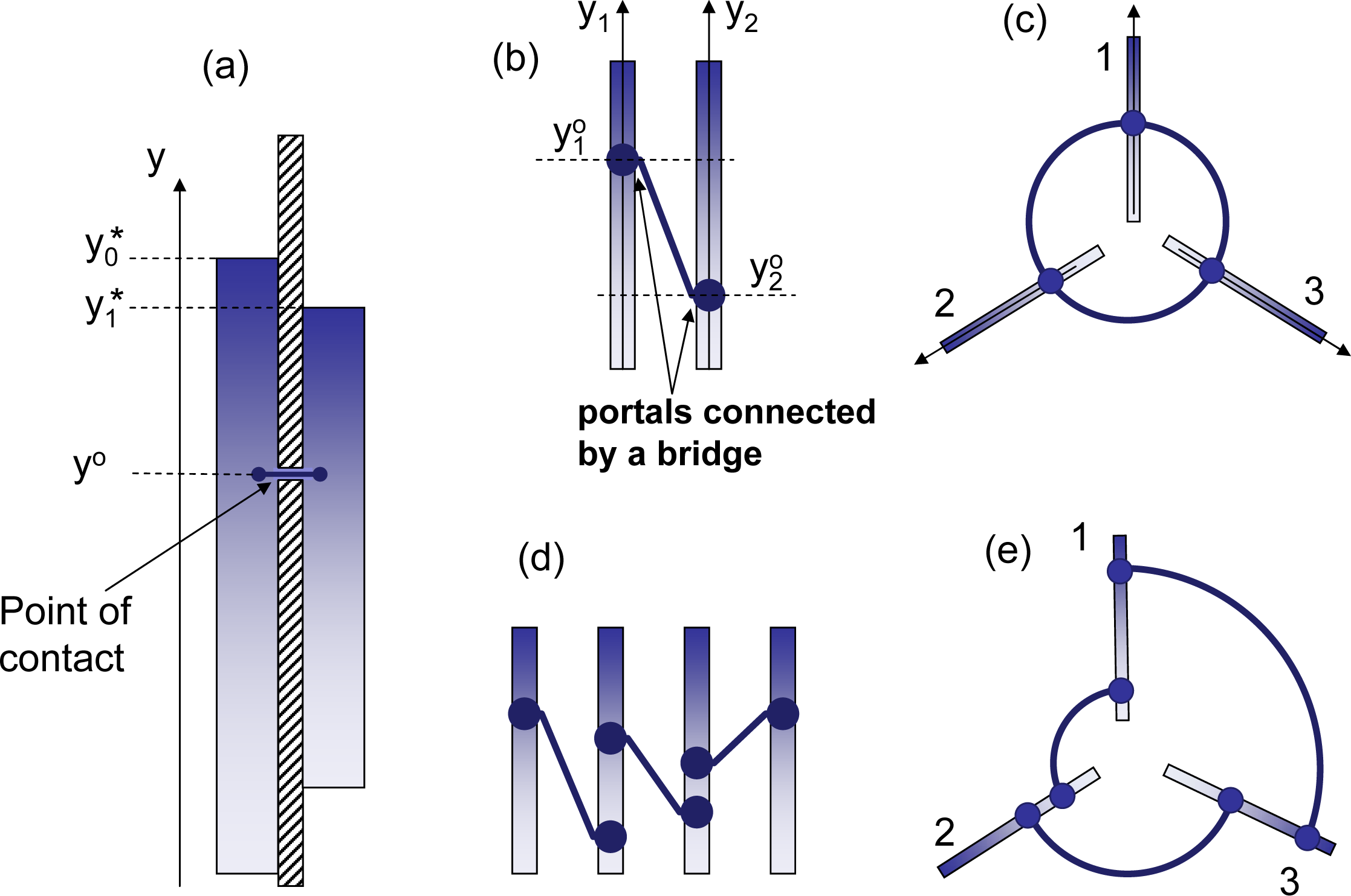
Connections through a point of contact can be given different interpretations. Figure 6a, shows two subsystems with the same property, y, that are connected at location y = y°. Another interpretation, which is illustrated in Figure 6b, is that y1 and y2 are internal properties of the subsystems, generally not related to each other, while the point of contact is an agreement that establishes the correspondence of two locations, and , that are called open portals. Particles can freely move between these portals through the bridge connecting the portals. Note that subsystems can have more than one open portal (see Figure 6d), as long as connections between these portals do not form a loop. Figure 6e illustrates such a loop that can make particle densities at two open portals that belong to a single subsystem inconsistent with each other. This would change the shapes of particle distributions ϕI(y) within the subsystems.
The case that is most interesting from the thermodynamic perspective is shown in Figure 6c: each subsystem has only one open portal: this ensures that the number of particles nI within each subsystem changes, while the subsystem distributions, ϕI(y), remain the same (presuming that each subsystem always converges to its internal steady state). Each portal can be connected to one or more of the portals that belong to the other subsystems. This connection is characterised by the subsystem particle numbers, nI, converging to their equilibrium values and by the detailed equilibrium between the subsystems (although the detailed balance is not necessarily achieved for the steady states within each subsystem). Assuming that the portal, , of subsystem I is connected to the portal, , of subsystem J, the equilibrium condition (40) is now rewritten as:
Let us consider how this equilibrium between K subsystems can be characterised by Tsallis entropy, which is defined as:
Maximisation of S is conducted first over for the shape of φI(y) under constraint:
Assuming that AI = 1 and all ZI are the same, we obtain and the following expression for the overall entropy:
7. Intransitivity, Transition to Complexity and the Risk/Benefit Dilemma
If competition becomes intransitive and intransitive triplets (4) exist, absolute ranking in not possible in such systems, and there is no absolute entropy (since the entropy potential is attached to the absolute ranking). Some intransitive systems may still retain local transitivity in smaller subdomains. In this case, the system may behave locally in the same way as transitive systems do, and it is still possible to use local absolute ranking and local entropy. In this case, the analog of the zeroth law of thermodynamics becomes invalid, allowing for the intransitivity of competitive potentials, such as χ1 ≺ χ2 ≺ χ3 ≺ χ1 (consider the subsystems I = 1, 2, 3 shown in Figure 5b, assuming that these subsystems are connected), and for cyclic evolutions. The system shown in Figure 1b is locally transitive and globally intransitive. Assuming that some positive mutations are present, this system evolves transitively in the vicinity of point A by escalating in the direction of increase of the local ranking, but the overall evolution appears to be cyclic, moving from A to B, then from B to C and, finally, from C back to A. When intransitivity becomes stronger (denser) and intransitive triplets can be found in the vicinity of any point, even local evolution of the system may become inconsistent with the principles of competitive thermodynamics. In complex systems, this evolution may result in competitive degradation (a process accompanied by slow, but noticeable, gradual decrease of competitiveness) and in competitive cooperation (the formation of structures with a reduced level of internal competition and violating the Stosszahlansatz). From the perspective of competitive thermodynamics, these processes are abnormal (see [1,9] for further discussion).
In this section, we consider a different example that involves punctuated evolution: for most of the time, the system seems to behave transitively and escalate towards higher ranks and higher entropy. This escalation is nevertheless punctuated by occasional crisis events, where the state of the system collapses to (or near to) the ground state. The system then repeats the slow growth/sudden collapse cycle. Note that only the cyclic component of evolution is considered here, while competitive evolutions may also involve a translational component (or components) and become spiral [9]. Cycles and collapses are common in real-world complex competitive systems of different kinds [16,17].
The present example of punctuated evolution is based on the risk/benefit dilemma (RBD): when comparing the available strategies, we would like to have low risk and high benefits; hence the problem has two parameters: the risk is denoted by y(1) and the benefit denoted by y(2). While high y(2) and low y(1) are most attractive, some compromises increasing the risk to increase the benefit or lowering the benefit to lower the risk may be necessary. When comparing two strategies, yA and yB, the choice is performed according to the following co-ranking:
One can easily see that choice RBD2 is transitive, allowing for absolute ranking:
Figure 7b shows the computational domain. The gray area y(2) > (y(1))1/3 is prohibited, reflecting the fact that one cannot have large benefits without being exposed to significant risks. The strategies superior with respect to A are in the small dark area, causing the system to evolve to higher risks and higher benefits. In the transitive case, the system grows to reach the equilibrium point maximising the absolute ranking, r(y), and then remains in the this state of relatively high benefits and reasonable risks forever. In intransitive case, the system does not stay in equilibrium, but collapses into a defensive strategy involving low risks and low benefits. The reason for this collapse is illustrated in Figure 7b. Aggressive strategy A is preferred over defensive strategy C, but as the system evolves even into a more aggressive strategy B, the risk associated with B becomes too high, and at a certain moment, defensive strategy C becomes more attractive than B. This results in the collapse of the growth and the rapid transition to defensive strategies.
For the transitive case, the entropy is defined by Equation (26). The translational case γ = 1 with the entropy potential depending linearly on ranking sy(y) = kr(y) is chosen. The parameters q = 1/Q = 1/1.2 and kq = 70 are selected to match the equilibrium distribution discussed below. The entropy definition takes the following form:
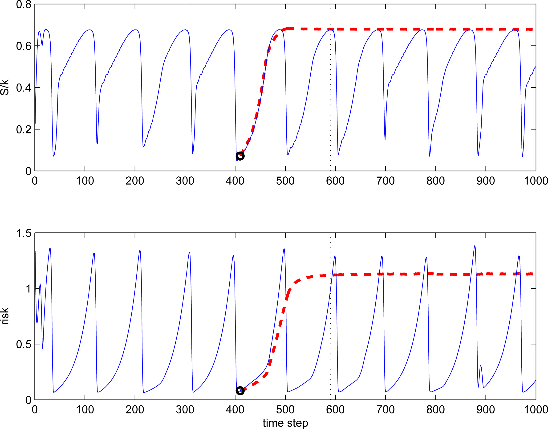
Figure 8 illustrates intransitive and transitive evolutions in the risk/benefit dilemma. The transitive branch is obtained by switching parameters from RBD1 to RBD2 at 410 time steps. The following intransitive and transitive evolutions seem to be very similar, but only up to a point, where maximal S is reached. The same definitions of ranking (57) and entropy (58) are used for both cases, transitive and intransitive. Then, the evolutions diverge: the transitive branch remains in an equilibrium state near the point of maximal entropy and maximal ranking, while the intransitive branch falls down into the region of defensive strategies. Video files covering these evolutions between steps 1 and 590 is offered as an electronic supplement to this article (see the Appendix for more details).
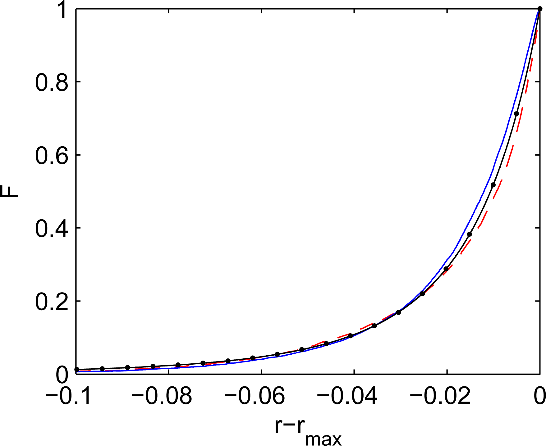
If the underlying competition rules and long-term history of the evolution are unknown, determining how a system is going to behave in the future by analysing the current distributions may be very difficult. Figure 9 illustrates this point. This figure shows the cdf of ranking r for transitive evolution (RBD2) and intransitive evolution (RBD1) at 590 time steps. Both distributions are very similar and can be approximated quite well by the q-exponential cdf (33) with Q = 1.2 and k/Q = 70.
The competitive mechanism represented by the risk/benefit dilemma can be one of the forces enacting economic cycles in the real world. From the economic perspective, the strategies reflected by RBD2 are seen as rational behaviours of individual players (say, investment agents). The benefit is represented by returns on investments, and ranking r is conventionally called utility in economics [18]. This utility weighs different factors against each other and enforces the transitivity of economic decisions. The intransitive strategies reflected by RBD1 would be seen by economists as semi-rational. Since risk and benefit do not represent directly comparable categories and the evaluation of risk is always subject to greater uncertainty, overlooking small risks and being overly concerned with high risks is a plausible economic strategy for any individual or company. While switching from the linear RBD2 to non-linear RBD1 seems like a minor adjustment for an economic element, it has a major effect on the functioning of the whole system: economic growth is interrupted by collapses, and the system evolves cyclically. Competition forces the competing elements to take higher and higher risks, until the risk becomes unsustainable.
8. Conclusions
In competitive systems with Gibbs mutations, the distributions tend to be exponential (assuming the isotropy of the property space). This case is described by the strongest similarity to conventional thermodynamics and the existence of detailed balance in the system. When the distribution of mutations deviates from that of Gibbs mutations, the q-exponents become very good approximations characterising the existence of long or short tails in the distributions caused by biases in taxing and supplying. In competitive thermodynamics, this corresponds to replacing conventional Boltzmann–Gibbs entropy by Tsallis entropy.
Unlike in conventional thermodynamics, competitive systems allow different types of equilibria possessing different degrees of similarity with the conventional thermodynamic equilibrium. Competition between subsystems without the exchange of mutations tends to be less stable than the connected equilibria, where subsystems exchange particles through both competition and mutations. Among connected equilibria, the case of Gibbs mutations bears the highest resemblance to conventional thermodynamics. When mutations are not of the Gibbs type, the point of contact equilibrium preserves this resemblance more than the other cases. The point of contact equilibrium has been analysed using Tsallis entropy. This analysis results in equilibrium conditions determined by the equivalence of competitive potentials. These potentials are linked to the introduced effective phase volumes of subsystems that depend on the location of the point of contact.
The thermodynamic analogy requires the transitivity of competition rules. In the case of intransitive competition rules, the system may behave anomalously when considered from the perspective of competitive thermodynamics. This involves the formation of structures, competitive degradations and cycles. The present work uses the example of the competitive risk/benefits dilemma and analyses the case of punctuated evolutions. For most of the time, the evolution of an intransitive competitive system, which represents the dilemma, closely resembles evolutions of transitive systems, which increase ranking and the associated entropy. At some moments, however, this evolution is punctuated and results in an abrupt collapse, which decreases ranking and the associated competitive entropy; this cannot possibly happen when the competition is transitive. Then, the system starts to grow and repeats the cycle again. While the consideration of competitive processes in this work is generic, similar behaviours can be found in biological, economic and other systems.
Video Supplements
entropy-16-00001-s001.avi entropy-16-00001-s002.aviAcknowledgments
The author thanks Bruce Littleboy for insightful discussions of economic issues. The author acknowledges funding by the Australian Research Council.
Conflicts of Interest
The authors declare no conflict of interest.
References
- Klimenko, A.Y. Mixing, entropy and competition. Phys. Scr 2012, 85, 068201. [Google Scholar]
- Tsallis, C. Nonextensive Statistical Mechanics and Thermodynamics: Historical Background and Present Status. In Nonextensive Statistical Mechanics and Its Applications; Abe, S., Okamoto, Y., Eds.; Springer: New York, NY, USA, 2001; pp. 3–98. [Google Scholar]
- Karev, G.P.; Koonin, E.V. Parabolic replicator dynamics and the principle of minimum Tsallis information gain. Biol. Direct 2013, 8, 19–19. [Google Scholar]
- Abe, S. General pseudoadditivity of composable entropy prescribed by the existence of equilibrium. Phys. Rev. E: Stat. Nonlinear Soft Matter Phys. 2001, 63, 061105. [Google Scholar]
- Abe, S. Heat and entropy in nonextensive thermodynamics: Transmutation from Tsallis theory to Renyi-entropy-based theory. Phys. A Stat. Mech. Appl 2001, 300, 417–423. [Google Scholar]
- Tsallis, C.; Mendes, R.; Plastino, A.R. The role of constraints within generalized nonextensive statistics. Phys. A Stat. Mech. Appl 1998, 261, 534–554. [Google Scholar]
- Hanel, R.; Thurner, S. When do generalized entropies apply? How phase space volume determines entropy. EPL (Europhys. Lett.) 2011, 96, 50003. [Google Scholar]
- Gould, S.J.; Eldredge, N. Punctuated equilibrium comes of age. Nature 1993, 366, 223–227. [Google Scholar]
- Klimenko, A.Y. Complex competitive systems and competitive thermodynamics. Phil. Trans. R. Soc. A 2013. [Google Scholar] [CrossRef]
- Klimenko, A.Y. Conservative and competitive mixing and their applications. Phys. Scr 2010, T142, 014054. [Google Scholar]
- Klimenko, A.Y.; Pope, S.B. Propagation speed of combustion and invasion waves in stochastic simulations with competitive mixing. Combust. Theory Modell 2012, 16, 679–714. [Google Scholar]
- Ohta, T. Extension to the Neutral Mutation Random Drift Hypothesis. In Molecular Evolution and Polymorphism; Kimura, M., Ed.; National Institute of Genetics: Mishima, Japan, 1977; pp. 148–167. [Google Scholar]
- Wonnapinij, P.; Chinnery, P.F.; Samuels, D.C. The distribution of mitochondrial DNA heteroplasmy due to random genetic drift. Am. J. Hum. Genet 2008, 83, 582–593. [Google Scholar]
- Finsterer, J. Manifestations of the mitochondrial A3243G mutation. Int. J. Cardiol 2009, 137, 60–62. [Google Scholar]
- Klimenko, A.Y. Teaching the third law of thermodynamics. Open Thermodyn. J 2012, 6, 1–14. [Google Scholar]
- Klimenko, A.Y. Technological Cycles their impact on Science, Engineering and Engineering Education. Int. J. Tech. Knowl. Soc 2008, 4, 11–18. [Google Scholar]
- Grudin, J. Punctuated Equilibrium and Technology Change. Interactions 2012, 19, 62–66. [Google Scholar]
- Candeal, J.C.; de Miguel, J.R.; Indurain, E.; Mehta, G. Utility and entropy. Econ. Theory 2001, 17, 233–238. [Google Scholar]
Appendix Video Files with the Simulations of the Risk/Benefit Dilemma
Simulations of the cases, RBD1 and RBD2, involving 10,000 Pope particles are offered as video supplements to this article:
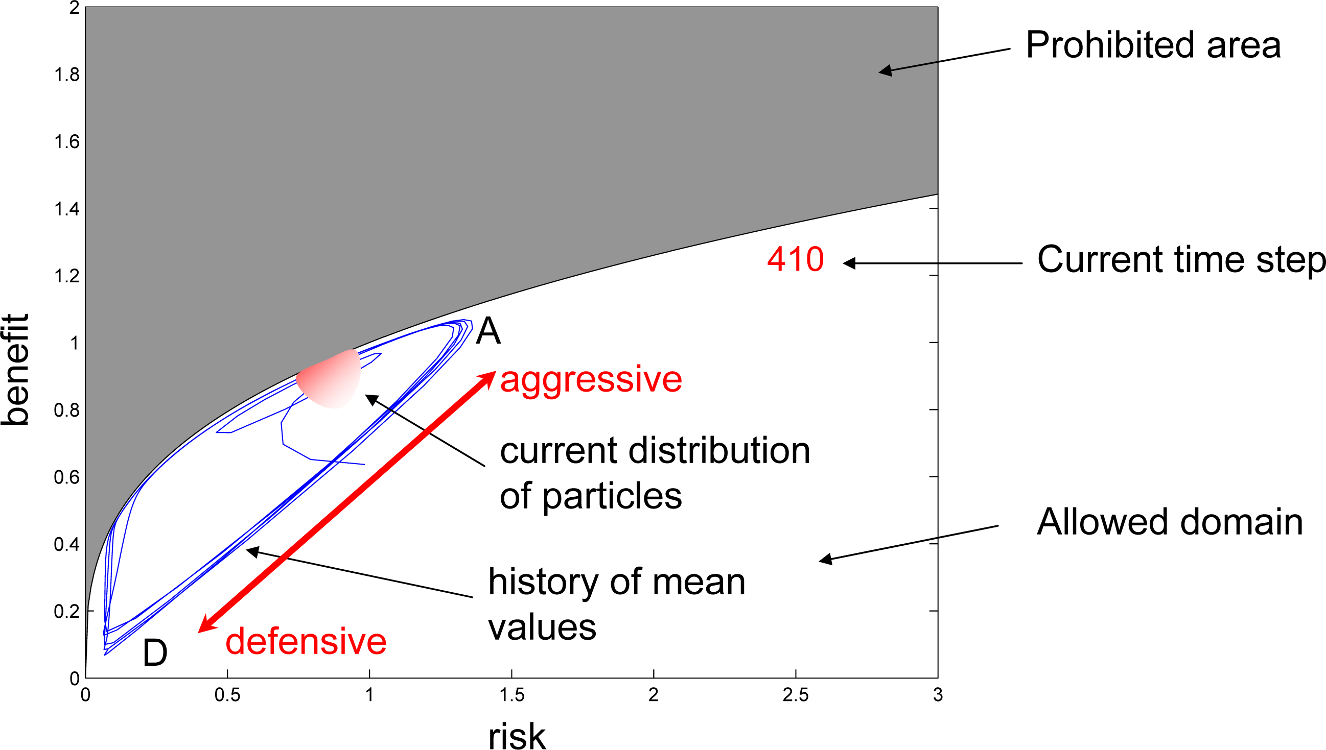
Competition is intransitive in RBD1 and transitive in RBD2. The cases are branched apart at 410 time steps with the same distribution of particles. The format of the videos is explained in Figure A1. In the intransitive simulations of the risk/benefits dilemma, competition forces competitors to undertake more and more aggressive strategies, while the distribution moves from D to A. This leads to unsustainably high risk and the punctuation of continuous evolution by a sudden collapse of the system by elements seeking refuge in defensive strategies near D. While the evolution is punctuated in the intransitive case, the transitive version of the simulations safely reaches equilibrium and remains there forever. In spite of principal differences, the ascending fragments of both simulations are very similar.


© 2014 by the authors; licensee MDPI, Basel, Switzerland This article is an open access article distributed under the terms and conditions of the Creative Commons Attribution license (http://creativecommons.org/licenses/by/3.0/).
Share and Cite
Klimenko, A.Y. Entropy and Equilibria in Competitive Systems. Entropy 2014, 16, 1-22. https://doi.org/10.3390/e16010001
Klimenko AY. Entropy and Equilibria in Competitive Systems. Entropy. 2014; 16(1):1-22. https://doi.org/10.3390/e16010001
Chicago/Turabian StyleKlimenko, A. Y. 2014. "Entropy and Equilibria in Competitive Systems" Entropy 16, no. 1: 1-22. https://doi.org/10.3390/e16010001
APA StyleKlimenko, A. Y. (2014). Entropy and Equilibria in Competitive Systems. Entropy, 16(1), 1-22. https://doi.org/10.3390/e16010001