Objective Bayesianism and the Maximum Entropy Principle

Abstract

Objective Bayesian epistemology invokes three norms: the strengths of our beliefs should be probabilities; they should be calibrated to our evidence of physical probabilities; and they should otherwise equivocate sufficiently between the basic propositions that we can express. The three norms are sometimes explicated by appealing to the maximum entropy principle, which says that a belief function should be a probability function, from all those that are calibrated to evidence, that has maximum entropy. However, the three norms of objective Bayesianism are usually justified in different ways. In this paper, we show that the three norms can all be subsumed under a single justification in terms of minimising worst-case expected loss. This, in turn, is equivalent to maximising a generalised notion of entropy. We suggest that requiring language invariance, in addition to minimising worst-case expected loss, motivates maximisation of standard entropy as opposed to maximisation of other instances of generalised entropy. Our argument also provides a qualified justification for updating degrees of belief by Bayesian conditionalisation. However, conditional probabilities play a less central part in the objective Bayesian account than they do under the subjective view of Bayesianism, leading to a reduced role for Bayes’ Theorem.

1. Introduction

Objective Bayesian epistemology is a theory about the strength of belief. As formulated by Williamson [1], it invokes three norms:

• Probability: The strengths of an agent’s beliefs should satisfy the axioms of probability. That is, there should be a probability function, $P_E:S\mathcal{L}⟶[0,1]$, such that for each sentence θ of the agent’s language $\mathcal{L}$, $P_E(\theta )$ measures the degree to which the agent with evidence E believes sentence θ. (Here, $\mathcal{L}$ will be construed as a finite propositional language and $S\mathcal{L}$ as the set of sentences of $\mathcal{L}$, formed by recursively applying the usual connectives.)
• Calibration: The strengths of an agent’s beliefs should satisfy constraints imposed by her evidence E. In particular, if the evidence determines just that physical probability (aka chance), $P^{*}$, is in some set ${\mathbb{P}}^{*}$ of probability functions defined on $S\mathcal{L}$, then $P_E$ should be calibrated to physical probability insofar as it should lie in the convex hull, $\mathbb{E}=⟨{\mathbb{P}}^{*}⟩$, of the set ${\mathbb{P}}^{*}$. (We assume throughout this paper that chance is probabilistic, i.e., that $P^{*}$ is a probability function.)
• Equivocation: The agent should not adopt beliefs that are more extreme than is demanded by her evidence E. That is, $P_E$ should be a member of $\mathbb{E}$ that is sufficiently close to the equivocator function, $P_{=}$, which gives the same probability to each $\omega \in \Omega$, where the state descriptions or states, ω, are sentences describing the most fine-grained possibilities expressible in the agent’s language.

One way of explicating these norms proceeds as follows. Measure closeness of $P_E$ to the equivocator by Kullback-Leibler divergence, $d(P_E,P_{=})={\sum }_{\omega \in \Omega }{P}_E(\omega )log\frac{P_E(\omega )}{P_{=}(\omega )}$. Then, if there is some function in $\mathbb{E}$ that is closest to the equivocator, $P_E$ should be such a function. If $\mathbb{E}$ is closed, then there is guaranteed to be some function in $\mathbb{E}$ closest to the equivocator; as $\mathbb{E}$ is convex, there is at most one such function. Then we have the maximum entropy principle [2]: $P_E$ is the function in $\mathbb{E}$ that has maximum entropy H, where $H(P)=-{\sum }_{\omega \in \Omega }P(\omega )logP(\omega )$.

The question arises as to how the three norms of objective Bayesianism should be justified, and whether the maximum entropy principle provides a satisfactory explication of the norms.

The probability norm is usually justified by a Dutch book argument. Interpret the strength of an agent’s belief in θ to be a betting quotient, i.e., a number x, such that the agent is prepared to bet $xS$ on θ with return S if θ is true, where S is an unknown stake, positive or negative. Then the only way to avoid the possibility that stakes may be chosen so as to force the agent to lose money, whatever the true state of the world, is to ensure that the betting quotients satisfy the axioms of probability (see e.g., Theorem 3.2 in [1]).

The calibration norm may be justified by a different sort of betting argument. If the agent bets repeatedly on sentences with known chance y with some fixed betting quotient x, then she is sure to lose money in the long run unless $x=y$ (see, e.g., pp. 40–41 in [1]). Alternatively, on a single bet with known chance y, the agent’s expected loss is positive unless her betting quotient $x=y$, where the expectation is determined with respect to the chance function $P^{*}$ (pp. 41–42 in [1]). More generally, if evidence E determines that $P^{*}\in {\mathbb{P}}^{*}$ and the agent makes such bets, then sure loss/positive expected loss can be forced unless $P_E\in ⟨{\mathbb{P}}^{*}⟩$.

The equivocation norm may be justified by appealing to a third notion of loss. In the absence of any particular information about the loss $L(\omega ,P)$ one incurs when one’s strengths of beliefs are represented by P and ω turns out to be the true state, one can argue that one should take the loss function L to be logarithmic, $L(\omega ,P)=-logP(\omega )$ (pp. 64–65 in [1]). Then the probability function P that minimises the worst case expected loss, subject to the information that $P^{*}\in \mathbb{E}$, where $\mathbb{E}$ is closed and convex, is simply the probability function $P\in \mathbb{E}$ closest to the equivocator—equivalently, the probability function in $\mathbb{E}$ that has maximum entropy [3,4].

The advantage of these three lines of justification is that they make use of the rather natural connection between strength of belief and betting. This connection was highlighted by Frank Ramsey:

All our lives, we are in a sense betting. Whenever we go to the station, we are betting that a train will really run, and if we had not a sufficient degree of belief in this, we should decline the bet and stay at home.

(p. 183 in [5])

The problem is that the three norms are justified in rather different ways. The probability norm is motivated by avoiding sure loss. The calibration norm is motivated by avoiding sure long-run loss or by avoiding positive expected loss. The equivocation norm is motived by minimising worst-case expected loss. In particular, the loss function appealed to in the justification of the equivocation norm differs from that invoked by the justifications of the probability and calibration norms.

In this paper, we seek to rectify this problem. That is, we seek a single justification of the three norms of objective Bayesian epistemology.

The approach we take is to generalise the justification of the equivocation norm, outlined above, in order to show that only the strengths of beliefs that are probabilistic, calibrated and equivocal minimise worst-case expected loss. We shall adopt the following starting point: as discussed above, $\mathbb{E}=⟨{\mathbb{P}}^{*}⟩$ is taken to be convex and non-empty throughout this paper; we shall also assume that the strengths of the agent’s beliefs can be measured by non-negative real numbers—an assumption that is rejected by advocates of imprecise probability, a position that we will discuss separately in Section 5.3. We do not assume throughout that $\mathbb{E}$ is such that it admits some function that has maximum entropy—e.g., that $\mathbb{E}$ is closed—but we will be particularly interested in the case in which $\mathbb{E}$ does contain its entropy maximiser, in order to see whether some version of the maximum entropy principle is justifiable in that case.

In Section 2, we shall consider the scenario in which the agent’s belief function, $\mathit{bel}$, is defined over propositions, i.e., sets of possible worlds. Using ω to denote a possible world as well as the state of $\mathcal{L}$ that picks out that possible world, we have that $\mathit{bel}$ is a function from the power set of a finite set Ω of possible worlds ω to the non-negative real numbers, $\mathit{bel}:\mathcal{P}\Omega ⟶{\mathbb{R}}_{\ge 0}$. When it comes to justifying the probability norm, this will give us enough structure to show that degrees of belief should be additive. Then, in Section 3, we shall consider the richer framework in which the belief function is defined over sentences, i.e., $\mathit{bel}:S\mathcal{L}⟶{\mathbb{R}}_{\ge 0}$. This will allow us to go further by showing that different sentences that express the same proposition should be believed to the same extent. In Section 4, we shall explain how the preceding results can be used to motivate a version of the maximum entropy principle. In Section 5, we draw out some of the consequences of our results for Bayes’ theorem. In particular, conditional probabilities and Bayes’ theorem play a less central role under this approach than they do under subjective Bayesianism. Furthermore, in Section 5 we relate our work to the imprecise probability approach and suggest that the justification of the norms of objective Bayesianism presented here can be reinterpreted in a non-pragmatic way.

The key results of the paper are intended to demonstrate the following points. Theorem 1 (which deals with beliefs defined over propositions) and Theorem 4 (respectively, belief over sentences) show that only a logarithmic loss function satisfies certain desiderata that, we suggest, any default loss function should satisfy. This allows us to focus our attention on logarithmic loss. Theorems 2, 3 (for propositions) and Theorems 5, 6 (for sentences) show that minimising worst-case expected logarithmic loss corresponds to maximising a generalised notion of entropy. Theorem 7 justifies maximising standard entropy, by viewing this maximiser as a limit of generalised entropy maximisers. Theorem 9 demonstrates a level of agreement between updating beliefs by Bayesian conditionalisation and updating by maximising generalised entropy. Theorem 10 shows that the generalised notion of entropy considered in this paper is pitched at precisely the right level of generalisation.

Three appendices to the paper help to shed light on the generalised notion of entropy introduced in this paper. Appendix A motivates the notion by offering justifications of generalised entropy that mirror Shannon’s original justification of standard entropy. Appendix B explores some of the properties of the functions that maximise generalised entropy. Appendix C justifies the level of generalisation of entropy to which we appeal.

2. Belief over Propositions

In this section, we shall show that if a belief function defined on propositions is to minimise worst-case expected loss, then it should be a probability function, calibrated to physical probability, which maximises a generalised notion of entropy. The argument will proceed in several steps. As a technical convenience, in Section 2.1, we shall normalise the belief functions under consideration. In Section 2.2, we introduce the appropriate generalisation of entropy. In Section 2.3, we argue that, by default, loss should be taken to be logarithmic. Then, in Section 2.4, we introduce scoring rules, which measure expected loss. Finally, in Section 2.5, we show that worst-case expected loss is minimised just when generalised entropy is maximised.

For the sake of concreteness, we will take Ω to be generated by a propositional language, $\mathcal{L}=\{A_1,\dots ,A_n\}$, with propositional variables, $A_1,\dots ,A_n$. The states, ω, take the form ${}_{\pm }{A}_1\wedge \cdots \wedge {}_{\pm }{A}_n$, where $+A_i$ is just $A_i$ and $-A_i$ is $\neg A_i$. Thus, there are $2^n$ states, $\omega \in \Omega =\{{}_{\pm }{A}_1\wedge \cdots \wedge {}_{\pm }{A}_n\}$. We can think of each such state as representing a possible world. A proposition (or, in the terminology of the mathematical theory of probability, an ‘event’) may be thought of as a subset of Ω, and a belief function, $\mathit{bel}:\mathcal{P}\Omega ⟶{\mathbb{R}}_{\ge 0}$, thus assigns a degree of belief to each proposition that can be expressed in the agent’s language. For a proposition $F\subseteq \Omega$, we will use $\overline{F}$ to denote $\Omega \setminus F$. $|F|$ denotes the size of proposition $F\subseteq \Omega$, i.e., the number of states under which it is true.

Let Π be the set of partitions of Ω; a partition $\pi \in \Pi$ is a set of mutually exclusive and jointly exhaustive propositions. To control the proliferation of partitions, we shall take the empty set, ∅, to be contained only in one partition, namely $\{\Omega ,\varnothing \}$.

2.1. Normalisation

There are finitely many propositions ($\mathcal{P}\Omega$ has $2^{2^n}$ members), so any particular belief function, $\mathit{bel}$, takes values in some interval $[0,M]\subseteq {\mathbb{R}}_{\ge 0}$. It is just a matter of convention as to the scale on which belief is measured, i.e., as to what upper bound M we might consider. For convenience, we shall normalise the scale to the unit interval, $[0,1]$, so that all belief functions are considered on the same scale.

Definition 1 (Normalised belief function on propositions). Let $M={max}_{\pi \in \Pi }{\sum }_{F\in \pi }\mathit{bel}(F)$. Given a belief function, $\mathit{bel}:\mathcal{P}\Omega ⟶{\mathbb{R}}_{\ge 0}$, that is not zero everywhere, its normalisation, $B:\mathcal{P}\Omega ⟶[0,1]$, is defined by setting $B(F)=\mathit{bel}(F)/M$ for each $F\subseteq \Omega$. We shall denote the set of normalised belief functions by $\mathbb{B}$, so:

$$\begin{array}{c}\hfill \mathbb{B}=\{B:\mathcal{P}\Omega ⟶[0,1]:\sum _{F\in \pi }B(F)\le 1\text{ for all }\pi \in \Pi \text{ and }\sum _{F\in \pi }B(F)=1\text{ for some }\pi \}\end{array}$$

Without loss of generality, we rule out of consideration the non-normalised belief function that gives zero degree of belief to each proposition; it will become clear in Section 2.4 that this belief function is of little interest, as it can never minimise worst-case expected loss. For purely technical convenience, we will often consider the convex hull, $⟨\mathbb{B}⟩$, of $\mathbb{B}$. In which case, we rule into consideration certain belief functions that are not normalised, but which are convex combinations of normalised belief functions. Henceforth, then, we shall focus our attention on belief functions in $\mathbb{B}$ and $⟨\mathbb{B}⟩$.

Note that we do not impose any further restrictions on the agent’s belief function—such as additivity; or the requirement that $B(G)\le B(F)$ whenever $G\subseteq F$; or that the empty proposition, ∅, has belief zero; or the sure proposition, Ω, is assigned belief of one. Our aim is to show that belief functions that do not satisfy such conditions will expose the agent to avoidable loss.

For any $B\in ⟨\mathbb{B}⟩$ and every $F\subseteq \Omega$, we have $B(F)+B(\overline{F})\le 1$, because $\{F,\overline{F}\}$ is a partition. Indeed:

$$\begin{array}{cc}\hfill \sum _{F\subseteq \Omega }B(F)& =\frac{1}{2}·\left(\sum _{F\subseteq \Omega }B(F)+\sum _{F\subseteq \Omega }B(\overline{F})\right)\le \frac{1}{2}·|\mathcal{P}\Omega |=2^{2^n-1}\hfill \end{array}$$

(1)

Recall that a subset of ${\mathbb{R}}^N$ is compact, if and only if it is closed and bounded.

Lemma 1 (Compactness). $\mathbb{B}$ and $⟨\mathbb{B}⟩$ are compact.

Proof: $\mathbb{B}\subset {\mathbb{R}}^{|\mathcal{P}\Omega |}$ is bounded, where ⊂ denotes strict subset inclusion. Now, consider a sequence, ${(B_t)}_{t\in \mathbb{N}}\in \mathbb{B}$ which converges to some $B\in {\mathbb{R}}^{|\mathcal{P}\Omega |}.$ Then, for all $\pi \in \Pi$, we find ${\sum }_{F\in \pi }B(F)\le 1.$ Assume that $B\notin \mathbb{B}$. Thus for all $\pi \in \Pi$, we have ${\sum }_{F\in \pi }B(F)<1.$ However, then there has to exist a $t_0\in \mathbb{N}$, such that for all $t\ge t_0$ and all $\pi \in \Pi$, ${\sum }_{F\in \pi }{B}_t(F)<1$. This contradicts $B_t\in \mathbb{B}.$ Thus, $\mathbb{B}$ is closed and, hence, compact.

$⟨\mathbb{B}⟩$ is the convex hull of a compact set. Hence, $⟨\mathbb{B}⟩\subset {\mathbb{R}}^{|\mathcal{P}\Omega |}$ is closed and bounded and so compact. ■

We will be particularly interested in the subset, $\mathbb{P}\subseteq \mathbb{B}$, of belief functions defined by:

$$\mathbb{P}=\{B:\mathcal{P}\Omega ⟶[0,1]:\sum _{F\in \pi }B(F)=1\text{ for all }\pi \in \Pi \}$$

(2)

$\mathbb{P}$ is the set of probability functions:

Proposition 1. $P\in \mathbb{P}$ if and only if $P:\mathcal{P}\Omega ⟶[0,1]$ satisfies the axioms of probability:

P1:

$P(\Omega )=1$ and $P(\varnothing )=0$.

P2:

If $F\cap G=\varnothing$, then $P(F)+P(G)=P(F\cup G)$.

Proof: Suppose $P\in \mathbb{P}$. $P(\Omega )=1$, because $\{\Omega \}$ is a partition. $P(\varnothing )=0$, because $\{\Omega ,\varnothing \}$ is a partition and $P(\Omega )=1$. If $F,G\subseteq \Omega$ are disjoint, then $P(F)+P(G)=P(F\cup G)$, because $\{F,G,\overline{F\cup G}\}$ and $\{F\cup G,\overline{F\cup G}\}$ are both partitions, so $P(F)+P(G)=1-P(\overline{F\cup G})=P(F\cup G)$.

On the other hand, suppose P1 and P2 hold. ${\sum }_{F\in \pi }P(F)=1$ can be seen by induction on the size of π. If $|\pi |=1$, then $\pi =\{\Omega \}$ and $P(\Omega )=1$ by P1. Suppose, then, that $\pi =\{F_1,\dots ,F_{k+1}\}$ for $k\ge 1$. Now, ${\sum }_{i=1}^{k-1}P(F_i)+P(F_k\cup F_{k+1})=1$ by the induction hypothesis and $P(F_k\cup F_{k+1})=P(F_k)+P(F_{k+1})$ by P2, so ${\sum }_{F\in \pi }P(F)=1$, as required.  ■

Example 1 (Contrasting $\mathbb{B}$ with $\mathbb{P}$). Using Equation (1), we find ${\sum }_{F\subseteq \Omega }P(F)=\frac{|\mathcal{P}\Omega |}{2}\ge {\sum }_{F\subseteq \Omega }B(F)$ for all $P\in \mathbb{P}$ and $B\in \mathbb{B}.$ For probability functions, $P\in \mathbb{P}$, probability is evenly distributed among the propositions of fixed size in the following sense:

$$\begin{array}{cc}\hfill \sum _{\begin{array}{c}F\subseteq \Omega \\ |F|=t\end{array}}P(F)& =\sum _{\omega \in \Omega }P(\omega )·|\{F\subseteq \Omega :|F|=t\text{ and }\omega \in F\}|\hfill \end{array}$$

(3)

$$\begin{array}{cc}& =\sum _{\omega \in \Omega }P(\omega )\left(\genfrac{}{}{0pt}{}{|\Omega |-1}{t-1}\right)=\left(\genfrac{}{}{0pt}{}{|\Omega |-1}{t-1}\right)\hfill \end{array}$$

(4)

where $P(\omega )$ abbreviates $P(\{\omega \}).$ For $B\in \mathbb{B}$ and $t>\frac{|\Omega |}{2}\ge 2$, we have, in general, only the following inequality:

$$\begin{array}{c}\hfill 0\le \sum _{\begin{array}{c}F\subseteq \Omega \\ |F|=t\end{array}}B(F)\le |\{F\subseteq \Omega :|F|=t\}|=\left(\genfrac{}{}{0pt}{}{|\Omega |}{t}\right)\end{array}$$

(5)

For $B_1\in \mathbb{B}$, defined as $B_1(\omega )=1$, for some specific ω, and $B_1(F)=0$ for all other $F\subseteq \Omega$, we have that the lower bound is tight. For $B_2\in \mathbb{B}$, defined as $B_2(F)=1$, for $|F|=t$, and $B_2(F)=0$, for all other $F\subseteq \Omega$, the upper bound is tight.

To illustrate the potentially uneven distribution of beliefs for a $B\in \mathbb{B},$ let $A_1,A_2$ be the propositional variables in $\mathcal{L},$ so Ω contains four elements. Now, consider the $B\in \mathbb{B}$ such that $B(\varnothing )=0,$ $B(F)=\frac{1}{100}$ for $|F|=1,$ $B(F)=\frac{1}{2}$ for $|F|=2,$ $B(F)=\frac{99}{100}$ for $|F|=3$ and $B(\Omega )=1.$ Note, in particular, that there is no $P\in \mathbb{P}$ such that $B(F)\le P(F)$ for all $F\subseteq \Omega .$

2.2. Entropy

The entropy of a probability function is standardly defined as:

$$H_{\Omega }(P):=-\sum _{\omega \in \Omega }P(\omega )logP(\omega )$$

(6)

We shall adopt the usual convention that $-xlog0=x·\infty =\infty$, if $x>0$ and $0log0=0$.

We will need to extend the standard notion of entropy to apply to normalised belief functions, not just to probability functions. Note that the standard entropy only takes into account those propositions that are in the partition $\{\{\omega \}:\omega \in \Omega \}$ which partitions Ω into states. This is appropriate when entropy is applied to probability functions, because a probability function is determined by its values on the states. However, this is not appropriate if entropy is to be applied to belief functions: in that case, one cannot simply disregard all those propositions that are not in the partition of Ω into states—one needs to consider propositions in other partitions, too. In fact, there are a range of entropies of a belief function, according to how much weight is given to each partition π in the entropy sum:

Definition 2 (g-entropy). Given a weighting function $g:\Pi ⟶{\mathbb{R}}_{\ge 0}$, the generalised entropy or g-entropy of a normalised belief function is defined as:

$$H_g(B):=-\sum _{\pi \in \Pi }g(\pi )\sum _{F\in \pi }B(F)logB(F)$$

(7)

The standard entropy, $H_{\Omega }$, corresponds to $g_{\Omega }$-entropy, where

$$g_{\Omega }(\pi )=\left\{\begin{array}{ccc}1& :& \pi =\{\{\omega \}:\omega \in \Omega \}\hfill \\ 0& :& \text{otherwise}\hfill \end{array}\right.$$

(8)

We can define the partition entropy, $H_{\Pi }$, to be the $g_{\Pi }$-entropy, where $g_{\Pi }(\pi )=1$ for all $\pi \in \Pi$. Then:

$$\begin{array}{ccc}\hfill H_{\Pi }(B)& =& -\sum _{\pi \in \Pi }\sum _{F\in \pi }B(F)logB(F)\hfill \\ & =& -\sum _{F\subseteq \Omega }\mathit{par}(F)B(F)logB(F)\hfill \end{array}$$

(9)

where $\mathit{par}(F)$ is the number of partitions in which F occurs. Note that according to our convention, $\mathit{par}(\varnothing )=1$ and $\mathit{par}(\Omega )=2$, because Ω occurs in partitions, $\{\varnothing ,\Omega \}$ and $\{\Omega \}$. Otherwise, $\mathit{par}(F)=b_{|\overline{F}|}$, where $b_k:={\sum }_{i=1}^{k}1/i!{\sum }_{j=0}^i{(-1)}^{i-j}\left(\genfrac{}{}{0pt}{}{i}{j}\right)j^k$ is the k’th Bell number, i.e., the number of partitions of a set of k elements.

We can define the proposition entropy $H_{\mathcal{P}\Omega }$ to be the $g_{\mathcal{P}\Omega }$-entropy, where

$$g_{\mathcal{P}\Omega }(\pi )=\left\{\begin{array}{ccc}1& :& |\pi |=2\hfill \\ 0& :& \text{otherwise}\hfill \end{array}\right.$$

(10)

Then:

$$\begin{array}{ccc}\hfill H_{\mathcal{P}\Omega }(B)& =& -\sum _{\pi \in \Pi }\sum _{\begin{array}{c}F\in \pi \\ |\pi |=2\end{array}}B(F)logB(F)\hfill \\ & =& -\sum _{F\subseteq \Omega }B(F)logB(F)\hfill \end{array}$$

(11)

In general, we can express $H_g(B)$ in the following way, which reverses the order of the summations:

$$H_g(B)=-\sum _{F\subseteq \Omega }\left(\sum _{\begin{array}{c}\pi \in \Pi \\ F\in \pi \end{array}}g(\pi )\right)B(F)logB(F)$$

(12)

As noted above, one might reasonably demand of a measure of the entropy of a belief function that each belief should contribute to the entropy sum, i.e., for each $F\subseteq \Omega$, ${\sum }_{\begin{array}{c}\pi \in \Pi \\ F\in \pi \end{array}}g(\pi )\ne 0$:

Definition 3 (Inclusive weighting function). A weighting function $g:\Pi ⟶{\mathbb{R}}_{\ge 0}$ is inclusive if for all $F\subseteq \Omega$, there is some partition π containing F such that $g(\pi )>0$.

This desideratum rules out the standard entropy in favour of other candidate measures, such as the partition entropy and the proposition entropy.

We have seen so far that g-entropy is a natural generalisation of standard entropy from probability functions to belief functions. In Section 2.5, we shall see that g-entropy is of particular interest, because maximising g-entropy corresponds to minimising worst-case expected loss—this is our main reason for introducing the concept. However, there is a third reason why g-entropy is of interest. Shannon (§6 in [6]) provided an axiomatic justification of standard entropy as a measure of the uncertainty encapsulated in a probability function. Interestingly, as we show in Appendix A, Shannon’s argument can be adapted to give a justification of our generalised entropy measure. Thus, g-entropy can also be thought of as a measure of the uncertainty of a belief function.

In the remainder of this section, we will examine some of the properties of g-entropy.

Lemma 2. The function $-log:[0,1]\to [0,\infty ]$ is continuous in the standard topology on ${\mathbb{R}}_{\ge 0}\cup \{+\infty \}.$

Proof: To obtain the standard topology on ${\mathbb{R}}_{\ge 0}\cup \{+\infty \}$, take as open sets infinite unions and finite intersections over the open sets of ${\mathbb{R}}_{\ge 0}$ and sets of the form, $(r,\infty ]$, where $r\in \mathbb{R}.$ In this topology on $[0,\infty ],$ a set $M\subseteq {\mathbb{R}}_{\ge 0}$ is open if and only if it is open in the standard topology in ${\mathbb{R}}_{\ge 0}.$ Hence, $-log$ is continuous in this topology on $(0,1].$

Let ${(a_t)}_{t\in \mathbb{N}}$ be a sequence in $[0,1]$ with limit zero. For all $ϵ>0$, there exists a $T\in \mathbb{N}$ such that $-log{a}_t>\frac{1}{ϵ}$ for all $t>T.$ Hence, for all open sets U containing $+\infty$, there exists a K such that $-log{a}_m\in U$ if $m>K.$ Therefore, $-log{a}_t$ converges to $+\infty .$ Thus, ${lim}_{t\to \infty }-log{a}_t=+\infty =-log{lim}_{t\to \infty }{a}_t.$  ■

Proposition 2. g-entropy is non-negative and, for inclusive g, strictly concave on $⟨\mathbb{B}⟩$.

Proof: $B(F)\in [0,1]$ for all F, so $logB(F)\le 0$, and $g(\pi ){\sum }_{F\in \pi }B(F)logB(F)\le 0$. Hence, ${\sum }_{\pi \in \Pi }-g(\pi ){\sum }_{F\in \pi }B(F)logB(F)\ge 0,$ i.e., g-entropy is non-negative.

Take distinct $B_1,B_2\in ⟨\mathbb{B}⟩$ and $\lambda \in (0,1)$, and let $B=\lambda B_1+(1-\lambda )B_2$. Now, $xlogx$ is strictly convex on $[0,1]$, i.e.,

$$B(F)logB(F)\le \lambda B_1(F)log{B}_1(F)+(1-\lambda )B_2(F)log{B}_2(F)$$

(13)

with equality just when $B_1(F)=B_2(F)$.

Consider an inclusive weighting function, g.

$$\begin{array}{ccc}\hfill H_g(\lambda B_1+(1-\lambda )B_2)& =& -\sum _{\pi \in \Pi }g(\pi )\sum _{F\in \pi }B(F)logB(F)\hfill \\ & \ge & -\sum _{\pi \in \Pi }g(\pi )\sum _{F\in \pi }\left(\lambda B_1(F)log{B}_1(F)+(1-\lambda )B_2(F)log{B}_2(F)\right)\hfill \\ & =& \lambda H_g(B_1)+(1-\lambda )H_g(B_2)\hfill \end{array}$$

(14)

with equality iff for all F, $B_1(F)=B_2(F)$, since g is inclusive. However, $B_1$ and $B_2$ are distinct, so equality does not obtain. In other words, g-entropy is strictly concave.  ■

Corollary 1. For inclusive g, if g-entropy is maximised by a function $P^{†}$ in convex $\mathbb{E}\subseteq \mathbb{P}$, it is uniquely maximised by $P^{†}$ in $\mathbb{E}$.

Corollary 2. For inclusive g, g-entropy is uniquely maximised in the closure, $\left[\mathbb{E}\right]$, of $\mathbb{E}$.

If g is not inclusive, concavity is not strict. For example, if the standard entropy, $H_{\Omega }$, is maximised by $B^{†}$, then it is also maximised by any belief function $C^{†}$ that agrees with $B^{†}$ on the states $\omega \in \Omega$.

Note that different g-entropy measures can have different maximisers on a convex subset $\mathbb{E}$ of probability functions. For example, when $\Omega =\{{\omega }_1,{\omega }_2,{\omega }_3,{\omega }_4\}$ and $\mathbb{E}=\{P\in \mathbb{P}:P({\omega }_1)+2.75P({\omega }_2)+7.1P({\omega }_3)=1.7,P({\omega }_4)=0\}$, then the proposition entropy maximiser, the standard entropy maximiser and the partition entropy maximiser are all different, as can be seen from Figure 1.

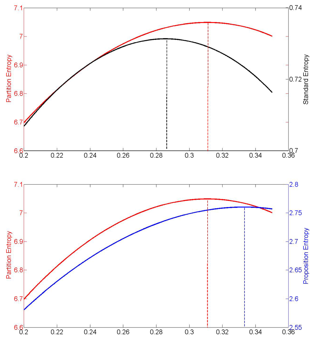
Figure 1. Plotted are the partition entropy, the standard entropy and the proposition entropy under the constraints, $P({\omega }_1)+P({\omega }_2)+P({\omega }_3)+P({\omega }_4)=1$, $P({\omega }_1)+2.75P({\omega }_2)+7.1P({\omega }_3)=1.7,P({\omega }_4)=0$, as a function of $P({\omega }_2).$ The dotted lines indicate the respective maxima, which obtain for different values of $P({\omega }_2).$

2.3. Loss

As Ramsey observed, all our lives, we are, in a sense, betting. The strengths of our beliefs guide our actions and expose us to possible losses. If we go to the station when the train happens not to run, we incur a loss: a wasted journey to the station and a delay in getting to where we want to go. Normally, when we are deliberating about how strongly to believe a proposition, we have no realistic idea as to the losses to which that belief will expose us. That is, when determining a belief function B, we do not know the true loss function, $L^{*}$.

Now, a loss function L is standardly defined as a function $L:\Omega \times \mathbb{P}⟶(-\infty ,\infty ]$, where $L(\omega ,P)$ is the loss one incurs by adopting probability function $P\in \mathbb{P}$ when ω is the true state of the world. Note that a standard loss function will only evaluate an agent’s beliefs about the states, not the extent to which she believes other propositions. This is appropriate when belief is assumed to be probabilistic, because a probability function is determined by its values on the states. But we are concerned with justifying the probability norm here and, hence, need to consider the full range of the agent’s beliefs, in order to show that they should satisfy the axioms of probability. Hence, we need to extend the concept of a loss function to evaluate all of the agent’s beliefs:

Definition 4 (Loss function). A loss function is a function $L:\mathcal{P}\Omega \times ⟨\mathbb{B}⟩⟶(-\infty ,\infty ]$.

$L(F,B)$ is the loss incurred by a belief function B, when proposition F turns out to be true. We shall interpret this loss as the loss that is attributable to F in isolation from all other propositions, rather than the total loss incurred when proposition F turns out to be true. When F turns out to be true, so does any proposition G, for $F\subset G$. Thus, the total loss when F turns out to be true includes $L(G,B)$, as well as $L(F,B)$. The total loss on F turning out to be true might therefore be represented by ${\sum }_{G\supseteq F}L(G,B)$, with $L(F,B)$ being the loss distinctive to F, i.e., the loss on F turning out to be true over and above the loss incurred by $G\supset F$.

Is there anything that one can presume about a loss function in the absence of any information about the true loss function, $L^{*}$? Plausibly:

L1. 

$L(F,B)=0$ if $B(F)=1$.

L2. 

$L(F,B)$ strictly increases as $B(F)$ decreases from one towards zero.

L3. 

$L(F,B)$ depends only on $B(F)$.

To express the next condition, we need some notation. Suppose $\mathcal{L}={\mathcal{L}}_1\cup {\mathcal{L}}_2$: say that $\mathcal{L}=\{A_1,...,A_n\}$, ${\mathcal{L}}_1=\{A_1,...,A_m\}$, ${\mathcal{L}}_2=\{A_{m+1},...,A_n\}$ for some $1<m<n$. Then, $\omega \in \Omega$ takes the form ${\omega }_1\wedge {\omega }_2$, where ${\omega }_1\in {\Omega }_1$ is a state of ${\mathcal{L}}_1$, and ${\omega }_2\in {\Omega }_2$ is a state of ${\mathcal{L}}_2$. Given propositions, $F_1\subseteq {\Omega }_1$ and $F_2\subseteq {\Omega }_2$, we can define $F_1\times F_2:=\{\omega ={\omega }_1\wedge {\omega }_2:{\omega }_1\in F_1,{\omega }_2\in F_2\}$, a proposition of $\mathcal{L}$. Given a fixed belief function, B, such that $B(\Omega )=1$, ${\mathcal{L}}_1$ and ${\mathcal{L}}_2$ are independent sublanguages, written ${\mathcal{L}}_1{⫫}_B{\mathcal{L}}_2$, if $B(F_1\times F_2)=B(F_1)·B(F_2)$ for all $F_1\subseteq {\Omega }_1$ and $F_2\subseteq {\Omega }_2$, where $B(F_1):=B(F_1\times {\Omega }_2)$ and $B(F_2):=B({\Omega }_1\times F_2)$. The restriction $B_{\downharpoonright {\mathcal{L}}_1}$ of B to ${\mathcal{L}}_1$ is a belief function on ${\mathcal{L}}_1$ defined by $B_{\downharpoonright {\mathcal{L}}_1}(F_1)=B(F_1)=B(F_1\times {\Omega }_2)$ and similarly for ${\mathcal{L}}_2$.

L4. 

Losses are additive when the language is composed of independent sublanguages: if $\mathcal{L}={\mathcal{L}}_1\cup {\mathcal{L}}_2$ for ${\mathcal{L}}_1{⫫}_B{\mathcal{L}}_2$, then $L(F_1\times F_2,B)=L_1(F_1,B_{\downharpoonright {\mathcal{L}}_1})+L_2(F_2,B_{\downharpoonright {\mathcal{L}}_2})$, where $L_1,L_2$ are loss functions defined on ${\mathcal{L}}_1,{\mathcal{L}}_2$, respectively.

L1 says that one should presume that fully believing a true proposition will not incur loss. L2 says that one should presume that the less one believes a true proposition, the more loss will result. L3 expresses the interpretation of $L(F,B)$ as the loss attributable to F in isolation of all other propositions. This condition, which is sometimes called locality, rules out that $L(F,B)$ depends on $B(F^{\prime })$ for $F^{\prime }\ne F$; it also rules out a dependence on $|F|$, for instance. L4 expresses the intuition that, at least if one supposes two propositions to be unrelated, one should presume that the loss on both turning out to be true is the sum of the losses on each. (These four conditions correspond to conditions L1–4 of pp. 64–65 in [1], which were put forward in the special case of loss functions defined over probability functions, as opposed to belief functions.)

The four conditions taken together tightly constrain the form of a presumed loss function, L:

Theorem 1. If loss functions are assumed to satisfy L1–4, then $L(F,B)=-klogB(F)$ for some constant, $k>0$, that does not depend on $\mathcal{L}$.

Proof: We shall first focus on a loss function, L, defined with respect to a language, $\mathcal{L}$, that contains at least two propositional variables.

L3 implies that $L(F,B)=f_{\mathcal{L}}(B(F))$, for some function, $f_{\mathcal{L}}:[0,1]⟶(-\infty ,\infty ]$.

For our fixed $\mathcal{L}$ and each $x,y\in [0,1]$, choose some particular $B\in ⟨\mathbb{B}⟩,{\mathcal{L}}_1,{\mathcal{L}}_2,F_1\subseteq {\Omega }_1,F_2\subseteq {\Omega }_2$, such that $\mathcal{L}={\mathcal{L}}_1\cup {\mathcal{L}}_2$, where ${\mathcal{L}}_1{⫫}_B{\mathcal{L}}_2$, $B(F_1)=x$ and $B(F_2)=y$. This is possible, because $\mathcal{L}$ has at least two propositional variables. Note in particular that since ${\mathcal{L}}_1$ and ${\mathcal{L}}_2$ are independent sublanguages, we have $B(\Omega )=1$.

Note that

$$1=B(\Omega )=B({\Omega }_1\times {\Omega }_2)=B_{\downharpoonright {\mathcal{L}}_1}({\Omega }_1)$$

(15)

and, similarly, $B_{\downharpoonright {\mathcal{L}}_2}({\Omega }_2)=1$. By L1, then, $L_1({\Omega }_1,B_{\downharpoonright {\mathcal{L}}_1})=L_2({\Omega }_2,B_{\downharpoonright {\mathcal{L}}_2})=0$.

Therefore, by applying L4 twice:

$$\begin{array}{ccc}\hfill f_{\mathcal{L}}(xy)& =& f_{\mathcal{L}}(B(F_1)·B(F_2))\hfill \\ & =& L(F_1\times F_2,B)\hfill \\ & =& L_1(F_1,B_{\downharpoonright {\mathcal{L}}_1})+L_2(F_2,B_{\downharpoonright {\mathcal{L}}_2})\hfill \\ & =& [L(F_1\times {\Omega }_2,B)-L_2({\Omega }_2,B_{\downharpoonright {\mathcal{L}}_2})]+[L({\Omega }_1\times F_2,B)-L_1({\Omega }_1,B_{\downharpoonright {\mathcal{L}}_1})]\hfill \\ & =& L(F_1\times {\Omega }_2,B)+L({\Omega }_1\times F_2,B)\hfill \\ & =& f_{\mathcal{L}}(x)+f_{\mathcal{L}}(y)\hfill \end{array}$$

(16)

The negative logarithm on $(0,1]$ is characterisable up to a multiplicative constant, $k_{\mathcal{L}}$, in terms of this additivity, together with the condition that $f_{\mathcal{L}}(x)\ge 0$, which is implied by L1–2 (see, e.g., Theorem 0.2.5 in [7]). L2 ensures that $f_{\mathcal{L}}$ is not zero everywhere, so $k_{\mathcal{L}}>0$.

We thus know that $f_{\mathcal{L}}(x)=-k_{\mathcal{L}}logx$ for $x\in (0,1].$ Now, note that for all $y\in (0,1]$, it needs to be the case that $f_{\mathcal{L}}(0)=f_{\mathcal{L}}(0·y)=f_{\mathcal{L}}(0)+f_{\mathcal{L}}(y)$, if $f_{\mathcal{L}}$ is to satisfy $f_{\mathcal{L}}(x·y)=f_{\mathcal{L}}(x)+f_{\mathcal{L}}(y)$ for all $x,y\in [0,1].$ Since $f_{\mathcal{L}}$ takes values in $(-\infty ,+\infty ]$, it follows that $f_{\mathcal{L}}(0)=+\infty .$

Thus far, we have shown that for a fixed language, $\mathcal{L}$, with at least two propositional variables, $L(F,B)=-k_{\mathcal{L}}logB(F)$ on $[0,1].$

Now consider an arbitrary language, ${\mathcal{L}}_1$, and a loss function $L_1$ on ${\mathcal{L}}_1$ which satisfies L1–L4. There exists some other language, ${\mathcal{L}}_2$, and a belief function B on $\mathcal{L}={\mathcal{L}}_1\cup {\mathcal{L}}_2$ such that ${\mathcal{L}}_1{⫫}_B{\mathcal{L}}_2.$ By the above, for the loss function L on $\mathcal{L}$, it holds that $L(F,B)=-k_{\mathcal{L}}logB(F)$ on $[0,1].$ By reasoning analogous to that above:

$$L_1(F_1,B_{\downharpoonright {\mathcal{L}}_1})=L(F_1\times {\Omega }_2,B)=f_{\mathcal{L}}(B(F_1\times {\Omega }_2))=f_{\mathcal{L}}(B_{\downharpoonright {\mathcal{L}}_1}(F_1))$$

(17)

Therefore, the loss function for ${\mathcal{L}}_1$ is $L_1(F_1,B_{\downharpoonright {\mathcal{L}}_1})=-k_{\mathcal{L}}log{B}_{\downharpoonright {\mathcal{L}}_1}(F_1).$ Thus, the constant $k_{\mathcal{L}}$ does not depend on the particular language $\mathcal{L}$ after all.

In general, then, $L(F,B)=-klogB(F)$ for some positive k.  ■

Since multiplication by a constant is equivalent to a change of base, we can take log to be the natural logarithm. Since we will be interested in the belief functions that minimise loss, rather than in the absolute value of any particular losses, we can take $k=1$ without loss of generality. Theorem 1 thus allows us to focus on the logarithmic loss function:

$$L^{log}(F,B):=-logB(F)$$

(18)

2.4. Score

In this paper, we are concerned with showing that the norms of objective Bayesianism must hold if an agent is to control her worst-case expected loss. Now, an expected loss function or scoring rule is standardly defined as $S_{\Omega }^L:\mathbb{P}\times \mathbb{P}⟶[-\infty ,\infty ]$ such that $S_{\Omega }^L(P,Q)={\sum }_{\omega \in \Omega }P(\omega )L_{\Omega }(\omega ,Q)$. This is interpretable as the expected loss incurred by adopting probability function Q as one’s belief function, when the probabilities are actually determined by P. (This is the statistical notion of a scoring rule as defined in [8]. More recently, a different, ‘epistemic’ notion of a scoring rule has been considered in the literature on non-pragmatic justifications of Bayesian norms; see, e.g., [9,10] and, also, a forthcoming paper by Landes, where similarities and differences of these two notions of a scoring rule are discussed. One difference that is significant to our purposes is that Predd et al.’s result in [11]—that for every epistemic scoring rule that is continuous and strictly proper, the set of non-dominated belief functions is the set $\mathbb{P}$ of probability functions—does not apply to statistical scoring rules. Furthermore, Predd et al. are only interested in justifying the probability norm by appealing to dominance as a decision theoretic norm. We are concerned with justifying three norms at once using worst-case loss avoidance as a desideratum. The epistemic approach is considered further in Section 5.4.)

While this standard definition of scoring rule is entirely appropriate when belief is assumed to be probabilistic, we make no such assumption here and need to consider scoring rules that evaluate all the agent’s beliefs, not just those concerning the states. In line with our discussion of entropy in Section 2.2, we shall consider the following generalisation:

Definition 5 (g-score). Given a loss function, L, and an inclusive weighting function, $g:\Pi ⟶{\mathbb{R}}_{\ge 0}$, the g-expected loss function or g-scoring rule or, simply, g-score is $S_g^L:\mathbb{P}\times ⟨\mathbb{B}⟩⟶[-\infty ,\infty ]$, such that

$$S_g^L(P,B)=\sum _{\pi \in \Pi }g(\pi )\sum _{F\in \pi }P(F)L(F,B)$$

(19)

Clearly, $S_{\Omega }^L$ corresponds to $S_{g_{\Omega }}^L$, where $g_{\Omega }$, which is not inclusive, is defined as in Section 2.2. We require that g be inclusive in Definition 5, since only in that case does the g-score genuinely evaluate all the agent’s beliefs. We will focus on $S_g^{log}(P^{*},B)$, i.e., the case in which the loss function is logarithmic and the expectation is taken with respect to the chance function, $P^{*}$, in order to show that an agent should satisfy the norms of objective Bayesianism if she is to control her worst-case g-expected logarithmic loss when her evidence determines that the chance function, $P^{*}$, is in $\mathbb{E}$.

For example, with the logarithmic loss function, the partition Π-score is defined by setting $g=g_{\Pi }$:

$$S_{\Pi }^{log}(P,B)=-\sum _{\pi \in \Pi }\sum _{F\in \pi }P(F)logB(F)$$

(20)

Similarly, the proposition $\mathcal{P}\Omega$-score is defined by setting $g=g_{\mathcal{P}\Omega }$:

$$S_{\mathcal{P}\Omega }^{log}(P,B)=-\sum _{F\subseteq \Omega }P(F)logB(F)$$

(21)

It turns out that the various logarithmic scoring rules have the following useful property:

Definition 6 (Strictly proper g-score). A scoring rule, $S_g^L:\mathbb{P}\times ⟨\mathbb{B}⟩⟶[-\infty ,\infty ]$, is strictly proper, if for all $P\in \mathbb{P}$, the function $S_g^L(P,·):⟨\mathbb{B}⟩⟶[-\infty ,\infty ]$ has a unique global minimum at $B=P$.

Definition 6 can be generalised: a scoring rule is strictly $\mathbb{X}$-proper if it is strictly proper for belief functions taken to be from a set $\mathbb{X}$. In Definition 6, $\mathbb{X}=⟨\mathbb{B}⟩$. The logarithmic scoring rule in the standard sense, i.e., ${\sum }_{\omega \in \Omega }P(\omega )L(\omega ,Q)$, is well known to be the only strictly $\mathbb{P}$-proper local scoring rule—see McCarthy [12] (p. 654), who credits Andrew Gleason for the uniqueness result; Shuford et al. [13] (p. 136) for the case of continuous scoring rules; Aczel and Pfanzagl [14] (Theorem 3, p. 101) for the case of differentiable scoring rules; and Savage [15] (§9.4). The logarithmic score in our sense, i.e., ${\sum }_{F\subseteq \Omega }P(F)L(F,B)$, is not strictly $\mathbb{Y}$-proper when $\mathbb{Y}$ is the set of non-normalised belief functions: $S(P,\mathit{bel})$ is a global minimum, where $\mathit{bel}$ is the belief function such that $\mathit{bel}(F)=1$ for all F. (While Joyce [9] (p. 276) suggests that logarithmic score is strictly $\mathbb{Y}$-proper for $\mathbb{Y}$ a set of non-normalised belief functions, he is referring to a logarithmic scoring rule that is different to the usual one considered above and that does not satisfy the locality condition, L3.)

On the way to showing that logarithmic g-scores are strictly proper, it will be useful to consider the following natural generalisation of Kullback-Leibler divergence to our framework:

Definition 7 (g-divergence). For a weighting function, $g:\Pi ⟶{\mathbb{R}}_{\ge 0}$, the g-divergence is the function, $d_g:\mathbb{P}\times ⟨\mathbb{B}⟩⟶[-\infty ,\infty ]$, defined by:

$$d_g(P,B)=\sum _{\pi \in \Pi }g(\pi )\sum _{F\in \pi }P(F)log\frac{P(F)}{B(F)}$$

(22)

Here, we adopt the usual convention that $0log\frac{0}{0}=0$ and $xlog\frac{x}{0}=+\infty$ for $x\in (0,1].$

We shall see that $d_g(P,B)$ is a sensible notion of the divergence of P from B by appealing to the following useful inequality (see, e.g., Theorem 2.7.1 in [16]):

Lemma 3 (Log sum inequality). For $x_i,y_i\in {\mathbb{R}}_{\ge 0},i,j=1,\dots ,k$,

$$(\sum _{i=1}^n{x}_i)log\frac{{\sum }_{i=1}^n{x}_i}{{\sum }_{i=1}^n{y}_i}\le \sum _{i=1}^n{x}_{i}log\frac{x_i}{y_i}$$

(23)

with equality, iff $x_i=c{y}_i$ for some constant, c, and $i=1,\dots ,k$.

Proposition 3. The following are equivalent:

• $d_g(P,B)\ge 0$ with equality iff $B=P$.
• g is inclusive.

Proof: First we shall see that if g is inclusive, then $d_g(P,B)\ge 0$ with equality iff $B=P$.

$$\begin{array}{ccc}\hfill d_g(P,B)& =& \sum _{\pi \in \Pi }g(\pi )\sum _{F\in \pi }P(F)log\frac{P(F)}{B(F)}\hfill \\ & \ge & \sum _{\pi \in \Pi }g(\pi )\left[\left(\sum _{F\in \pi }P(F)\right)log\frac{{\sum }_{F\in \pi }P(F)}{{\sum }_{F\in \pi }B(F)}\right]\hfill \\ & \ge & \sum _{\pi \in \Pi }g(\pi )\left[1log\frac{1}{1}\right]\hfill \\ & =& 0\hfill \end{array}$$

(24)

where the first inequality is an application of the log-sum inequality and the second inequality is a consequence of B being in $⟨\mathbb{B}⟩$. There is equality at the first inequality iff for all $F\subseteq \Omega$ and all π such that $F\in \pi$ and $g(\pi )>0$, $P(F^{\prime })=c_{\pi }B(F^{\prime })$ for all $F^{\prime }\in \pi$, and equality at the second inequality iff for all π such that $g(\pi )>0$, ${\sum }_{F\in \pi }B(F)=1$.

Clearly, if $B(F)=P(F)$ for all F, then these two equalities obtain. Conversely, suppose the two equalities obtain. Then, for each F, there is some $\pi =\{F=F_1,F_2,\dots ,F_k\}$ such that $g(\pi )>0$, because g is inclusive. The first equality condition implies that $P(F_i)=c_{\pi }B(F_i)$ for $i=1,\dots ,k$. The second equality implies that ${\sum }_{i=1}^{k}B(F_i)=1$. Hence, $1={\sum }_{i=1}^{k}P(F_i)=c_{\pi }{\sum }_{i=1}^{k}B(F_i)=c_{\pi }$, and so, $P(F_i)=B(F_i)$ for $i=1,\dots ,k$. In particular, $B(F)=P(F)$.

Next, we shall see that the condition that g is inclusive is essential.

If g were not inclusive, then there would be some $F\subseteq \Omega$ such that $g(\pi )=0$, for all $\pi \in \Pi$ such that $F\in \pi$. There are two cases.

(i)

$\varnothing \subset F\subset \Omega$. Take some $P\in \mathbb{P}$ such that $P(F)>0.$ Now, define $B(F):=0,$ and $B(F^{\prime }):=P(F^{\prime })$ for all other $F^{\prime }.$ Then, $B(\Omega )=1$ and ${\sum }_{G\in \pi }B(G)\le 1$ for all other $\pi \in \Pi$, so $B\in \mathbb{B}\subseteq ⟨\mathbb{B}⟩$. Furthermore, $d_g(P,P)=d_g(P,B)=0$.

(ii)

$F=\varnothing$ or $F=\Omega$. Define $B(\varnothing ):=B(\Omega ):=0.5$ and $B(F):=P(F)$ for all $\varnothing \subset F\subset \mathcal{P}\Omega .$ Then, $B(\varnothing )+B(\Omega )=1$ and ${\sum }_{G\in \pi }B(G)\le 1$ for all other $\pi \in \Pi$, so $B\in \mathbb{B}\subseteq ⟨\mathbb{B}⟩$. Furthermore, $d_g(P,P)=d_g(P,B)=0$.

In either case, then, $d_g(P,B)$ is not uniquely minimised by $B=P$.  ■

Corollary 3. The logarithmic g-score is strictly proper.

Proof: Recall that in the context of a g-score, g is inclusive.

$$\begin{array}{ccc}\hfill S_g^{log}(P,B)-S_g^{log}(P,P)& =& -\sum _{\pi \in \Pi }g(\pi )\sum _{F\in \pi }P(F)log\frac{B(F)}{P(F)}\hfill \\ & =& \sum _{\pi \in \Pi }g(\pi )\sum _{F\in \pi }P(F)log\frac{P(F)}{B(F)}\hfill \\ & =& d_g(P,B)\hfill \end{array}$$

(25)

Proposition 3 then implies that $S_g^{log}(P,B)-S_g^{log}(P,P)\ge 0$ with equality, iff $B=P$, i.e., $S_g^{log}$ is strictly proper.  ■

Finally, logarithmic g-scores are non-negative strictly convex functions in the following qualified sense:

Proposition 4. The logarithmic g-score $S_g^{log}(P,B)$ is non-negative and convex as a function of $B\in ⟨\mathbb{B}⟩$. Convexity is strict, i.e., $S_g^{log}(P,\lambda B_1+(1-\lambda )B_2)<\lambda S_g^{log}(P,B_1)+(1-\lambda )S_g^{log}(P,B_2)$ for $\lambda \in (0,1)$, unless $B_1$ and $B_2$ agree everywhere, except where $P(F)=0$.

Proof: The logarithmic g-score is non-negative, because $B(F),P(F)\in [0,1]$ for all F; so, $logB(F)\le 0$, $P(F)logB(F)\le 0$, and $g(\pi )>0$.

That $S_g^{log}(P,B)$ is strictly convex as a function of $⟨\mathbb{B}⟩$ follows from the strict concavity of $logx$. Take distinct $B_1,B_2\in ⟨\mathbb{B}⟩$ and $\lambda \in (0,1)$, and let $B=\lambda B_1+(1-\lambda )B_2$. Now:

$$\begin{array}{cc}\hfill P(F)logB(F)& =P(F)log(\lambda ·B_1(F)+(1-\lambda )B_2(F))\hfill \\ & \ge P(F)\left(\lambda log{B}_1(F)+(1-\lambda )log{B}_2(F)\right)\hfill \\ & =\lambda P(F)log{B}_1(F)+(1-\lambda )P(F)log{B}_2(F)\hfill \end{array}$$

(26)

with equality iff either $P(F)=0$ or $B_1(F)=B_2(F)$.

Hence:

$$\begin{array}{ccc}\hfill S_g^{log}(P,B)& =& -\sum _{\pi \in \Pi }g(\pi )\sum _{F\in \pi }P(F)logB(F)\hfill \\ & \le & \lambda S_g^{log}(P,B_1)+(1-\lambda )S_g^{log}(P,B_2)\hfill \end{array}$$

(27)

with equality iff $B_1$ and $B_2$ agree everywhere, except possibly where $P(F)=0$.  ■

2.5. Minimising the Worst-Case Logarithmic g-Score

In this section, we shall show that the g-entropy maximiser minimises the worst-case logarithmic g-score.

In order to prove our main result (Theorem 2), we would like to apply a game-theoretic minimax theorem, which will allow us to conclude that:

$$\underset{B\in \mathbb{B}}{inf}\underset{P\in \mathbb{E}}{sup}{S}_g^{log}(P,B)=\underset{P\in \mathbb{E}}{sup}\underset{B\in \mathbb{B}}{inf}{S}_g^{log}(P,B)$$

Note that the expression on the left-hand side describes the minimising worst-case g-score, where the worst case refers to P ranging in $\mathbb{E}.$ Speaking in game-theoretic lingo: the player playing first on the left-hand side aims to find the belief function(s) that minimises worst-case g-expected loss; again, the worst case is taken with respect to varying $P.$

For this approach to work, we would normally need $\mathbb{B}$ to be some set of mixed strategies. It is not obvious how $\mathbb{B}$ could be represented as a mixing of finitely many pure strategies. However, there exists a broad literature on minimax theorems [17], and we shall apply a theorem proven in König [18]. This theorem requires that certain level sets, in the set of functions in which the player aiming to minimise may chose his functions, are connected. To apply König’s result, we will thus allow the belief functions, B, to range in $⟨\mathbb{B}⟩,$ which has this property. It will follow that the $B\in ⟨\mathbb{B}⟩\setminus \mathbb{B}$ are never good choices for the minimising player playing first: the best choice is in $\mathbb{E}$, which is a subset of $\mathbb{B}.$

Having established that the inf and the sup commute, the rest is straightforward. Since the scoring rule we employ, $S_g^{log}$, is strictly proper, we have that the best strategy for the minimising player, answering a move by the maximising player, is to select the same function as the maximising player. Thus, it is best for the maximising player playing first to choose a/the function that maximises $S_g^{log}(P,P).$ We will thus find that:

$$\begin{array}{c}\hfill \underset{P\in \mathbb{E}}{sup}\underset{B\in ⟨\mathbb{B}⟩}{inf}{S}_g^{log}(P,B)=\underset{P\in \mathbb{E}}{sup}\underset{B\in \{P\}}{inf}{S}_g^{log}(P,B)=\underset{P\in \mathbb{E}}{sup}{S}_g^{log}(P,P)=\underset{P\in \mathbb{E}}{sup}{H}_g(P)\end{array}$$

Thus, worst-case g-expected loss and g-entropy have the same value. In game-theoretic terms: we find that our zero-sum g-log-loss game has a value. It remains to be shown that both players, when playing first, have a unique best choice, $P^{†}.$

First, then, we shall apply König’s result.

Definition 8 (König [18], p. 56). For $F:\mathbb{X}\times \mathbb{Y}\to [-\infty ,\infty ]$, we call $I\subset \mathbb{R}$ a border interval of F, if and only if I is an interval of the form $I=({sup}_{x\in \mathbb{X}}{inf}_{y\in \mathbb{Y}}F(x,y),+\infty ).$ $\Lambda \subset \mathbb{R}$ is called a border set of F if and only if $inf\Lambda ={sup}_{x\in \mathbb{X}}{inf}_{y\in \mathbb{Y}}F(x,y).$

For $\lambda \in \mathbb{R}$ and $\varnothing \subset K\subseteq \mathbb{Y}$, define $s_{\lambda }$ and ${\sigma }_{\lambda }$ to consist of $\mathbb{X}$ and of subsets of $\mathbb{X}$ of the form:

$$\bigcap _{y\in K}[F(·,y)>\lambda ]\text{respectively}\bigcap _{y\in K}[F(·,y)\ge \lambda ]$$

For $\lambda \in \mathbb{R}$ and finite $\varnothing \subset H\subseteq \mathbb{X}$, define $t_{\lambda }$ and ${\tau }_{\lambda }$ to consist of subsets of $\mathbb{Y}$ of the form:

$$\bigcap _{x\in H}[F(x,·)<\lambda ]\text{respectively}\bigcap _{x\in H}[F(x,·)\le \lambda ]$$

The following may be found in König [18] (Theorem 1.3, p. 57):

Lemma 4 (König’s Minimax). Let $\mathbb{X},\mathbb{Y}$ be topological spaces, $\mathbb{Y}$ be compact and Hausdorff and let $F:\mathbb{X}\times \mathbb{Y}\to [-\infty ,\infty ]$ be lower semicontinuous. Then, if Λ is some border set, I some border interval of F and if at least one of the following conditions holds:

• for all $\lambda \in \Lambda$, all members of $s_{\lambda }$ and ${\tau }_{\lambda }$ are connected;
• for all $\lambda \in \Lambda$, all members of $s_{\lambda }$ are connected and all $\lambda \in I$ all $t_{\lambda }$ are connected;
• for all $\lambda \in \Lambda$, all members of ${\sigma }_{\lambda }$ and $t_{\lambda }$ are connected;
• for all $\lambda \in \Lambda$, all members of ${\sigma }_{\lambda }$ are connected and all $\lambda \in I$ all ${\tau }_{\lambda }$ are connected;

then:

$$\underset{y\in \mathbb{Y}}{inf}\underset{x\in \mathbb{X}}{sup}F(x,y)=\underset{x\in \mathbb{X}}{sup}\underset{y\in \mathbb{Y}}{inf}F(x,y)$$

Lemma 5. $S_g^{log}:\mathbb{E}\times ⟨\mathbb{B}⟩\to [0,\infty ]$ is lower semicontinuous.

Proof: It suffices to show that $\{(P,B)\in \mathbb{E}\times ⟨\mathbb{B}⟩|S_g^{log}(P,B)\le r\}$ is closed for all $r\in \mathbb{R}.$ For $r\in \mathbb{R}$ consider a sequence ${(P_t,B_t)}_{t\in \mathbb{N}}$ with ${lim}_{t\to \infty }(P_t,B_t)=(P,B)$, such that $S_g^{log}(P_t,B_t)\le r$ for all t. Then:

$$\begin{array}{cc}\hfill S_g^{log}(P,B)& =-\sum _{\pi \in \Pi }g(\pi )\sum _{F\in \pi }P(F)logB(F)\hfill \\ & =\sum _{\pi \in \Pi }\sum _{\begin{array}{c}F\in \pi \\ g(\pi )P(F)>0\end{array}}-g(\pi )P(F)logB(F).\hfill \end{array}$$

(28)

If $g(\pi )P(F)>0$ and $B_t(F)$ converges to zero, then there is an $T\in \mathbb{N}$ such that for all $t\ge T$, $-g(\pi )P_t(F)log{B}_t(F)>r+1.$ Thus, $B_t(F)$ cannot converge to zero if $P(F)>0.$ Since $(B_t)$ converges, it has to converge to some $B(F)>0.$ Thus, when $g(\pi )P(F)>0$ we have that $-g(\pi )P(F)logB(F)={lim}_{t\to \infty }-g(\pi )P_t(F)log{B}_t(F)\le r.$ From $S_g^{log}(P_t,B_t)\le r$, we conclude that:

$$\begin{array}{cc}\hfill \sum _{\pi \in \Pi }\sum _{\begin{array}{c}F\in \pi \\ g(\pi )P(F)>0\end{array}}-g(\pi )P(F)logB(F)& =\underset{t\to \infty }{lim}\sum _{\pi \in \Pi }\sum _{\begin{array}{c}F\in \pi \\ g(\pi )P(F)>0\end{array}}-g(\pi )P_t(F)log{B}_t(F)\hfill \\ & \le r\hfill \end{array}$$

(29)

 ■

Proposition 5. For all $\mathbb{E}$:

$$\begin{array}{c}\hfill \underset{B\in ⟨\mathbb{B}⟩}{inf}\underset{P\in \mathbb{E}}{sup}{S}_g^{log}(P,B)=\underset{P\in \mathbb{E}}{sup}\underset{B\in ⟨\mathbb{B}⟩}{inf}{S}_g^{log}(P,B)\end{array}$$

Proof: It suffices to verify that the conditions of Lemma 4 are satisfied.

$\mathbb{E},⟨\mathbb{B}⟩$ are subsets of ${\mathbb{R}}^{|\Omega |}$, ${\mathbb{R}}^{|\mathcal{P}\Omega |}$ respectively, thus naturally equipped with the induced topology. $⟨\mathbb{B}⟩$ is compact and Hausdorff (see Lemma 1). $S_g^{log}:\mathbb{E}\times ⟨\mathbb{B}⟩\to [0,\infty ]$ is lower semicontinuous (see Lemma 5).

We need to show that one of the connectivity conditions holds. In fact, they all hold, as we shall see.

Note that $\mathbb{E},⟨\mathbb{B}⟩$ are connected, since they are convex.

For the $s_{\lambda }$ and ${\sigma }_{\lambda }$ consider any $B\in ⟨\mathbb{B}⟩$ and suppose that $P,P^{\prime }\in \mathbb{E}$ are such that $S_g^{log}(P,B)\stackrel{\ge }{>}\lambda$ and $S_g^{log}(P^{\prime },B)\stackrel{\ge }{>}\lambda .$ Then for $\eta \in (0,1)$ we have:

$$\begin{array}{cc}\hfill S_g^{log}(\eta P+(1-\eta )P^{\prime },B)& =-\sum _{\pi \in \Pi }g(\pi )\sum _{F\in \pi }(\eta P+(1-\eta )P^{\prime })(F)logB(F)\hfill \\ & =\eta S_g^{log}(P,B)+(1-\eta )S_g^{log}(P^{\prime },B)\hfill \\ & \stackrel{\ge }{>}\lambda \hfill \end{array}$$

(30)

Thus,

$$\begin{array}{c}\hfill \{P\in \mathbb{E}|S_g^{log}(P,B)\stackrel{\ge }{>}\lambda \}\end{array}$$

(31)

is convex for all $B\in ⟨\mathbb{B}⟩.$

Thus, every intersection of such sets is convex. Hence, these intersections are connected. (If any such intersection is empty, then it is trivially connected.)

For the $t_{\lambda }$ and ${\tau }_{\lambda }$, note that for every $P\in \mathbb{P}$, we have that

$$\begin{array}{c}\hfill \{B\in ⟨\mathbb{B}⟩|S_g^{log}(P,B)\stackrel{\le }{<}\lambda \}\end{array}$$

(32)

is convex, which follows from Proposition 4 by noting that for a convex function (here, $S_g^{log}(P,·)$) on a convex set (here, $⟨\mathbb{B}⟩$), the set of elements in the domain that are mapped to a number (strictly) less than λ is convex for all $\lambda \in \mathbb{R}.$

Thus, every intersection of such sets is convex. Hence, these intersections are connected.  ■

The suprema and infima referred to in Proposition 5 may not be achieved at points of $\mathbb{E}$. If not, they will be achieved instead at points in the closure, $\left[\mathbb{E}\right]$, of $\mathbb{E}$. We shall use $arg{sup}_{P\in \mathbb{E}}$ (and $arg{inf}_{P\in \mathbb{E}}$) to refer to the points in $\left[\mathbb{E}\right]$ that achieve the supremum (respectively, infimum), whether or not these points are in $\mathbb{E}$.

Theorem 2. As usual, $\mathbb{E}$ is taken to be convex and g inclusive. We have that:

$$\begin{array}{c}\hfill arg\underset{P\in \mathbb{E}}{sup}{H}_g(P)=arg\underset{B\in \mathbb{B}}{inf}\underset{P\in \mathbb{E}}{sup}{S}_g^{log}(P,B)\end{array}$$

(33)

Proof: We shall prove the following slightly stronger equality, allowing B to range in $⟨\mathbb{B}⟩$, instead of $\mathbb{B}$:

$$\begin{array}{c}\hfill arg\underset{P\in \mathbb{E}}{sup}{H}_g(P)=arg\underset{B\in ⟨\mathbb{B}⟩}{inf}\underset{P\in \mathbb{E}}{sup}{S}_g^{log}(P,B)\end{array}$$

(34)

The theorem then follows from the following fact. The right-hand side of Equation (34) is an optimization problem, where the optimum (here, we look for the infimum of ${sup}_{P\in \mathbb{E}}{S}_g^{log}(P,·)$) uniquely obtains for a certain value (here, $P^{†}$). Restricting the domain of the variables (here, from $⟨\mathbb{B}⟩$ to $\mathbb{B}$) in the optimization problem, to a subdomain that contains optimum $P^{†}\in \left[\mathbb{E}\right]\subseteq \mathbb{B}\subseteq ⟨\mathbb{B}⟩$, does not change where the optimum obtains nor the value of the optimum.

Note that:

$$\begin{array}{cc}\hfill \underset{P\in \mathbb{E}}{sup}{H}_g(P)& =\underset{P\in \mathbb{E}}{sup}{S}_g^{log}(P,P)\hfill \\ & \stackrel{}{=}\underset{P\in \mathbb{E}}{sup}\underset{B\in ⟨\mathbb{B}⟩}{inf}{S}_g^{log}(P,B)\hfill \\ & \stackrel{}{=}\underset{B\in ⟨\mathbb{B}⟩}{inf}\underset{P\in \mathbb{E}}{sup}{S}_g^{log}(P,B)\hfill \end{array}$$

(35)

The first equality is simply the definition of $H_g.$ The second equality follows directly from strict propriety (Corollary 3). To obtain the third line, we apply Proposition 5.

It remains to show that we can introduce arg on both sides of Equation (33).

The following sort of argument seems to be folklore in game theory; we here adapt (Lemma 4.1 on p. 1384 in [3]) for our purposes. We have:

$$\begin{array}{cc}\hfill P^{†}:& =arg\underset{P\in \mathbb{E}}{sup}{S}_g^{log}(P,P)\hfill \end{array}$$

(36)

$$\begin{array}{cc}& =arg\underset{P\in \mathbb{E}}{sup}\underset{B\in ⟨\mathbb{B}⟩}{inf}{S}_g^{log}(P,B)\hfill \end{array}$$

(37)

The $argsup$ in Equation (36) is unique (Corollary 2). Equation (37) follows from strict propriety of $S_g^{log}$ (Corollary 3). Now let:

$$\begin{array}{c}\hfill B^{†}\in arg\underset{B\in ⟨\mathbb{B}⟩}{inf}\underset{P\in \mathbb{E}}{sup}{S}_g^{log}(P,B)\end{array}$$

(38)

Then:

$$\begin{array}{cc}\hfill S_g^{log}(P^{†},P^{†})& =\underset{P\in \mathbb{E}}{sup}\underset{B\in ⟨\mathbb{B}⟩}{inf}{S}_g^{log}(P,B)\hfill \\ & =\underset{B\in ⟨\mathbb{B}⟩}{inf}{S}_g^{log}(P^{†},B)\hfill \\ & \le S_g^{log}(P^{†},B^{†})\hfill \\ & \le \underset{P\in \mathbb{E}}{sup}{S}_g^{log}(P,B^{†})\hfill \end{array}$$

(39)

$$\begin{array}{cc}& =\underset{B\in ⟨\mathbb{B}⟩}{inf}\underset{P\in \mathbb{E}}{sup}{S}_g^{log}(P,B)\hfill \end{array}$$

(40)

The first equality follows from the definition of $P^{†}$; see Equations (36) and (37). That we may drop the sup again follows from the definition of $P^{†},$ since $P^{†}$ maximises ${inf}_{B\in ⟨\mathbb{B}⟩}{S}_g^{log}(·,B).$ The inequalities hold, since dropping a minimisation and introducing a maximisation can only lead to an increase. The final inequality is immediate from the definition of $B^{†}$ minimising ${sup}_{P\in \mathbb{E}}{S}_g^{log}(P,·).$

By Proposition 5, all inequalities above are in fact equalities. From $S_g^{log}(P^{†},P^{†})=S_g^{log}(P^{†},B^{†})$ and strict propriety, we may now infer that $B^{†}=P^{†}.$  ■

In sum, then, if an agent is to minimise her worst-case g-score, then her belief function needs to be the probability function in $\mathbb{E}$ that maximises g-entropy, as long as this entropy maximiser is in $\mathbb{E}$. That the belief function is to be a probability function is the content of the probability norm; that it is to be in $\mathbb{E}$ is the content of the calibration norm; that it is to maximise g-entropy is related to the equivocation norm. We shall defer a full discussion of the equivocation norm to Section 4. In the next section, we shall show that the arguments of this section generalise to belief as defined over sentences rather than propositions. This will imply that logically equivalent sentences should be believed to the same extent—an important component of the probability norm in the sentential framework.

We shall conclude this section by providing a slight generalisation of the previous result. Note that, thus far, when considering worst-case g-score, this worst case is with respect to a chance function taken to be in $\mathbb{E}=⟨{\mathbb{P}}^{*}⟩$. However, the evidence determines something more precise, namely that the chance function is in ${\mathbb{P}}^{*}$, which is not assumed to be convex. The following result indicates that our main argument will carry over to this more precise setting.

Theorem 3. Suppose ${\mathbb{P}}^{*}\subseteq \mathbb{P}$ is such that the unique g-entropy maximiser, $P^{†}$, for $\left[\mathbb{E}\right]=\left[⟨{\mathbb{P}}^{*}⟩\right]$, is in $\left[{\mathbb{P}}^{*}\right]$. Then:

$$\begin{array}{c}\hfill P^{†}=arg\underset{P\in \mathbb{E}}{sup}{H}_g(P)=arg\underset{B\in \mathbb{B}}{inf}\underset{P\in {\mathbb{P}}^{*}}{sup}{S}_g^{log}(P,B)\end{array}$$

(41)

Proof: As in the previous proof, we shall prove a slightly stronger equality:

$$\begin{array}{c}\hfill P^{†}=arg\underset{P\in \mathbb{E}}{sup}{H}_g(P)=arg\underset{B\in ⟨\mathbb{B}⟩}{inf}\underset{P\in {\mathbb{P}}^{*}}{sup}{S}_g^{log}(P,B)\end{array}$$

(42)

The result follows for the same reasons given in the proof of Theorem 2.

From the strict propriety of $S_g^{log}$, we have:

$$\begin{array}{cc}\hfill S_g^{log}(P^{†},P^{†})& =\underset{B\in ⟨\mathbb{B}⟩}{inf}{S}_g^{log}(P^{†},B)\hfill \\ & \le \underset{B\in ⟨\mathbb{B}⟩}{inf}\underset{P\in {\mathbb{P}}^{*}}{sup}{S}_g^{log}(P,B)\hfill \\ & \le \underset{B\in ⟨\mathbb{B}⟩}{inf}\underset{P\in ⟨{\mathbb{P}}^{*}⟩}{sup}{S}_g^{log}(P,B)\hfill \\ & =\underset{P\in ⟨{\mathbb{P}}^{*}⟩}{sup}{S}_g^{log}(P,P^{†})\hfill \\ & =S_g^{log}(P^{†},P^{†})\hfill \end{array}$$

(43)

where the last two equalities are simply Theorem 2. Hence:

$$\begin{array}{c}\hfill \underset{B\in ⟨\mathbb{B}⟩}{inf}\underset{P\in {\mathbb{P}}^{*}}{sup}{S}_g^{log}(P,B)=S_g^{log}(P^{†},P^{†})=\underset{P\in \mathbb{E}}{sup}{H}_g(P)=\underset{P\in {\mathbb{P}}^{*}}{sup}{H}_g(P)\end{array}$$

That is, the lowest worst case expected loss is the same for $P\in \left[{\mathbb{P}}^{*}\right]$ and $P\in \left[⟨{\mathbb{P}}^{*}⟩\right].$

Furthermore, since $S_g^{log}(P^{†},P^{†})={sup}_{P\in \left[⟨{\mathbb{P}}^{*}⟩\right]}{S}_g^{log}(P,P^{†})$ and since $P^{†}\in \left[{\mathbb{P}}^{*}\right]$, we have $S_g^{log}(P^{†},P^{†})={sup}_{P\in {\mathbb{P}}^{*}}{S}_g^{log}(P,P^{†})$. Thus, $B=P^{†}$ minimises ${sup}_{P\in {\mathbb{P}}^{*}}{S}_g^{log}(P,B).$

Now, suppose that $B^{\prime }\in ⟨\mathbb{B}⟩$ is different from $P^{†}.$ Then:

$$\begin{array}{c}\hfill \underset{P\in {\mathbb{P}}^{*}}{sup}{S}_g^{log}(P,B^{\prime })\ge S_g^{log}(P^{†},B^{\prime })>S_g^{log}(P^{†},P^{†})\end{array}$$

(44)

where the strict inequality follows from strict propriety. This shows that adopting $B^{\prime }\ne P^{†}$ leads to an avoidably bad score.

Hence, $B=P^{†}$ is the unique function in $⟨\mathbb{B}⟩$ which minimises ${sup}_{P\in {\mathbb{P}}^{*}}{S}_g^{log}(P,B).$  ■

3. Belief over Sentences

Armed with our results for beliefs defined over propositions, we now tackle the case of beliefs defined over sentences, $S\mathcal{L}$, of a propositional language, $\mathcal{L}.$ The plan is as follows. First, we normalise the belief functions in Section 3.1. In Section 3.2, we motivate the use of logarithmic loss as a default loss function. We are able to define our logarithmic scoring rule in Section 3.3, and we show there that, with respect to our scoring rule, the generalised entropy maximiser is the unique belief function that minimises the worst-case expected loss.

Again, we shall not impose any restriction—such as additivity—on the agent’s belief function, now defined on the sentences of the propositional language $\mathcal{L}$. In particular, we do not assume that the agent’s belief function assigns logically equivalent sentences the same degree of belief. We shall show that any belief function violating this property incurs an avoidable loss. Thus, the results of this section allow us to show more than we could in the case of belief functions defined over propositions.

Several of the proofs in this section are analogous to the proofs of corresponding results presented in Section 2. They are included here in full for the sake of completeness; the reader may wish to skim over those details that are already familiar.

3.1. Normalisation

$S\mathcal{L}$ is the set of sentences of propositional language $\mathcal{L}$, formed as usual by recursively applying the connectives, $\neg ,\vee ,\wedge ,\to ,\leftrightarrow$, to the propositional variables, $A_1,\dots ,A_n$. A non-normalised belief function, $\mathit{bel}:S\mathcal{L}⟶{\mathbb{R}}_{\ge 0}$, is thus a function that maps any sentence of the language to a non-negative real number. As in Section 2.1, for technical convenience, we shall focus our attention on normalised belief functions.

Definition 9 (Representation). A sentence, $\theta \in S\mathcal{L}$, represents the proposition $F=\{\omega :\omega \vDash \theta \}$. Let $\mathcal{F}$ be a set of pairwise distinct propositions. We say that $\Theta \subseteq S\mathcal{L}$ is a set of representatives of $\mathcal{F},$ if and only if each sentence in Θ represents some proposition in $\mathcal{F}$ and each proposition in $\mathcal{F}$ is represented by a unique sentence in Θ. A set, ρ, of representatives of $\mathcal{P}\Omega$ will be called a representation. We denote by ϱ the set of all representations. For a set of pairwise distinct propositions, $\mathcal{F}$, and a representation, $\rho \in \varrho$, we denote by $\rho (\mathcal{F})\subset S\mathcal{L}$ the set of sentences in ρ that represent the propositions in $\mathcal{F}.$

We call ${\pi }_{\mathcal{L}}\subseteq S\mathcal{L}$ a partition of $S\mathcal{L},$ if and only if it is a set of representatives of some partition $\pi \in \Pi$ of propositions. We denote by ${\Pi }_{\mathcal{L}}$ the set of these ${\pi }_{\mathcal{L}}.$

Definition 10 (Normalised belief function on sentences). Define the set of normalized belief functions on $S\mathcal{L}$ as:

$$\begin{array}{c}\hfill {\mathbb{B}}_{\mathcal{L}}:=\{B_{\mathcal{L}}:S\mathcal{L}⟶[0,1]:\sum _{\phi \in {\pi }_{\mathcal{L}}}{B}_{\mathcal{L}}(\phi )\le 1\text{ for all }{\pi }_{\mathcal{L}}\in {\Pi }_{\mathcal{L}}\text{ and }\sum _{\phi \in {\pi }_{\mathcal{L}}}{B}_{\mathcal{L}}(\phi )=1\text{ for some }{\pi }_{\mathcal{L}}\in {\Pi }_{\mathcal{L}}\}\end{array}$$

The set of probability functions is defined as:

$$\begin{array}{c}\hfill {\mathbb{P}}_{\mathcal{L}}:=\{P_{\mathcal{L}}:S\mathcal{L}⟶[0,1]:\sum _{\phi \in {\pi }_{\mathcal{L}}}{P}_{\mathcal{L}}(\phi )=1\text{ for all }{\pi }_{\mathcal{L}}\in {\Pi }_{\mathcal{L}}\}\end{array}$$

As in the proposition case, we have:

Proposition 6. $P_{\mathcal{L}}\in {\mathbb{P}}_{\mathcal{L}}$ iff $P_{\mathcal{L}}:S\mathcal{L}⟶[0,1]$ satisfies the axioms of probability:

P1:

$P_{\mathcal{L}}(\tau )=1$ for all tautologies $\tau .$

P2:

If $\vDash \neg (\phi \wedge \psi )$ then $P_{\mathcal{L}}(\phi \vee \psi )=P_{\mathcal{L}}(\phi )+P_{\mathcal{L}}(\psi )$.

Proof: Suppose $P_{\mathcal{L}}\in {\mathbb{P}}_{\mathcal{L}}$. For any tautology, $\tau \in S\mathcal{L}$, it holds that $P_{\mathcal{L}}(\tau )=1$, because $\{\tau \}$ is a partition in ${\Pi }_{\mathcal{L}}.$ $P_{\mathcal{L}}(\neg \tau )=0$, because $\{\tau ,\neg \tau \}$ is a partition in ${\Pi }_{\mathcal{L}}$ and $P_{\mathcal{L}}(\tau )=1$.

Suppose that $\phi ,\psi \in S\mathcal{L}$ are such that $\vDash \neg (\phi \wedge \psi )$. We shall proceed by cases to show that $P_{\mathcal{L}}(\phi \vee \psi )=P_{\mathcal{L}}(\phi )+P_{\mathcal{L}}(\psi )$. In the first three cases, one of the sentences is a contradiction, in the last two cases, there are no contradictions.

(i)

$\vDash \phi$ and $\vDash \neg \psi ,$ then $\vDash \phi \vee \psi .$ Thus, by the above $P_{\mathcal{L}}(\phi )=1$ and $P_{\mathcal{L}}(\psi )=0$, and hence, $P_{\mathcal{L}}(\phi \vee \psi )=1=P_{\mathcal{L}}(\phi )+P_{\mathcal{L}}(\psi ).$

(ii)

$\vDash \neg \phi$ and $\vDash \neg \psi ,$ then $\vDash \neg \phi \vee \neg \psi .$ Thus, $P_{\mathcal{L}}(\phi \vee \psi )=0=P_{\mathcal{L}}(\phi )+P_{\mathcal{L}}(\psi ).$

(iii)

$⊭\neg \phi ,$ $⊭\phi ,$ and $\vDash \neg \psi ,$ then $\{\phi \vee \psi ,\neg \phi \vee \psi \}$ and $\{\phi ,\neg \phi \vee \psi \}$ are both partitions in ${\Pi }_{\mathcal{L}}.$ Thus, $P_{\mathcal{L}}(\phi \vee \psi )+P_{\mathcal{L}}(\neg \phi \vee \psi )=1=P_{\mathcal{L}}(\phi )+P_{\mathcal{L}}(\neg \phi \vee \psi ).$ Putting these observations together, we now find $P_{\mathcal{L}}(\phi \vee \psi )=P_{\mathcal{L}}(\phi )=P_{\mathcal{L}}(\phi )+P_{\mathcal{L}}(\psi ).$

(iv)

$⊭\neg \phi ,$ $⊭\neg \psi$ and $\vDash \phi \leftrightarrow \neg \psi ,$ then $\{\phi ,\psi \}$ is a partition and $\phi \vee \psi$ is a tautology. Hence, $P_{\mathcal{L}}(\phi )+P_{\mathcal{L}}(\psi )=1$ and $P_{\mathcal{L}}(\phi \vee \psi )=1$. This now yields $P_{\mathcal{L}}(\phi )+P_{\mathcal{L}}(\psi )=P_{\mathcal{L}}(\phi \vee \psi )$.

(v)

$⊭\neg \phi ,$ $⊭\neg \psi$ and $⊭\phi \leftrightarrow \neg \psi ,$ then none of the following sentences is a tautology or a contradiction: $\phi ,\psi ,\phi \vee \psi ,\neg (\phi \vee \psi ).$ Since $\{\phi ,\psi ,\neg (\phi \vee \psi )\}$ and $\{\phi \vee \psi ,\neg (\phi \vee \psi )\}$ are both partitions in ${\Pi }_{\mathcal{L}}$, we obtain $P_{\mathcal{L}}(\phi )+P_{\mathcal{L}}(\psi )=1-P_{\mathcal{L}}(\neg (\phi \vee \psi ))=P_{\mathcal{L}}(\phi \vee \psi )$. So, $P_{\mathcal{L}}(\phi )+P_{\mathcal{L}}(\psi )=P_{\mathcal{L}}(\phi \vee \psi )$.

On the other hand, suppose P1 and P2 hold. That ${\sum }_{\phi \in {\pi }_{\mathcal{L}}}{P}_{\mathcal{L}}(\phi )=1$ holds for all ${\pi }_{\mathcal{L}}\in {\Pi }_{\mathcal{L}}$ can be seen by induction on the size of ${\pi }_{\mathcal{L}}$. If $|{\pi }_{\mathcal{L}}|=1$, then $\pi =\{\tau \}$ for some tautology $\tau \in S\mathcal{L}$, and $P_{\mathcal{L}}(\tau )=1$ by P1. Suppose then that ${\pi }_{\mathcal{L}}=\{{\phi }_1,\dots ,{\phi }_{k+1}\}$ for $k\ge 1$. Now, ${\sum }_{i=1}^{k-1}{P}_{\mathcal{L}}({\phi }_i)+P_{\mathcal{L}}({\phi }_k\vee {\phi }_{k+1})=1$ by the induction hypothesis. Furthermore, $P_{\mathcal{L}}({\phi }_k\vee {\phi }_{k+1})=P_{\mathcal{L}}({\phi }_k)+P_{\mathcal{L}}({\phi }_{k+1})$ by P2, so ${\sum }_{\phi \in {\pi }_{\mathcal{L}}}{P}_{\mathcal{L}}(\phi )=1$, as required.  ■

Definition 11 (Respects logical equivalence). We say that a belief function $B_{\mathcal{L}}\in ⟨{\mathbb{B}}_{\mathcal{L}}⟩$ respects logical equivalence if and only if $\vDash \phi \leftrightarrow \psi$ implies $B_{\mathcal{L}}(\phi )=B_{\mathcal{L}}(\psi ).$

Proposition 7. The probability functions $P_{\mathcal{L}}\in {\mathbb{P}}_{\mathcal{L}}$ respect logical equivalence.

Proof: Suppose $P_{\mathcal{L}}\in {\mathbb{P}}_{\mathcal{L}}$ and assume that $\phi ,\psi \in S\mathcal{L}$ are logically equivalent. Note that $\psi \wedge \neg \phi \vDash A_1\wedge \neg A_1,$ $\psi \vee \neg \phi \vDash A_1\vee \neg A_1$ and that $\{\phi ,\neg \phi \}$ and $\{\psi ,\neg \phi \}$ are partitions in ${\Pi }_{\mathcal{L}}.$ Hence:

$$\begin{array}{c}\hfill P_{\mathcal{L}}(\phi )+P_{\mathcal{L}}(\neg \phi )=1=P_{\mathcal{L}}(\psi )+P_{\mathcal{L}}(\neg \phi )\end{array}$$

(45)

Therefore, $P_{\mathcal{L}}(\phi )=P_{\mathcal{L}}(\psi ).$

Thus, the $P_{\mathcal{L}}\in {\mathbb{P}}_{\mathcal{L}}$ assign logically equivalent formulae the same probability.  ■

3.2. Loss

By analogy with the line of argument of Section 2.3, we shall suppose that a default loss function, $L:S\mathcal{L}\times ⟨{\mathbb{B}}_{\mathcal{L}}⟩\to (-\infty ,\infty ]$, satisfies the following requirements:

L1. 

$L(\phi ,B_{\mathcal{L}})=0,$ if $B_{\mathcal{L}}(\phi )=1.$

L2. 

$L(\phi ,B_{\mathcal{L}})$ strictly increases as $B_{\mathcal{L}}(\phi )$ decreases from one towards zero.

L3. 

$L(\phi ,B_{\mathcal{L}})$ only depends on $B_{\mathcal{L}}(\phi )$.

Suppose we have a fixed belief function, $B_{\mathcal{L}}\in ⟨{\mathbb{B}}_{\mathcal{L}}⟩$, such that $B_{\mathcal{L}}(\tau )=1$ for any tautology, τ, and $\mathcal{L}={\mathcal{L}}_1\cup {\mathcal{L}}_2$, where ${\mathcal{L}}_1$ and ${\mathcal{L}}_2$ are independent sublanguages, written ${\mathcal{L}}_1{⫫}_{B_{\mathcal{L}}}{\mathcal{L}}_2$, i.e., $B_{\mathcal{L}}({\varphi }_1\wedge {\varphi }_2)=B_{\mathcal{L}}({\varphi }_1)·B_{\mathcal{L}}({\varphi }_2)$ for all ${\varphi }_1\in S{\mathcal{L}}_1$ and ${\varphi }_2\in S{\mathcal{L}}_2$. Let $B_{\downharpoonright {\mathcal{L}}_1}({\varphi }_1):=B_{\mathcal{L}}({\varphi }_1)$, $B_{\downharpoonright {\mathcal{L}}_2}({\varphi }_2):=B_{\mathcal{L}}({\varphi }_2)$.

L4. 

Losses are additive when the language is composed of independent sublanguages: if $\mathcal{L}={\mathcal{L}}_1\cup {\mathcal{L}}_2$ for ${\mathcal{L}}_1{⫫}_{B_{\mathcal{L}}}{\mathcal{L}}_2$, then $L({\varphi }_1\wedge {\varphi }_2,B_{\mathcal{L}})=L_1({\varphi }_1,B_{\downharpoonright {\mathcal{L}}_1})+L_2({\varphi }_2,B_{\downharpoonright {\mathcal{L}}_2})$, where $L_1,L_2$ are loss functions defined on ${\mathcal{L}}_1,{\mathcal{L}}_2$, respectively.

Theorem 4. If a loss function, L, on $S\mathcal{L}\times ⟨{\mathbb{B}}_{\mathcal{L}}⟩$ satisfies L1–4, then $L(\phi ,B_{\mathcal{L}})=-klog{B}_{\mathcal{L}}(\phi )$, where the constant, $k>0$, does not depend on the language, $\mathcal{L}$.

Proof: We shall first focus on a loss function, L, defined with respect to a language, $\mathcal{L}$, that contains at least two propositional variables.

L3 implies that $L(\phi ,B_{\mathcal{L}})=f_{\mathcal{L}}(B_{\mathcal{L}}(\phi ))$ for some function, $f_{\mathcal{L}}:[0,1]⟶(-\infty ,\infty ]$. For our fixed $\mathcal{L}$ and all $x,y\in [0,1]$, choose some $B_{\mathcal{L}}\in ⟨{\mathbb{B}}_{\mathcal{L}}⟩$ such that $\mathcal{L}={\mathcal{L}}_1\cup {\mathcal{L}}_2$, ${\mathcal{L}}_1{⫫}_{B_{\mathcal{L}}},{\mathcal{L}}_2$$B_{\mathcal{L}}({\varphi }_1)=x$, and $B_{\mathcal{L}}({\varphi }_2)=y$ for some ${\varphi }_1\in S{\mathcal{L}}_1,{\varphi }_2\in S{\mathcal{L}}_2.$ This is possible, because $\mathcal{L}$ contains at least two propositional variables.

Note that since ${\mathcal{L}}_1$ and ${\mathcal{L}}_2$ are independent sublanguages, given some specific tautology, ${\tau }_1$, of ${\mathcal{L}}_1$:

$$1=B_{\mathcal{L}}({\tau }_1)=B_{\downharpoonright {\mathcal{L}}_1}({\tau }_1)$$

(46)

$B_{\mathcal{L}}({\tau }_1)$ is well defined, since ${\tau }_1$ is a tautology of $S{\mathcal{L}}_1$, and every sentence in $S{\mathcal{L}}_1$ is a sentence in $S\mathcal{L}$. Similarly, $B_{\downharpoonright {\mathcal{L}}_2}({\tau }_2)=1$ for some specific tautology ${\tau }_2$ of ${\mathcal{L}}_2$. By L1, then, $L_1({\tau }_1,B_{\downharpoonright {\mathcal{L}}_1})=L_2({\tau }_2,B_{\downharpoonright {\mathcal{L}}_2})=0,$ where $L_1,$ respectively, $L_2,$ are the loss functions with respect to $S{\mathcal{L}}_1$ and $S{\mathcal{L}}_2$ satisfying L1–4. Thus:

$$\begin{array}{ccc}\hfill f_{\mathcal{L}}(x·y)& \stackrel{}{=}& f_{\mathcal{L}}(B_{\mathcal{L}}({\varphi }_1)·B_{\mathcal{L}}({\varphi }_2))\hfill \\ & \stackrel{L_3}{=}& L({\varphi }_1\wedge {\varphi }_2,B_{\mathcal{L}})\hfill \\ & \stackrel{L4}{=}& L_1({\varphi }_1,B_{\downharpoonright {\mathcal{L}}_1})+L_2({\varphi }_2,B_{\downharpoonright {\mathcal{L}}_2})\hfill \\ & \stackrel{L4}{=}& [L({\varphi }_1\wedge {\tau }_2,B_{\mathcal{L}})-L_2({\tau }_2,B_{\downharpoonright {\mathcal{L}}_2})]\hfill \\ & & +[L({\tau }_1\wedge {\varphi }_2,B_{\mathcal{L}})-L_1({\tau }_1,B_{\downharpoonright {\mathcal{L}}_1})]\hfill \\ & \stackrel{L1}{=}& L({\varphi }_1\wedge {\tau }_2,B_{\mathcal{L}})+L({\tau }_1\wedge {\varphi }_2,B_{\mathcal{L}})\hfill \\ & \stackrel{L3}{=}& f_{\mathcal{L}}(B_{\mathcal{L}}({\varphi }_1\wedge {\tau }_2))+f_{\mathcal{L}}(B_{\mathcal{L}}({\varphi }_2\wedge {\tau }_1))\hfill \\ & \stackrel{}{=}& f_{\mathcal{L}}(B_{\downharpoonright {\mathcal{L}}_1}({\varphi }_1)·B_{\downharpoonright {\mathcal{L}}_2}({\tau }_2))+f_{\mathcal{L}}(B_{\downharpoonright {\mathcal{L}}_1}({\tau }_1)·B_{\downharpoonright {\mathcal{L}}_2}({\varphi }_2))\hfill \\ & \stackrel{(46)}{=}& f_{\mathcal{L}}(B_{\downharpoonright {\mathcal{L}}_1}({\varphi }_1))+f_{\mathcal{L}}(B_{\downharpoonright {\mathcal{L}}_2}({\varphi }_2))\hfill \\ & \stackrel{}{=}& f_{\mathcal{L}}(B_{\mathcal{L}}({\varphi }_1))+f_{\mathcal{L}}(B_{\mathcal{L}}({\varphi }_2))\hfill \\ & \stackrel{}{=}& f_{\mathcal{L}}(x)+f_{\mathcal{L}}(y)\hfill \end{array}$$

(47)

The negative logarithm on $(0,1]$ is characterisable up to a multiplicative constant, $k_{\mathcal{L}}$, in terms of this additivity, together with the condition that $f_{\mathcal{L}}(x)\ge 0$, which is implied by L1–2 (see, e.g., Theorem 0.2.5 in [7]). L2 ensures that $f_{\mathcal{L}}$ is not zero everywhere, so $k_{\mathcal{L}}>0$. As in the corresponding proof for propositions, it follows that $f_{\mathcal{L}}(0)=+\infty .$

Thus far, we have shown that for a fixed language, $\mathcal{L}$, with at least two propositional variables, $L(F,B_{\mathcal{L}})=-k_{\mathcal{L}}log{B}_{\mathcal{L}}(F)$ on $[0,1].$

Now, focus on an arbitrary language, ${\mathcal{L}}_1$, and a corresponding loss function, $L_1$. We can choose ${\mathcal{L}}_2,\mathcal{L},B_{\mathcal{L}}$ such that $\mathcal{L}$ is composed of independent sublanguages, ${\mathcal{L}}_1$ and ${\mathcal{L}}_2.$ By reasoning analogous to that above:

$$\begin{array}{ccc}\hfill f_{{\mathcal{L}}_1}(B_{\downharpoonright {\mathcal{L}}_1}({\varphi }_1))& =& L_1({\varphi }_1,B_{\downharpoonright {\mathcal{L}}_1})\hfill \\ & =& L({\varphi }_1\wedge {\tau }_2,B_{\mathcal{L}})\hfill \\ & =& f_{\mathcal{L}}(B_{\mathcal{L}}({\varphi }_1\wedge {\tau }_2))\hfill \\ & =& f_{\mathcal{L}}(B_{\mathcal{L}}({\varphi }_1)·1)\hfill \\ & =& -k_{\mathcal{L}}log{B}_{\downharpoonright {\mathcal{L}}_1}({\varphi }_1)\hfill \end{array}$$

(48)

Therefore, the loss function for ${\mathcal{L}}_1$ is $L_1({\varphi }_1,B_{\downharpoonright {\mathcal{L}}_1})=-k_{\mathcal{L}}log{B}_{\downharpoonright {\mathcal{L}}_1}({\varphi }_1).$ Thus, the constant, $k_{\mathcal{L}}$, does not depend on $\mathcal{L}$ after all.

In general, then, $L(F,B_{\mathcal{L}})=-klog{B}_{\mathcal{L}}(F)$ for some positive k.  ■

Since multiplication by a constant is equivalent to a change of base, we can take log to be the natural logarithm. Since we will be interested in the belief functions that minimise loss, rather than in the absolute value of any particular losses, we can take $k=1$ without loss of generality. Theorem 4 thus allows us to focus on the logarithmic loss function:

$$L^{log}(F,B_{\mathcal{L}}):=-log{B}_{\mathcal{L}}(F)$$

(49)

3.3. Score, Entropy and Their Connection

In the case of belief over sentences, the expected loss varies according to which sentences are used to represent the various partitions of propositions. We can define the g-score to be the worst-case expected loss, where this worst case is taken over all possible representations:

Definition 12 (g-score). Given a loss function, $L,$ an inclusive weighting function, $g:\Pi ⟶{\mathbb{R}}_{\ge 0}$, and a representation, $\rho \in \varrho$, we define the representation-relative g-score $S_{g,\rho }^L:{\mathbb{P}}_{\mathcal{L}}\times ⟨{\mathbb{B}}_{\mathcal{L}}⟩⟶[-\infty ,\infty ]$ by

$$S_{g,\rho }^L(P_{\mathcal{L}},B_{\mathcal{L}}):=\sum _{\pi \in \Pi }g(\pi )\sum _{\phi \in \rho (\pi )}{P}_{\mathcal{L}}(\phi )L(\phi ,B_{\mathcal{L}})$$

(50)

and the (representation-independent) g-score $S_{g,\mathcal{L}}^L:{\mathbb{P}}_{\mathcal{L}}\times ⟨{\mathbb{B}}_{\mathcal{L}}⟩⟶[-\infty ,\infty ]$ by

$$S_{g,\mathcal{L}}^L(P_{\mathcal{L}},B_{\mathcal{L}}):=\underset{\rho \in \varrho }{sup}{S}_{g,\rho }^L(P_{\mathcal{L}},B_{\mathcal{L}})$$

(51)

In particular, for the logarithmic loss function under consideration here, we have:

$$S_{g,\rho }^{log}(P_{\mathcal{L}},B_{\mathcal{L}}):=-\sum _{\pi \in \Pi }g(\pi )\sum _{\phi \in \rho (\pi )}{P}_{\mathcal{L}}(\phi )log{B}_{\mathcal{L}}(\phi )$$

(52)

and:

$$S_{g,\mathcal{L}}^{log}(P_{\mathcal{L}},B_{\mathcal{L}}):=\underset{\rho \in \varrho }{sup}{S}_{g,\rho }^{log}(P_{\mathcal{L}},B_{\mathcal{L}})$$

(53)

We can thus define the g-entropy of a belief function on $S\mathcal{L}$ as:

$$\begin{array}{c}\hfill H_{g,\mathcal{L}}(B_{\mathcal{L}}):=S_{g,\mathcal{L}}^{log}(B_{\mathcal{L}},B_{\mathcal{L}})\end{array}$$

(54)

There is a canonical one-to-one correspondence between the $B_{\mathcal{L}}\in ⟨{\mathbb{B}}_{\mathcal{L}}⟩$ which respect logical equivalence and the $B\in ⟨\mathbb{B}⟩.$ In particular, ${\mathbb{P}}_{\mathcal{L}}$ can be identified with $\mathbb{P}.$ Moreover, any convex $\mathbb{E}\subseteq \mathbb{P}$ is in one-to-one correspondence with a convex ${\mathbb{E}}_{\mathcal{L}}\subseteq {\mathbb{P}}_{\mathcal{L}}.$ In the following, we shall make frequent use of this correspondence. For a $B_{\mathcal{L}}\in ⟨{\mathbb{B}}_{\mathcal{L}}⟩$ which respects logical equivalence, we denote by B the function in $⟨\mathbb{B}⟩$ with which it stands in one-to-one correspondence.

Lemma 6. If $B_{\mathcal{L}}\in ⟨{\mathbb{B}}_{\mathcal{L}}⟩$ respects logical equivalence, then for all $\rho \in \varrho$, we have $S_{g,\mathcal{L}}^{log}(P_{\mathcal{L}},B_{\mathcal{L}})={sup}_{\rho \in \varrho }{S}_{g,\rho }^{log}(P_{\mathcal{L}},B_{\mathcal{L}})=S_g^{log}(P,B).$

Proof: Simply note that $S_{g,\rho }^{log}(P_{\mathcal{L}},B_{\mathcal{L}})$ does not depend on $\rho .$  ■

Lemma 7. For all convex ${\mathbb{E}}_{\mathcal{L}}\subseteq {\mathbb{P}}_{\mathcal{L}}$:

$$\begin{array}{c}\hfill B_{\mathcal{L}}^{†}\in arg\underset{B_{\mathcal{L}}\in ⟨{\mathbb{B}}_{\mathcal{L}}⟩}{inf}\underset{P_{\mathcal{L}}\in {\mathbb{E}}_{\mathcal{L}}}{sup}\underset{\rho \in \varrho }{sup}{S}_{g,\rho }^{log}(P_{\mathcal{L}},B_{\mathcal{L}})\end{array}$$

respects logical equivalence.

Proof: Suppose that:

$$\begin{array}{c}\hfill B_{\mathcal{L}}^{†}\in arg\underset{B_{\mathcal{L}}\in ⟨{\mathbb{B}}_{\mathcal{L}}⟩}{inf}\underset{P_{\mathcal{L}}\in {\mathbb{E}}_{\mathcal{L}}}{sup}\underset{\rho \in \varrho }{sup}{S}_{g,\rho }^{log}(P_{\mathcal{L}},B_{\mathcal{L}})\end{array}$$

(55)

and assume that $B_{\mathcal{L}}^{†}$ does not respect logical equivalence. Then, define:

$$\begin{array}{c}\hfill B_{\mathcal{L}}^{inf}(\phi ):=\underset{\begin{array}{c}\theta \in S\mathcal{L}\\ \vDash \theta \leftrightarrow \phi \end{array}}{inf}{B}_{\mathcal{L}}^{†}(\theta )\end{array}$$

(56)

Since $B_{\mathcal{L}}^{†}$ does not respect logical equivalence, there are logically equivalent $\phi ,\psi$ such that $B_{\mathcal{L}}^{†}(\phi )\ne B_{\mathcal{L}}^{†}(\psi ).$ Hence, $B_{\mathcal{L}}^{inf}(\phi )<max\{B_{\mathcal{L}}^{†}(\phi ),B_{\mathcal{L}}^{†}(\psi )\}.$ Thus, for every ${\pi }_{\mathcal{L}}\in {\Pi }_{\mathcal{L}}$ with $\phi \in {\pi }_{\mathcal{L}}$, we have ${\sum }_{\chi \in {\pi }_{\mathcal{L}}}{B}_{\mathcal{L}}^{inf}(\chi )<1.$ Thus, $B_{\mathcal{L}}^{inf}\notin {\mathbb{P}}_{\mathcal{L}}.$ $B_{\mathcal{L}}^{inf}$ respects logical equivalence by definition.

Now, consider the function $B^{inf}:\mathcal{P}\Omega ⟶[0,1]$ which is determined by $B_{\mathcal{L}}^{inf}.$ Clearly, $B^{inf}\notin \mathbb{P}.$ There are two cases to consider.

(a) $B^{inf}\in ⟨\mathbb{B}⟩\setminus \mathbb{P}.$ Since $B^{inf}\notin \mathbb{P}$, by Theorem 2, we have that:

$$\begin{array}{c}\hfill \underset{P\in \mathbb{E}}{sup}{S}_g^{log}(P,B^{inf})>\underset{B\in ⟨\mathbb{B}⟩}{inf}\underset{P\in \mathbb{E}}{sup}{S}_g^{log}(P,B)\end{array}$$

(57)

(b) $B^{inf}\notin ⟨\mathbb{B}⟩$. Then, define $B^{\prime }$ by $B^{\prime }(F):=B^{inf}(F)+\delta$ for all $F\subseteq \Omega$, where $\delta \in (0,1]$ is minimal such that $B^{\prime }\in ⟨\mathbb{B}⟩.$ In particular, $B^{\prime }(\varnothing )\ge \delta >0,$ thus $B^{\prime }\notin \mathbb{P}.$ Moreover, whenever $P(F)>0$, it holds that $-P(F)log{B}^{inf}(F)>-P(F)log{B}^{\prime }(F)<+\infty .$ For the remainder of this proof, we shall extend the definition of the logarithmic g-score $S_g^{log}(P,B)$ by allowing the belief function, B, to be any non-negative function defined on $\mathcal{P}\Omega ,$ rather than just $B\in ⟨\mathbb{B}⟩$—if $B\notin ⟨\mathbb{B}⟩$, we shall be careful not to appeal to results that assume $B\in ⟨\mathbb{B}⟩$. We thus find for all $P\in \mathbb{P}$ that $S_g^{log}(P,B^{inf})>S_g^{log}(P,B^{\prime })<+\infty .$ Thus, by Theorem 2, we obtain the sharp inequality in the following:

$$\begin{array}{cc}\hfill \underset{P\in \mathbb{E}}{sup}{S}_g^{log}(P,B^{inf})& \ge \underset{P\in \mathbb{E}}{sup}{S}_g^{log}(P,B^{\prime })\hfill \\ & >\underset{B\in ⟨\mathbb{B}⟩}{inf}\underset{P\in \mathbb{E}}{sup}{S}_g^{log}(P,B)\hfill \end{array}$$

(58)

For both cases, we will obtain a contradiction:

$$\begin{array}{cc}\hfill S_g^{log}(P^{†},P^{†})& =\underset{P\in \mathbb{E}}{sup}{S}_g^{log}(P,P^{†})\hfill \end{array}$$

(59)

$$\begin{array}{cc}& =\underset{P_{\mathcal{L}}\in {\mathbb{E}}_{\mathcal{L}}}{sup}\underset{\rho \in \varrho }{sup}{S}_{g,\rho }^{log}(P_{\mathcal{L}},P_{\mathcal{L}}^{†})\hfill \end{array}$$

(60)

$$\begin{array}{cc}& \ge \underset{B_{\mathcal{L}}\in ⟨{\mathbb{B}}_{\mathcal{L}}⟩}{inf}\underset{P_{\mathcal{L}}\in {\mathbb{E}}_{\mathcal{L}}}{sup}\underset{\rho \in \varrho }{sup}{S}_{g,\rho }^{log}(P_{\mathcal{L}},B_{\mathcal{L}})\hfill \end{array}$$

(61)

$$\begin{array}{cc}& \stackrel{(55)}{=}\underset{P_{\mathcal{L}}\in {\mathbb{E}}_{\mathcal{L}}}{sup}\underset{\rho \in \varrho }{sup}{S}_{g,\rho }^{log}(P_{\mathcal{L}},B_{\mathcal{L}}^{†})\hfill \end{array}$$

(62)

$$\begin{array}{cc}& =\underset{P_{\mathcal{L}}\in {\mathbb{E}}_{\mathcal{L}}}{sup}-\sum _{\pi \in \Pi }g(\pi )\sum _{\phi \in \rho (\pi )}{P}_{\mathcal{L}}(\phi )\underset{\begin{array}{c}\theta \in S\mathcal{L}\\ \vDash \theta \leftrightarrow \phi \end{array}}{inf}log{B}_{\mathcal{L}}^{†}(\theta )\text{for}\text{all}\rho \in \varrho \hfill \end{array}$$

(63)

$$\begin{array}{cc}& \stackrel{}{=}\underset{P_{\mathcal{L}}\in {\mathbb{E}}_{\mathcal{L}}}{sup}{S}_{g,\rho }^{log}(P_{\mathcal{L}},B_{\mathcal{L}}^{inf})\text{for}\text{all}\rho \in \varrho \hfill \end{array}$$

(64)

$$\begin{array}{cc}& =\underset{P\in \mathbb{E}}{sup}{S}_g^{log}(P,B^{inf})\hfill \end{array}$$

(65)

$$\begin{array}{cc}& >\underset{B\in ⟨\mathbb{B}⟩}{inf}\underset{P\in \mathbb{E}}{sup}{S}_g^{log}(P,B)\hfill \end{array}$$

(66)

$$\begin{array}{cc}& =S_g^{log}(P^{†},P^{†})\hfill \end{array}$$

(67)

We obtain Equation (59) by noticing that $P^{†}$ is the unique function minimising worst-case g-expected loss (Theorem 2) and recalling that the expressions in Equation (39) and Equation (40) are equal.

Equation (60) is immediate, as the probability functions respect logical equivalence. For Equation (63), note that $P_{\mathcal{L}}$ respects logical equivalence. Furthermore, since $-log(·)$ is strictly decreasing, a smaller value of $B_{\mathcal{L}}(\phi )$ leads to a greater score.

Equation (64) follows from Equation (56) and Lemma 6, since $B_{\mathcal{L}}^{inf}$ respects logical equivalence. Hence, $S_{g,\rho }^{log}(P,B_{\mathcal{L}}^{inf})$ does not depend on the partition $\rho .$

The inequality (66), we have seen above in the two cases, Equation (57) and Equation (58). Equation (67) is again implied by Theorem 2.

We have thus found a contradiction. Hence, the

$$B_{\mathcal{L}}^{†}\in arg\underset{B_{\mathcal{L}}\in ⟨{\mathbb{B}}_{\mathcal{L}}⟩}{inf}\underset{P_{\mathcal{L}}\in {\mathbb{E}}_{\mathcal{L}}}{sup}\underset{\rho \in \varrho }{sup}{S}_{g,\rho }^{log}(P_{\mathcal{L}},B_{\mathcal{L}})$$

(68)

have to respect logical equivalence.  ■

Theorem 2, the key result in the case of belief over propositions, generalises to the case of belief over sentences:

Theorem 5. As usual, ${\mathbb{E}}_{\mathcal{L}}\subseteq {\mathbb{P}}_{\mathcal{L}}$ is taken to be convex and g inclusive. We have that:

$$\begin{array}{c}\hfill arg\underset{P_{\mathcal{L}}\in {\mathbb{E}}_{\mathcal{L}}}{sup}{H}_{g,\mathcal{L}}(P_{\mathcal{L}})=arg\underset{B_{\mathcal{L}}\in {\mathbb{B}}_{\mathcal{L}}}{inf}\underset{P_{\mathcal{L}}\in {\mathbb{E}}_{\mathcal{L}}}{sup}{S}_{g,\mathcal{L}}^{log}(P_{\mathcal{L}},B_{\mathcal{L}})\end{array}$$

Proof: As in the corresponding theorem for the proposition (Theorem 2), we shall prove a slightly stronger equality:

$$\begin{array}{c}\hfill arg\underset{P_{\mathcal{L}}\in {\mathbb{E}}_{\mathcal{L}}}{sup}{H}_{g,\mathcal{L}}(P_{\mathcal{L}})=arg\underset{B_{\mathcal{L}}\in ⟨{\mathbb{B}}_{\mathcal{L}}⟩}{inf}\underset{P_{\mathcal{L}}\in {\mathbb{E}}_{\mathcal{L}}}{sup}{S}_{g,\mathcal{L}}^{log}(P_{\mathcal{L}},B_{\mathcal{L}})\end{array}$$

Theorem 5 then follows for the same reasons given in the previous section.

Denote by $⟨{\mathbb{B}}_{\mathcal{L}}^{le}⟩\subset ⟨{\mathbb{B}}_{\mathcal{L}}⟩$ the convex hull of functions $B_{\mathcal{L}}\in {\mathbb{B}}_{\mathcal{L}}$ that respect logical equivalence. Let $Rep:⟨\mathbb{B}⟩⟶⟨{\mathbb{B}}_{\mathcal{L}}^{le}⟩$ be the bijective map that assigns to any $B\in ⟨\mathbb{B}⟩$ the unique $B_{\mathcal{L}}\in ⟨{\mathbb{B}}_{\mathcal{L}}⟩$ which represents it (i.e., $B(F)=B_{\mathcal{L}}(\phi ),$ whenever $F\subseteq \Omega$ is represented by $\phi \in S\mathcal{L}$).

$$\begin{array}{cc}\hfill arg\underset{B_{\mathcal{L}}\in ⟨{\mathbb{B}}_{\mathcal{L}}⟩}{inf}\underset{P_{\mathcal{L}}\in {\mathbb{E}}_{\mathcal{L}}}{sup}{S}_{g,\mathcal{L}}^{log}(P_{\mathcal{L}},B_{\mathcal{L}})& =arg\underset{B_{\mathcal{L}}\in ⟨{\mathbb{B}}_{\mathcal{L}}^{le}⟩}{inf}\underset{P_{\mathcal{L}}\in {\mathbb{E}}_{\mathcal{L}}}{sup}{S}_{g,\mathcal{L}}^{log}(P_{\mathcal{L}},B_{\mathcal{L}})\hfill \end{array}$$

(69)

$$\begin{array}{cc}& =Rep(arg\underset{B\in \mathbb{B}}{inf}\underset{P\in \mathbb{E}}{sup}{S}_g^{log}(P,B))\hfill \end{array}$$

(70)

$$\begin{array}{cc}& =Rep(P^{†})\hfill \end{array}$$

(71)

$$\begin{array}{cc}& =P_{\mathcal{L}}^{†}\hfill \end{array}$$

(72)

Equation (69) is simply Lemma 7. Equation (70) follows directly from applying Lemma 6, and Equation (71) is simply Theorem 2.  ■

In the above, we used $P_{\mathcal{L}}^{†}$ to denote the probability function in ${\mathbb{E}}_{\mathcal{L}}$ which represents the g-entropy maximiser, $P^{†}\in \mathbb{E}.$ Now, note that $H_{g,\mathcal{L}}(P_{\mathcal{L}})=H_g(P).$ Thus, $P_{\mathcal{L}}^{†}$ is not only the function representing $P^{†}$; it is also the unique function in ${\mathbb{E}}_{\mathcal{L}}$ which maximises g-entropy $H_{g,\mathcal{L}}$.

Theorem 3 also extends to the sentence framework. As we shall now see, the worst-case g-score can be taken with respect to a chance function in ${\mathbb{P}}_{\mathcal{L}}^{*}$, rather than ${\mathbb{E}}_{\mathcal{L}}=⟨{\mathbb{P}}_{\mathcal{L}}^{*}⟩$.

Theorem 6. If ${\mathbb{P}}_{\mathcal{L}}^{*}\subseteq {\mathbb{P}}_{\mathcal{L}}$ is such that the unique g-entropy maximiser, $P_{\mathcal{L}}^{†}$, of $\left[{\mathbb{E}}_{\mathcal{L}}\right]=\left[⟨{\mathbb{P}}_{\mathcal{L}}^{*}⟩\right]$, is in $\left[{\mathbb{P}}_{\mathcal{L}}^{*}\right],$ then:

$$\begin{array}{c}\hfill P_{\mathcal{L}}^{†}=arg\underset{P_{\mathcal{L}}\in {\mathbb{E}}_{\mathcal{L}}}{sup}{H}_{g,\mathcal{L}}(P_{\mathcal{L}})=arg\underset{B\in {\mathbb{B}}_{\mathcal{L}}}{inf}\underset{P_{\mathcal{L}}\in {\mathbb{P}}_{\mathcal{L}}^{*}}{sup}{S}_{g,\mathcal{L}}^{log}(P_{\mathcal{L}},B_{\mathcal{L}})\end{array}$$

Proof: Again, we shall prove a slightly stronger statement with $B_{\mathcal{L}}$ ranging in $⟨{\mathbb{B}}_{\mathcal{L}}⟩.$

Since g is inclusive, we have that $S_g^{log}$ is a strictly proper scoring rule. Hence, for a fixed $\rho \in \varrho$, $S_{g,\rho }^{log}(P_{\mathcal{L}},·)$ is minimal if and only if $P_{\mathcal{L}}(\phi )=B_{\mathcal{L}}(\phi )$ for all $\phi \in \rho .$

Now, suppose $B_{\mathcal{L}}\in ⟨{\mathbb{B}}_{\mathcal{L}}⟩$ is different from a fixed $P_{\mathcal{L}}\in {\mathbb{P}}_{\mathcal{L}}.$ Then, there is some $\phi \in S\mathcal{L}$ such that $B_{\mathcal{L}}(\phi )\ne P_{\mathcal{L}}(\phi ).$ Now, pick some ${\rho }^{\prime }\in \varrho$ such that $\phi \in {\rho }^{\prime }.$ Then, strict propriety implies the sharp inequality below:

$$\begin{array}{cc}\hfill S_{g,\mathcal{L}}^{log}(P_{\mathcal{L}},B_{\mathcal{L}})& =\underset{\rho \in \varrho }{sup}{S}_{g,\rho }^{log}(P_{\mathcal{L}},B_{\mathcal{L}})\hfill \\ & \ge S_{g,{\rho }^{\prime }}^{log}(P_{\mathcal{L}},B_{\mathcal{L}})\hfill \\ & >S_{g,{\rho }^{\prime }}^{log}(P_{\mathcal{L}},P_{\mathcal{L}})\hfill \\ & =\underset{\rho \in \varrho }{sup}{S}_{g,\rho }^{log}(P_{\mathcal{L}},P_{\mathcal{L}})\hfill \\ & =S_{g,\mathcal{L}}^{log}(P_{\mathcal{L}},P_{\mathcal{L}})\hfill \end{array}$$

(73)

The second equality follows since the $P_{\mathcal{L}}\in {\mathbb{P}}_{\mathcal{L}}$ respect logical equivalence, and hence, $S_{g,\rho }^L(P_{\mathcal{L}},P_{\mathcal{L}})$ does not depend on $\rho .$ Thus, for all $P_{\mathcal{L}}\in {\mathbb{P}}_{\mathcal{L}}$, we find $arg{inf}_{B_{\mathcal{L}}\in ⟨{\mathbb{B}}_{\mathcal{L}}⟩}{S}_g^{log}(P_{\mathcal{L}},B_{\mathcal{L}})=P_{\mathcal{L}}.$ Hence, for $P_{\mathcal{L}}=P_{\mathcal{L}}^{†}$, we obtain:

$$\begin{array}{cc}\hfill S_{g,\mathcal{L}}^{log}(P_{\mathcal{L}}^{†},P_{\mathcal{L}}^{†})& =\underset{B_{\mathcal{L}}\in ⟨{\mathbb{B}}_{\mathcal{L}}⟩}{inf}{S}_{g,\mathcal{L}}^{log}(P_{\mathcal{L}}^{†},B_{\mathcal{L}})\hfill \\ & \le \underset{B_{\mathcal{L}}\in ⟨{\mathbb{B}}_{\mathcal{L}}⟩}{inf}\underset{P_{\mathcal{L}}\in {\mathbb{P}}_{\mathcal{L}}^{*}}{sup}{S}_{g,\mathcal{L}}^{log}(P_{\mathcal{L}},B_{\mathcal{L}})\hfill \\ & \le \underset{B_{\mathcal{L}}\in ⟨{\mathbb{B}}_{\mathcal{L}}⟩}{inf}\underset{P_{\mathcal{L}}\in ⟨{\mathbb{P}}_{\mathcal{L}}^{*}⟩}{sup}{S}_{g,\mathcal{L}}^{log}(P_{\mathcal{L}},B_{\mathcal{L}})\hfill \\ & =\underset{P_{\mathcal{L}}\in ⟨{\mathbb{P}}_{\mathcal{L}}^{*}⟩}{sup}{S}_{g,\mathcal{L}}^{log}(P_{\mathcal{L}},P_{\mathcal{L}}^{†})\hfill \\ & =S_{g,\mathcal{L}}^{log}(P_{\mathcal{L}}^{†},P_{\mathcal{L}}^{†})\hfill \end{array}$$

(74)

where the last two equalities are simply Theorem 5. Hence:

$$\begin{array}{c}\hfill \underset{B_{\mathcal{L}}\in ⟨{\mathbb{B}}_{\mathcal{L}}⟩}{inf}\underset{P_{\mathcal{L}}\in {\mathbb{P}}_{\mathcal{L}}^{*}}{sup}{S}_{g,\mathcal{L}}^{log}(P_{\mathcal{L}},B_{\mathcal{L}})=S_{g,\mathcal{L}}^{log}(P_{\mathcal{L}}^{†},P_{\mathcal{L}}^{†})=\underset{P_{\mathcal{L}}\in ⟨{\mathbb{P}}_{\mathcal{L}}^{*}⟩}{sup}{H}_{g,\mathcal{L}}(P)\end{array}$$

That is, the lowest worst-case expected loss is the same for $P_{\mathcal{L}}\in \left[{\mathbb{P}}_{\mathcal{L}}^{*}\right]$ and $P_{\mathcal{L}}\in \left[⟨{\mathbb{P}}_{\mathcal{L}}^{*}⟩\right].$

Furthermore, since $S_{g,\mathcal{L}}^{log}(P_{\mathcal{L}}^{†},P_{\mathcal{L}}^{†})={sup}_{P_{\mathcal{L}}\in ⟨{\mathbb{P}}_{\mathcal{L}}^{*}⟩}{S}_{g,\mathcal{L}}^{log}(P_{\mathcal{L}},P_{\mathcal{L}}^{†})$ and since $P_{\mathcal{L}}^{†}\in \left[{\mathbb{P}}_{\mathcal{L}}^{*}\right]$, we have $S_{g,\mathcal{L}}^{log}(P_{\mathcal{L}}^{†},P_{\mathcal{L}}^{†})={sup}_{P_{\mathcal{L}}\in {\mathbb{P}}_{\mathcal{L}}^{*}}{S}_{g,\mathcal{L}}^{log}(P_{\mathcal{L}},P_{\mathcal{L}}^{†}).$ Thus, $B_{\mathcal{L}}=P_{\mathcal{L}}^{†}$ minimises ${sup}_{P_{\mathcal{L}}\in {\mathbb{P}}_{\mathcal{L}}^{*}}{S}_{g,\mathcal{L}}^{log}(P_{\mathcal{L}},B_{\mathcal{L}}).$

Now, suppose that $B_{\mathcal{L}}^{\prime }\in ⟨{\mathbb{B}}_{\mathcal{L}}⟩$ is different from $P_{\mathcal{L}}^{†}.$ Then:

$$\begin{array}{c}\hfill \underset{P_{\mathcal{L}}\in {\mathbb{P}}_{\mathcal{L}}^{*}}{sup}{S}_{g,\mathcal{L}}^{log}(P_{\mathcal{L}},B_{\mathcal{L}}^{\prime })\ge S_{g,\mathcal{L}}^{log}(P_{\mathcal{L}}^{†},B_{\mathcal{L}}^{\prime })>S_{g,\mathcal{L}}^{log}(P_{\mathcal{L}}^{†},P_{\mathcal{L}}^{†})\end{array}$$

where the strict inequality follows as seen above. This now shows that adopting $B_{\mathcal{L}}^{\prime }\ne P_{\mathcal{L}}^{†}$ leads to an avoidably bad score.

Hence, $B_{\mathcal{L}}=P_{\mathcal{L}}^{†}$ is the unique function in $⟨{\mathbb{B}}_{\mathcal{L}}⟩$ which minimises ${sup}_{P_{\mathcal{L}}\in {\mathbb{P}}_{\mathcal{L}}^{*}}{S}_{g,\mathcal{L}}^{log}(P_{\mathcal{L}},B_{\mathcal{L}}).$  ■

We see, then, that the results of Section 2 concerning beliefs defined on propositions extend naturally to beliefs defined on the sentences of a propositional language. In light of these findings, our subsequent discussions will, for ease of exposition, solely focus on propositions. It should be clear how our remarks generalise to sentences.

4. Relationship to Standard Entropy Maximisation

We have seen so far that there is a sense in which our notions of entropy and expected loss depend on the weight given to each partition under consideration—i.e., on the weighting function, g. It is natural to demand that no proposition should be entirely dismissed from consideration by being given zero weight—that g be inclusive. In which case, the belief function that minimises worst-case g-expected loss is just the probability function in $\mathbb{E}$ that maximises g-entropy, if there is such a function. This result provides a single justification of the three norms of objective Bayesianism: the belief function should be a probability function, it should be in $\mathbb{E}$, i.e., calibrated to evidence of physical probability, and it should otherwise be equivocal, where the degree to which a belief function is equivocal can be measured by its g-entropy.

This line of argument gives rise to two questions. Which g-entropy should be maximised? Does the standard entropy maximiser count as a rational belief function?

On the former question, the task is to isolate some set, $\mathcal{G}$, of appropriate weighting functions. Thus far, the only restriction imposed on a weighting function, g, has been that it should be inclusive; this is required in order that scoring rules evaluate all beliefs, rather than just a select few. We shall put forward two further conditions that can help to narrow down a proper subclass, $\mathcal{G}$, of weighting functions.

A second natural desideratum is the following:

Definition 13 (Symmetric weighting function). A weighting function, g, is symmetric, if and only if whenever ${\pi }^{\prime }$ can be obtained from π by permuting the ${\omega }_i$ in $\pi ,$ then $g({\pi }^{\prime })=g(\pi ).$

For example, for $|\Omega |=4$ and symmetric g, we have that $g(\{\{{\omega }_1,{\omega }_2\},\{{\omega }_3\},\{{\omega }_4\}\})=g(\{\{{\omega }_1,{\omega }_4\},\{{\omega }_2\},\{{\omega }_3\}\}).$ Note that $g_{\Omega },g_{\mathcal{P}\Omega }$ and $g_{\Pi }$ are all symmetric. The symmetry condition can also be stated as follows: $g(\pi )$ is only a function of the spectrum of π, i.e., of the multi-set of sizes of the members of π. In the above example, the spectrum of both partitions is $\{2,1,1\}$.

It turns out that inclusive and symmetric weighting functions lead to g-entropy maximisers that satisfy a variety of intuitive and plausible properties—see Appendix B.

In addition, it is natural to suppose that if ${\pi }^{\prime }$ is a refinement of partition π, then g should not give any less weight to ${\pi }^{\prime }$ than it does to π—there are no grounds to favour coarser partitions over more fine-grained partitions; although, as Keynes (Chapter 4 in [19]) argued, there may be grounds to prefer finer-grained partitions over coarser partitions.

Definition 14 (Refined weighting function). A weighting function, g, is refined, if and only if whenever ${\pi }^{\prime }$ refines π, then $g({\pi }^{\prime })\ge g(\pi ).$

$g_{\Pi }$ and $g_{\Omega }$ are refined, but $g_{\mathcal{P}\Omega }$ is not.

Let ${\mathcal{G}}_0$ be the set of weighting functions that are inclusive, symmetric and refined. One might plausibly set $\mathcal{G}={\mathcal{G}}_0$. We would at least suggest that all the weighting functions in ${\mathcal{G}}_0$ are appropriate weighting functions for scoring rules; we shall leave it open as to whether $\mathcal{G}$ should contain some weighting functions—such as the proposition weighting, $g_{\mathcal{P}\Omega }$—that lie outside ${\mathcal{G}}_0$. We shall thus suppose in what follows that the set $\mathcal{G}$ of appropriate weighting functions is such that ${\mathcal{G}}_0\subseteq \mathcal{G}\subseteq {\mathcal{G}}_{\mathrm{inc}}$, where ${\mathcal{G}}_{\mathrm{inc}}$ is the set of inclusive weighting functions.

One might think that the second question posed above—does the standard entropy maximiser count as a rational belief function?—should be answered in the negative. We saw in Section 2.2 that the standard entropy, $g_{\Omega }$-entropy, has a weighting function, $g_{\Omega }$, that is not inclusive. Therefore, there is no guarantee that the standard entropy maximiser minimises worst-case g-expected loss for some $g\in \mathcal{G}.$ Indeed, Figure 1 showed that the standard entropy maximiser need neither coincide with the partition entropy maximiser nor the proposition entropy maximiser.

However, it would be too hasty to conclude that the standard entropy maximiser fails to qualify as a rational belief function. Recall that the equivocation norm says that an agent’s belief function should be sufficiently equivocal, rather than maximally equivocal. This qualification is essential to cope with the situation in which there is no maximally equivocal function in $\mathbb{E}$, i.e., the situation in which for any function in $\mathbb{E}$, there is another function in $\mathbb{E}$ that is more equivocal. This arises, for instance, when one has evidence that a coin is biased in favour of tails, $\mathbb{E}={\mathbb{P}}^{*}=\{P:P(\mathrm{Tails})>1/2\}$. In this case, ${sup}_{P\in \mathbb{E}}{H}_g(P)$ is achieved by the probability function which gives probability $1/2$ to tails, which is outside $\mathbb{E}$. This situation also arises in certain cases when evidence is determined by quantified propositions (§2 in [20]). The best one can do in such a situation is adopt a probability function in $\mathbb{E}$ that is sufficiently equivocal, where what counts as sufficiently equivocal may depend on pragmatic factors, such as the required numerical accuracy of predictions and the computational resources available to isolate a suitable function.

Let $\Downarrow \mathbb{E}$ be the set of belief functions that are sufficiently equivocal. Plausibly:

E1:

$\Downarrow \mathbb{E}\ne \varnothing$. An agent is always entitled to hold some beliefs.

E2:

$\Downarrow \mathbb{E}\subseteq \mathbb{E}$. Sufficiently equivocal belief functions are calibrated with evidence.

E3:

For all $g\in \mathcal{G}$, there is some $ϵ>{inf}_{B\in \mathbb{B}}{sup}_{P\in \mathbb{E}}{S}_g^{log}(P,B)$ such that if $R\in \mathbb{E}$ and ${sup}_{P\in \mathbb{E}}{S}_g(P,R)<ϵ$, then $R\in \Downarrow \mathbb{E}.$, i.e., if R has sufficiently low worst-case g-expected loss for some appropriate g, then R is sufficiently equivocal.

E4:

$\Downarrow \Downarrow \mathbb{E}=\Downarrow \mathbb{E}$. Any function, from those that are calibrated with evidence, that is sufficiently equivocal, is a function, from those that are calibrated with evidence and are sufficiently equivocal, that is sufficiently equivocal.

E5:

If P is a limit point of $\Downarrow \mathbb{E}$ and $P\in \mathbb{E}$, then $P\in \Downarrow \mathbb{E}$.

A closely related set of conditions was put forward in [20]. Note that we will not need to appeal to E4 in this paper. E1 is a consequence of the other principles together with the fact that $\mathbb{E}\ne \varnothing$.

Conditions E2, E3 and E5 allow us to answer our two questions. Which g-entropy should be maximised? By E3, it is rational to adopt any g-entropy maximiser that is in $\mathbb{E}$, for $g\in \mathcal{G}\supseteq {\mathcal{G}}_0$. Does the standard entropy maximiser count as a rational belief function? Yes, if it is in $\mathbb{E}$ (which is the case, for instance, if $\mathbb{E}$ is closed):

Theorem 7 (Justification of maxent). If $\mathbb{E}$ contains its standard entropy maximiser, $P_{\Omega }^{†}:=arg{sup}_{\mathbb{E}}{H}_{\Omega }$, then $P_{\Omega }^{†}\in \Downarrow \mathbb{E}$.

Proof: We shall first see that there is a sequence of ${(g_t)}_{t\in \mathbb{N}}$ in $\mathcal{G}$ such that the $g_t$-entropy maximisers $P_t^{†}\in \left[\mathbb{E}\right]$ converge to $P_{\Omega }^{†}$. All respective entropy maximisers are unique, due to Corollary 2.

Let $g_t(\{\{\omega \}:\omega \in \Omega \})=1,$ and put $g_t(\pi ):=\frac{1}{t}$ for all other $\pi \in \Pi .$ The $g_t$ are in $\mathcal{G}$, because they are inclusive, symmetric and refined. $g_t$-entropy has the following form:

$$\begin{array}{c}\hfill H_t:=\underset{P\in \mathbb{E}}{sup}{H}_{g_t}(P)=\underset{P\in \mathbb{E}}{sup}\sum _{\pi \in \Pi }-g_t(\pi )\sum _{F\in \pi }P(F)logP(F)\end{array}$$

Now note that $g_t(\pi )$ converges to $g_{\Omega }(\pi )$ and that $P(F)logP(F)$ is finite for all $F\subseteq \Omega .$ Thus, for all $P\in \mathbb{P}$, $H_t(P)$ converges to $H_{\Omega }(P)$ as t approaches infinity. Hence, ${sup}_{P\in \mathbb{E}}{H}_{g_t}(P)=H_t$ tends to ${sup}_{P\in \mathbb{E}}{H}_{\Omega }(P)=H_{\Omega }.$

Let us now compute:

$$\begin{array}{cc}\hfill |H_{\Omega }(P_t^{†})-H_{\Omega }(P_{\Omega }^{†})|& =|H_{\Omega }(P_t^{†})-H_{g_t}(P_t^{†})+H_{g_t}(P_t^{†})-H_{\Omega }(P_{\Omega }^{†})|\hfill \\ & \le |H_{\Omega }(P_t^{†})-H_{g_t}(P_t^{†})|+|H_{g_t}(P_t^{†})-H_{\Omega }(P_{\Omega }^{†})|\hfill \\ & =|H_{\Omega }(P_t^{†})-H_{g_t}(P_t^{†})|+|H_t-H_{\Omega }|\hfill \end{array}$$

(75)

As we noted above, $g_t$ converges to $g_{\Omega }.$ Furthermore, ${(P_t^{†})}_{t\in \mathbb{N}}$ is a bounded sequence. Hence, $H_{g_t}(P_t^{†})$ converges to $H_{\Omega }(P_t^{†}).$ Furthermore, recall that $H_t$ tends to $H_{\Omega }.$ Overall, we find that ${lim}_{t\to \infty }{H}_{\Omega }(P_t^{†})=H_{\Omega }(P_{\Omega }^{†}).$

Since $H_{\Omega }(·)$ is a strictly concave function on $\left[\mathbb{E}\right]$ and $\left[\mathbb{E}\right]$ is convex, it follows that $P_t^{†}$ converges to $P_{\Omega }^{†}.$

Note that the $P_t^{†}$ are not necessarily in $\mathbb{E}$. However, they are in $\left[\mathbb{E}\right]$, and there will be some sequence of $P_t^{‡}\in \Downarrow \mathbb{E}$ close to $P_t^{†}$ such that ${lim}_{t\to \infty }{P}_t^{‡}=P_{\Omega }^{†}$, as we shall now see.

If $P_t^{†}\in \mathbb{E},$ then simply let $P_t^{‡}=P_t^{†},$ which is in $\Downarrow \mathbb{E}$ by E3.

If $P_t^{†}\notin \mathbb{E},$ then there exists a $P^{\prime }\in \mathbb{E}$ which is different from $P_t^{†}$, such that all the points on the line segment between $P_t^{†}$ and $P^{\prime }$ are in $\mathbb{E};$ with the exception of $P_t^{†}.$ Now define $P_{t,{\delta }_t}^{‡}(\omega )=(1-{\delta }_t)P_t^{†}(\omega )+{\delta }_t{P}^{\prime }(\omega )=P_t^{†}(\omega )+{\delta }_t(P^{\prime }(\omega )-P_t^{†}(\omega )).$ Note that for $0<{\delta }_t<1,$ we have, for all $\omega \in \Omega$, that $P_t^{†}(\omega )>0$ implies $P_{t,{\delta }_t}^{‡}(\omega )>0.$

Then, with

$$\begin{array}{c}\hfill m_t:=\underset{\begin{array}{c}\omega \in \Omega \\ P_t^{†}(\omega )>0\end{array}}{min}\{P_t^{†}(\omega )\}\end{array}$$

and $0<{\delta }_t<m_t$, it follows from Proposition 18 that for all $F\subseteq \Omega$ and all $P\in \mathbb{E}$, $P(F)>0$ implies $P_t^{†}(F)>0.$ Thus, for such an F, we have $P_t^{†}(F)\ge m_t>{\delta }_t>0.$

Adopting the purely notational convention that $0(log0-log0)=0$, we find for $P\in \left[\mathbb{E}\right]$ and $m_t>{\delta }_t$ that:

$$\begin{array}{cc}\hfill |S_{g_t}^{log}(P,P_{t,{\delta }_t}^{‡})-S_{g_t}^{log}(P,P_t^{†})|& \le \sum _{\pi \in \Pi }{g}_t(\pi )|\sum _{F\in \pi }P(F)\left(log{P}_{t,{\delta }_t}^{‡}(F)-log{P}_t^{†}(F)\right)|\hfill \\ & \le \sum _{\pi \in \Pi }{g}_t(\pi )\sum _{\begin{array}{c}F\in \pi \\ P(F)>0\end{array}}P(F)|log{P}_{t,{\delta }_t}^{‡}(F)-log{P}_t^{†}(F)|\hfill \\ & \le \sum _{\pi \in \Pi }{g}_t(\pi )\sum _{\begin{array}{c}F\in \pi \\ P(F)>0\end{array}}P(F)|log\frac{P_t^{†}(F)-{\delta }_t·|P^{\prime }(F)-P_t^{†}(F)|}{P_t^{†}(F)}|\hfill \\ & \le \sum _{\pi \in \Pi }{g}_t(\pi )\sum _{\begin{array}{c}F\in \pi \\ P(F)>0\end{array}}P(F)|log\frac{P_t^{†}(F)-{\delta }_t}{P_t^{†}(F)}|\hfill \\ & \le \sum _{\pi \in \Pi }{g}_t(\pi )\sum _{\begin{array}{c}F\in \pi \\ P(F)>0\end{array}}P(F)|log\frac{m_t-{\delta }_t}{m_t}|\hfill \\ & =|log\frac{m_t-{\delta }_t}{m_t}|\sum _{\pi \in \Pi }{g}_t(\pi )\hfill \end{array}$$

(76)

For fixed $g_t$ and all $P\in \left[\mathbb{E}\right],$ $|S_{g_t}^{log}(P,P_{t,{\delta }_t}^{‡})-S_{g_t}^{log}(P,P_t^{†})|$ becomes arbitrarily small for small ${\delta }_t;$ moreover, the upper bound we established does not depend on $P.$ In particular, for all ${\chi }_t>0$, there exists a $T\in \mathbb{N}$ such that for all $U_t>T$ and all $P\in \left[\mathbb{E}\right]$, it holds that $|S_{g_t}^{log}(P,P_{t,\frac{1}{U_t}}^{‡})-S_{g_t}^{log}(P,P_t^{†})|<{\chi }_t.$

Now, let ${ϵ}_t>{inf}_{B\in \mathbb{B}}{sup}_{P\in \mathbb{E}}{S}_{g_t}^{log}(P,B)=H_t.$ Then, with ${\chi }_t=\frac{{ϵ}_t-H_t}{2}>0$, we have for big enough $U_t$ that:

$$\begin{array}{c}\hfill \underset{P\in \mathbb{E}}{sup}{S}_{g_t}^{log}(P,P_{t,\frac{1}{U_t}}^{‡})-\underset{P\in \mathbb{E}}{sup}{S}_{g_t}^{log}(P,P_t^{†})\le {\chi }_t\end{array}$$

(77)

Thus:

$$\begin{array}{cc}\hfill \underset{P\in \mathbb{E}}{sup}{S}_{g_t}^{log}(P,P_{t,\frac{1}{U_t}}^{‡})& \le {\chi }_t+\underset{P\in \mathbb{E}}{sup}{S}_{g_t}^{log}(P,P_t^{†})\hfill \\ & =\frac{{ϵ}_t-H_t}{2}+H_t\hfill \\ & <{ϵ}_t\hfill \end{array}$$

(78)

Hence, $P_{t,{\delta }_t}^{‡}\in \Downarrow \mathbb{E}$ by E3 for small enough ${\delta }_t,$ since worst-case $g_t$-expected loss of $P_{t,{\delta }_t}^{‡}$ becomes arbitrarily close to $H_t$.

Now, pick a sequence ${\delta }_t\searrow 0$, such that ${\delta }_t$ is small enough to ensure that for every t, it holds that $P_{t,{\delta }_t}^{‡}\in \Downarrow \mathbb{E}.$ Clearly, the sequence ${(P_{t,{\delta }_t}^{‡})}_{t\in \mathbb{N}}$ converges to the limit of the sequence $P_t^{†},$ and this limit is $P_{\Omega }^{†}.$ Therefore, the sequence $P_{t,{\delta }_t}^{‡}$ converges to $P_{\Omega }^{†}$, which is, by our assumption, in $\mathbb{E}.$

By E5, we have $P_{\Omega }^{†}\in \Downarrow \mathbb{E}.$  ■

So far, we have seen that, as long as the standard entropy maximiser is not ruled out by the available evidence, it is sufficiently equivocal, and hence, it is rational for an agent to adopt this function as her belief function. On the other hand, the above considerations also imply that if the entropy maximiser $P_{\Omega }^{†}$ is ruled out by the available evidence (i.e., $P_{\Omega }^{†}\in \left[\mathbb{E}\right]\setminus \mathbb{E}$), it is rational to adopt some function P close enough to $P_{\Omega }^{†},$ because such a function will be sufficiently equivocal:

Corollary 4. For all $ϵ>0$, there exists a $P\in \Downarrow \mathbb{E}$ such that $|P(\omega )-P_{\Omega }^{†}(\omega )|<ϵ$ for all $\omega \in \Omega .$

Proof: Consider the same sequence, $g_t$, as in the above proof. Recall that $P_t^{†}$ converges to $P_{\Omega }^{†}.$ Now, pick a t such that $|P_t^{†}(\omega )-P_{\Omega }^{†}(\omega )|<\frac{ϵ}{2}$ for all $\omega \in \Omega .$ For this t, it holds that $P_{t,{\delta }_t}^{‡}\in \Downarrow \mathbb{E}$ for small enough ${\delta }_t$ and that $P_{t,{\delta }_t}^{‡}$ converges to $P_t^{†}.$ Thus, for small enough ${\delta }_t$, we have $|P_t^{†}(\omega )-P_{t,{\delta }_t}^{‡}(\omega )|<\frac{ϵ}{2}$ for all $\omega \in \Omega .$ Thus, $|P_{t,{\delta }_t}^{‡}(\omega )-P_{\Omega }^{†}(\omega )|<ϵ$ for all $\omega \in \Omega .$  ■

Is there anything that makes the standard entropy maximiser stand out among all those functions that are sufficiently equivocal? One consideration is language invariance. Suppose $g^{\mathcal{L}}$ is a family of weighting functions, defined for each $\mathcal{L}$. $g^{\mathcal{L}}$ is language invariant, as long as merely adding new propositional variables to the language does not undermine the $g^{\mathcal{L}}$-entropy maximiser:

Definition 15 (Language invariant family of weighting functions). Suppose we are given, as usual, a set $\mathbb{E}$ of probability functions on a fixed language $\mathcal{L}$. For any ${\mathcal{L}}^{\prime }$ extending $\mathcal{L}$, let ${\mathbb{E}}^{\prime }=\mathbb{E}\times {\mathbb{P}}_{{\mathcal{L}}^{\prime }\setminus \mathcal{L}}$ be the translation of $\mathbb{E}$ into the richer language ${\mathcal{L}}^{\prime }$. A family of weighting functions is language invariant, if for any such $\mathbb{E},\mathcal{L},$ any $P^{†}\in arg{sup}_{P\in \mathbb{E}}{H}_{g^{\mathcal{L}}}(P)$ on $\mathcal{L}$, and for any language ${\mathcal{L}}^{\prime }$ extending $\mathcal{L}$, there is some $P^{‡}\in arg{sup}_{P\in {\mathbb{E}}^{\prime }}{H}_{g^{{\mathcal{L}}^{\prime }}}(P)$ on ${\mathcal{L}}^{\prime }$ such that $P_{\downharpoonright \mathcal{L}}^{‡}=P^{†}$, i.e., $P^{‡}(\omega )=P^{†}(\omega )$ for each state ω of $\mathcal{L}$.

It turns out that many families of weighting functions—including the partition weightings and the proposition weightings—are not language invariant:

Proposition 8. The family of partition weightings, $g_{\Pi }$, and the family of proposition weightings, $g_{\mathcal{P}\Omega }$, are not language invariant.

Proof: Let $\mathcal{L}=\{A_1,A_2\}$ and $\mathbb{E}=\{P\in \mathbb{P}:P({\omega }_1)+2P({\omega }_2)+3P({\omega }_3)+4P({\omega }_4)=1.7\}.$ The partition entropy maximiser $P_{\Pi }^{†}$ and the proposition entropy maximiser $P_{\mathcal{P}\Omega }^{†}$ for this language and this set $\mathbb{E}$ of calibrated functions are given in the first two rows of the table below.

Table 1. Partition entropy and proposition entropy maximisers on $\mathcal{L}$ and ${\mathcal{L}}^{\prime }$.

	${\mathbf{\omega }}_{\mathbf{1}}$		${\mathbf{\omega }}_{\mathbf{2}}$		${\mathbf{\omega }}_{\mathbf{3}}$		${\mathbf{\omega }}_{\mathbf{4}}$
$P_{\Pi }^{†}$	$0.5331$		$0.2841$		$0.1324$		$0.0504$
$P_{\mathcal{P}\Omega }^{†}$	$0.5192$		$0.3008$		$0.1408$		$0.0392$
	${\mathbf{\chi }}_{\mathbf{1}}$	${\mathbf{\chi }}_{\mathbf{2}}$	${\mathbf{\chi }}_{\mathbf{3}}$	${\mathbf{\chi }}_{\mathbf{4}}$	${\mathbf{\chi }}_{\mathbf{5}}$	${\mathbf{\chi }}_{\mathbf{6}}$	${\mathbf{\chi }}_{\mathbf{7}}$	${\mathbf{\chi }}_{\mathbf{8}}$
$P_{\Pi }^{‡}$	$0.2649$	$0.2649$	$0.1441$	$0.1441$	$0.0671$	$0.0671$	$0.0239$	$0.0239$
$P_{\mathcal{P}\Omega }^{‡}$	$0.2510$	$0.2510$	$0.1594$	$0.1594$	$0.0783$	$0.0783$	$0.0113$	$0.0113$

Table 1. Partition entropy and proposition entropy maximisers on $\mathcal{L}$ and ${\mathcal{L}}^{\prime }$.

	${\mathbf{\omega }}_{\mathbf{1}}$		${\mathbf{\omega }}_{\mathbf{2}}$		${\mathbf{\omega }}_{\mathbf{3}}$		${\mathbf{\omega }}_{\mathbf{4}}$
$P_{\Pi }^{†}$	$0.5331$		$0.2841$		$0.1324$		$0.0504$
$P_{\mathcal{P}\Omega }^{†}$	$0.5192$		$0.3008$		$0.1408$		$0.0392$
	${\mathbf{\chi }}_{\mathbf{1}}$	${\mathbf{\chi }}_{\mathbf{2}}$	${\mathbf{\chi }}_{\mathbf{3}}$	${\mathbf{\chi }}_{\mathbf{4}}$	${\mathbf{\chi }}_{\mathbf{5}}$	${\mathbf{\chi }}_{\mathbf{6}}$	${\mathbf{\chi }}_{\mathbf{7}}$	${\mathbf{\chi }}_{\mathbf{8}}$
$P_{\Pi }^{‡}$	$0.2649$	$0.2649$	$0.1441$	$0.1441$	$0.0671$	$0.0671$	$0.0239$	$0.0239$
$P_{\mathcal{P}\Omega }^{‡}$	$0.2510$	$0.2510$	$0.1594$	$0.1594$	$0.0783$	$0.0783$	$0.0113$	$0.0113$

We now add one propositional variable, $A_3$, to $\mathcal{L}$ and, thus, obtain ${\mathcal{L}}^{\prime }.$ Denote the states of ${\mathcal{L}}^{\prime }$ by ${\chi }_1={\omega }_1\wedge \neg A_3,{\chi }_2={\omega }_1\wedge A_3$, and so on. Assuming that we have no information at all concerning $A_3$, the set of calibrated probability functions is given by the solutions of the constraint, $(P^{\prime }({\chi }_1)+P^{\prime }({\chi }_2))+2(P^{\prime }({\chi }_3)+P^{\prime }({\chi }_4))+3(P^{\prime }({\chi }_5)+P^{\prime }({\chi }_6))+4(P^{\prime }({\chi }_7)+P^{\prime }({\chi }_8))=1.7.$ Language invariance would now entail that $P^{†}({\omega }_1)=P^{‡}({\chi }_1)+P^{‡}({\chi }_2),P^{†}({\omega }_2)=P^{‡}({\chi }_3)+P^{‡}({\chi }_4),P^{†}({\omega }_3)=P^{‡}({\chi }_5)+P^{‡}({\chi }_6),P^{†}({\omega }_4)=P^{‡}({\chi }_7)+P^{‡}({\chi }_8).$ However, neither the partition entropy maximisers nor the proposition entropy maximisers form a language invariant family, as can be seen from the last two rows of the above table.  ■

On the other hand, it is well known that standard entropy maximisation is language invariant (p. 76 in [21]). This can be seen to follow from the fact that certain families of weighting functions that only assign positive weight to a single partition are language invariant:

Lemma 8. Suppose a function f picks out a partition π for any language $\mathcal{L}$, in such a way that if ${\mathcal{L}}^{\prime }\supseteq \mathcal{L}$, then $f({\mathcal{L}}^{\prime })$ is a refinement of $f(\mathcal{L})$, with each $F\in f(\mathcal{L})$ being refined into the same number k of members $F_1,\dots ,F_k\in f({\mathcal{L}}^{\prime })$, for $k\ge 1$. Suppose $g^{\mathcal{L}}$ is such that for any $\mathcal{L}$, $g^{\mathcal{L}}(f(\mathcal{L}))=c>0$, but $g^{\mathcal{L}}(\pi )=0$ for all other partitions π. Then, $g^{\mathcal{L}}$ is language invariant.

Proof: Let $P^{†}$ denote a $g^{\mathcal{L}}$-entropy maximiser (in $\left[\mathbb{E}\right]$), and let $P^{‡}$ denote a $g^{{\mathcal{L}}^{\prime }}$-entropy maximiser in $\left[\mathbb{E}\right]\times {\mathbb{P}}_{{\mathcal{L}}^{\prime }\setminus \mathcal{L}}$. Since $g^{\mathcal{L}}$ and $g^{{\mathcal{L}}^{\prime }}$ need not be inclusive, $H_{g,\mathcal{L}}$ and $H_{g,{\mathcal{L}}^{\prime }}$ need not be strictly concave. Thus, there need not be unique entropy maximisers. Given $F\subseteq \Omega$ refined into subsets $F_1,\dots ,F_k$ of ${\Omega }^{\prime }$, $F^{\prime }\subseteq {\Omega }^{\prime }$ is defined by $F^{\prime }:=F_1\cup \dots \cup F_k$. One can restrict $P^{‡}$ to $\mathcal{L}$ by setting $P^{‡}(\omega )={\sum }_{{\omega }^{\prime }\in {\Omega }^{\prime },{\omega }^{\prime }\vDash \omega }{P}^{‡}({\omega }^{\prime })$ for $\omega \in \Omega$, so, in particular, $P^{‡}(F)=P^{‡}(F^{\prime })=P^{‡}(F_1)+\dots +P^{‡}(F_k)$ for $F\in \Omega$.

The $g^{\mathcal{L}}$-entropy of $P^{†}$ is closely related to the $g^{{\mathcal{L}}^{\prime }}$-entropy of $P^{‡}$:

$$\begin{array}{cc}\hfill -c\sum _{F\in f(\mathcal{L})}& P^{†}(F)log{P}^{†}(F)\hfill \\ & \ge -c\sum _{F\in f(\mathcal{L})}{P}^{‡}(F)log{P}^{‡}(F)\hfill \\ & =-c\sum _{F\in f(\mathcal{L})}(P^{‡}(F_1)+\dots +P^{‡}(F_k))log(P^{‡}(F_1)+\dots +P^{‡}(F_k))\hfill \\ & =-c\sum _{F\in f(\mathcal{L})}(P^{‡}(F_1)+\dots +P^{‡}(F_k))\left(logk+log\frac{P^{‡}(F_1)+\dots +P^{‡}(F_k)}{k}\right)\hfill \\ & \stackrel{LSI}{\ge }-clogk-c\sum _{F\in f(\mathcal{L})}{P}^{‡}(F_1)log{P}^{‡}(F_1)+\dots +P^{‡}(F_k)log{P}^{‡}(F_k)\hfill \\ & =-clogk-c\sum _{G\in f({\mathcal{L}}^{\prime })}{P}^{‡}(G)log{P}^{‡}(G)\hfill \\ & =-clogk-c\sum _{F\in f(\mathcal{L})}{P}^{‡}(F_1)log{P}^{‡}(F_1)+\dots +P^{‡}(F_k)log{P}^{‡}(F_k)\hfill \\ & \ge -clogk-c\sum _{F\in f(\mathcal{L})}\frac{P^{†}(F)}{k}log\frac{P^{†}(F)}{k}+\dots +\frac{P^{†}(F)}{k}log\frac{P^{†}(F)}{k}\hfill \\ & =-clogk-c\sum _{F\in f(\mathcal{L})}{P}^{†}(F)log\frac{P^{†}(F)}{k}\hfill \\ & =-c\sum _{F\in f(\mathcal{L})}{P}^{†}(F)log{P}^{†}(F)\hfill \end{array}$$

(79)

LSI refers to the log sum inequality introduced in Lemma 3. The first and last inequality above follow from the fact that $P^{†}$ and $P^{‡}$ are entropy maximisers over $\mathcal{L},$ ${\mathcal{L}}^{\prime }$, respectively. Hence, all inequalities are indeed equalities. These entropy maximisers are unique on $f(\mathcal{L}),f({\mathcal{L}}^{\prime })$, so $P^{†}(F)=k·P^{‡}(F_1)=\dots =k·P^{‡}(F_k)=P^{‡}(F)$ for $F\in f(\mathcal{L})$.

Now, take an arbitrary $P^{†}\in arg{sup}_{P\in \mathbb{E}}{H}_{g^{\mathcal{L}}}(P)$, and suppose $\omega \in \Omega$. Any $P^{‡}$ such that $P^{‡}(\omega )=P^{†}(\omega )$ and $P^{‡}(F_1)=\dots =P^{‡}(F_k)=P^{†}(F)/k$ will be a $g^{{\mathcal{L}}^{\prime }}$-entropy maximiser on ${\mathcal{L}}^{\prime }$. Thus, $g^{\mathcal{L}}$ is language invariant.

Note that if, for some $\mathcal{L}$, $f(\mathcal{L})=\{{\Omega }^{\mathcal{L}},\varnothing \},$ where ${\Omega }^{\mathcal{L}}$ denotes the set of states of $\mathcal{L},$ then $H_{g^{\mathcal{L}}}(P)=-P({\Omega }^{\mathcal{L}})logP({\Omega }^{\mathcal{L}})-P(\varnothing )logP(\varnothing )=0-0=0.$ Likewise, if $f({\mathcal{L}}^{\prime })=\{{\Omega }^{{\mathcal{L}}^{\prime }}\},$ then $H_{g^{{\mathcal{L}}^{\prime }}}(P)=0.$ For such g-entropies, every probability maximises g-entropy trivially, since all probability functions have the same g-entropy.  ■

Taking $f(\mathcal{L})=\{\{\omega \}:\omega \in \Omega \}$ and $c=1$, we have the language invariance of standard entropy maximisation:

Corollary 5. The family of weighting functions $g_{\Omega }$ is language invariant.

While giving weight in this way to just one partition is sufficient for language invariance, it is not necessary, as we shall now see. Define a family of weighting functions, the substate weighting functions, by giving weight to just those partitions that are partitions of states of sublanguages. For any sublanguage, ${\mathcal{L}}^{-}\subseteq \mathcal{L}=\{A_1,\dots ,A_n\}$, let ${\Omega }^{-}$ be the set of states of ${\mathcal{L}}^{-}$, and let ${\pi }^{-}$ be the partition of propositions of $\mathcal{L}$ that represents the partition of states of the sublanguage, ${\mathcal{L}}^{-}$, i.e., ${\pi }^{-}=\{\{\omega \in \Omega :\omega \vDash {\omega }^{-}\}:{\omega }^{-}\in {\Omega }^{-}\}$. Then,

$$g_{\subseteq }^{\mathcal{L}}(\pi )=\left\{\begin{array}{ccc}1& :& \pi ={\pi }^{-}\text{ for some }{\mathcal{L}}^{-}\subseteq \mathcal{L}\hfill \\ 0& :& \text{otherwise}\hfill \end{array}\right.$$

(80)

Example 2. For $\mathcal{L}=\{A_1,A_2\}$, there are three sublanguages: $\mathcal{L}$ itself and the two proper sublanguages, $\{A_1\},\{A_2\}.$ Then, $g_{\subseteq }^{\mathcal{L}}$ assigns the following three partitions of Ω the same positive weight: $\{\{A_1\wedge A_2,A_1\wedge \neg A_2\},\{\neg A_1\wedge A_2,\neg A_1\wedge \neg A_2\}\}$, $\{\{A_1\wedge A_2,\neg A_1\wedge A_2\},\{A_1\wedge \neg A_2,\neg A_1\wedge \neg A_2\}\}$, $\{\{A_1\wedge A_2\},\{A_1\wedge \neg A_2\},\{\neg A_1\wedge A_2\},\{\neg A_1\wedge \neg A_2\}\}$. $g_{\subseteq }^{\mathcal{L}}$ assigns all other $\pi \in \Pi$ weight zero.

Note that there are $2^n-1$ non-empty sublanguages of $\mathcal{L}$, so $g_{\subseteq }^{\mathcal{L}}$ gives positive weight to $2^n-1$ partitions.

Proposition 9. The family of substate weighting functions is language invariant.

Proof: Consider an extension, ${\mathcal{L}}^{\prime }=\{A_1,\dots ,A_n,A_{n+1}\}$, of $\mathcal{L}$. Let $P^{†},P^{‡}$ be $g_{\subseteq }$-entropy maximisers on $\mathcal{L},{\mathcal{L}}^{\prime }$, respectively. For simplicity of exposition, we shall view these functions as defined over sentences, so that we can talk of $P^{‡}(A_{n+1}\wedge {\omega }^{-})$, etc. For the purposes of the following calculation we shall consider the empty language to be a language. Entropies over the empty language vanish. Summing over the empty language ensures, for example, that the expression $P^{‡}(A_{n+1})log{P}^{‡}(A_{n+1})$ appears in Equation (81).

$$\begin{array}{ccc}\hfill 2H_{g_{\subseteq }^{\mathcal{L}}}(P^{†})& =& -2\sum _{{\mathcal{L}}^{-}\subseteq \mathcal{L}}\sum _{{\omega }^{-}\in {\Omega }^{-}}{P}^{†}({\omega }^{-})log{P}^{†}({\omega }^{-})\hfill \\ & \ge & -2\sum _{{\mathcal{L}}^{-}\subseteq \mathcal{L}}\sum _{{\omega }^{-}\in {\Omega }^{-}}{P}^{‡}({\omega }^{-})log{P}^{‡}({\omega }^{-})\hfill \\ & =& -\sum _{{\mathcal{L}}^{-}\subseteq \mathcal{L}}\sum _{{\omega }^{-}\in {\Omega }^{-}}{P}^{‡}({\omega }^{-})log{P}^{‡}({\omega }^{-})\hfill \\ & & -\sum _{{\mathcal{L}}^{-}\subseteq \mathcal{L}}\sum _{{\omega }^{-}\in {\Omega }^{-}}\left[P^{‡}(A_{n+1}\wedge {\omega }^{-})+P^{‡}(\neg A_{n+1}\wedge {\omega }^{-})\right]\hfill \\ & & \times log\left[P^{‡}(A_{n+1}\wedge {\omega }^{-})+P^{‡}(\neg A_{n+1}\wedge {\omega }^{-})\right]\hfill \\ & =& -\sum _{{\mathcal{L}}^{-}\subseteq \mathcal{L}}\sum _{{\omega }^{-}\in {\Omega }^{-}}{P}^{‡}({\omega }^{-})log{P}^{‡}({\omega }^{-})\hfill \\ & & -\sum _{{\mathcal{L}}^{-}\subseteq \mathcal{L}}\sum _{{\omega }^{-}\in {\Omega }^{-}}\left[P^{‡}(A_{n+1}\wedge {\omega }^{-})+P^{‡}(\neg A_{n+1}\wedge {\omega }^{-})\right]\hfill \\ & & \times log\left[2·\frac{P^{‡}(A_{n+1}\wedge {\omega }^{-})+P^{‡}(\neg A_{n+1}\wedge {\omega }^{-})}{1+1}\right]\hfill \\ & \ge & -\sum _{{\mathcal{L}}^{-}\subseteq \mathcal{L}}\sum _{{\omega }^{-}\in {\Omega }^{-}}{P}^{‡}({\omega }^{-})log{P}^{‡}({\omega }^{-})\hfill \\ & & -\sum _{{\mathcal{L}}^{-}\subseteq \mathcal{L}}\sum _{{\omega }^{-}\in {\Omega }^{-}}[log2+P^{‡}(A_{n+1}\wedge {\omega }^{-})log{P}^{‡}(A_{n+1}\wedge {\omega }^{-})\hfill \\ & & +P^{‡}(\neg A_{n+1}\wedge {\omega }^{-})log{P}^{‡}(\neg A_{n+1}\wedge {\omega }^{-})]\hfill \end{array}$$

(81)

$$\begin{array}{ccc}& =& -clog2-\sum _{\begin{array}{c}{\mathcal{L}}^{-}\subseteq {\mathcal{L}}^{\prime }\\ \{A_{n+1}\}\notin {\mathcal{L}}^{\prime }\end{array}}\sum _{{\omega }^{-}\in {\Omega }^{-}}{P}^{‡}({\omega }^{-})log{P}^{‡}({\omega }^{-})\hfill \\ & & -\sum _{\begin{array}{c}{\mathcal{L}}^{-}\subseteq {\mathcal{L}}^{\prime }\\ \{A_{n+1}\}\in {\mathcal{L}}^{\prime }\end{array}}\sum _{{\omega }^{-}\in {\Omega }^{-}}{P}^{‡}({\omega }^{-})log{P}^{‡}({\omega }^{-})\hfill \\ & =& -clog2-\sum _{{\mathcal{L}}^{-}\subseteq {\mathcal{L}}^{\prime }}\sum _{{\omega }^{-}\in {\Omega }^{-}}{P}^{‡}({\omega }^{-})log{P}^{‡}({\omega }^{-})\hfill \\ & =& -clog2+H_{g_{\subseteq }^{{\mathcal{L}}^{\prime }}}(P^{‡})\hfill \\ & =& -clog2-\sum _{{\mathcal{L}}^{-}\subseteq \mathcal{L}}\sum _{{\omega }^{-}\in {\Omega }^{-}}{P}^{‡}({\omega }^{-})log{P}^{‡}({\omega }^{-})\hfill \\ & & -\sum _{{\mathcal{L}}^{-}\subseteq \mathcal{L}}\sum _{{\omega }^{-}\in {\Omega }^{-}}[P^{‡}(A_{n+1}\wedge {\omega }^{-})log{P}^{‡}(A_{n+1}\wedge {\omega }^{-})\hfill \\ & & +P^{‡}(\neg A_{n+1}\wedge {\omega }^{-})log{P}^{‡}(\neg A_{n+1}\wedge {\omega }^{-})]\hfill \\ & \ge & -clog2-\sum _{{\mathcal{L}}^{-}\subseteq \mathcal{L}}\sum _{{\omega }^{-}\in {\Omega }^{-}}{P}^{†}({\omega }^{-})log{P}^{†}({\omega }^{-})-\sum _{{\mathcal{L}}^{-}\subseteq \mathcal{L}}\sum _{{\omega }^{-}\in {\Omega }^{-}}{P}^{†}({\omega }^{-})log\frac{P^{†}({\omega }^{-})}{2}\hfill \\ & =& -2\sum _{{\mathcal{L}}^{-}\subseteq \mathcal{L}}\sum _{{\omega }^{-}\in {\Omega }^{-}}{P}^{†}({\omega }^{-})log{P}^{†}({\omega }^{-})\hfill \\ & =& 2H_{g_{\subseteq }^{\mathcal{L}}}(P^{†})\hfill \end{array}$$

(82)

where c is some constant and where the second inequality is an application of the log-sum inequality. As in the previous proof, all inequalities are thus equalities, $P^{‡}(\pm A_{n+1}\wedge \omega )=P^{†}(\omega )/2$ and $P^{‡}$ extends $P^{†}$, as required.  ■

In general the substate entropy maximisers differ from the standard entropy maximisers, as well as the partition entropy maximisers and the proposition entropy maximisers:

Example 3. For $\mathcal{L}=\{A_1,A_2\}$ and the substate weighting function, $g_{\subseteq }^{\mathcal{L}}$ on $\mathcal{L}$ (see Example 2), we find for $\mathbb{E}=\{P\in \mathbb{P}:P(A_1\wedge A_2)+2P(A_1\wedge \neg A_2)=0.1\}$ that the standard entropy maximiser, the partition entropy maximiser, the proposition entropy maximiser and the substate weighting entropy maximiser are pairwise different.

Table 2. Standard, partition, proposition and substate entropy maximisers.

	$A_1\wedge A_2$	$A_1\wedge \neg A_2$	$\neg A_1\wedge A_2$	$\neg A_1\wedge \neg A_2$
$P_{\Omega }^{†}$	$0.0752$	$0.0124$	$0.4562$	$0.4562$
$P_{\Pi }^{†}$	$0.0856$	$0.0072$	$0.4536$	$0.4536$
$P_{\mathcal{P}\Omega }^{†}$	$0.0950$	$0.0025$	$0.4513$	$0.4513$
$P_{g_{\subseteq }^{\mathcal{L}}}^{†}$	$0.0950$	$0.0025$	$0.4293$	$0.4732$

Table 2. Standard, partition, proposition and substate entropy maximisers.

	$A_1\wedge A_2$	$A_1\wedge \neg A_2$	$\neg A_1\wedge A_2$	$\neg A_1\wedge \neg A_2$
$P_{\Omega }^{†}$	$0.0752$	$0.0124$	$0.4562$	$0.4562$
$P_{\Pi }^{†}$	$0.0856$	$0.0072$	$0.4536$	$0.4536$
$P_{\mathcal{P}\Omega }^{†}$	$0.0950$	$0.0025$	$0.4513$	$0.4513$
$P_{g_{\subseteq }^{\mathcal{L}}}^{†}$	$0.0950$	$0.0025$	$0.4293$	$0.4732$

Observe that the standard entropy maximiser, the partition entropy maximiser and the proposition entropy maximiser are all symmetric in $\neg A_1\wedge A_2$ and $\neg A_1\wedge \neg A_2,$ while the substate weighting entropy maximiser is not. This break of symmetry is caused by the fact that $g_{\subseteq }^{\mathcal{L}}$ is not symmetric in $\neg A_1\wedge A_2$ and $\neg A_1\wedge \neg A_2.$

We have seen that the substate weighting functions are not symmetric. Neither are they inclusive nor refined. We conjecture that if $\mathcal{G}={\mathcal{G}}_0$, the set of inclusive, symmetric and refined g, then the only language invariant family, $g^{\mathcal{L}}$, that gives rise to entropy maximisers that are sufficiently equivocal is the family that underwrites standard entropy maximisation: if $g^{\mathcal{L}}$ is language invariant and the $g^{\mathcal{L}}$-entropy maximiser is in $\Downarrow \mathbb{E}$, then $g^{\mathcal{L}}=g_{\Omega }$.

In sum, there is a compelling reason to prefer the standard entropy maximiser over other g-entropy maximisers: the standard entropy maximiser is language invariant, while other—perhaps, all other—appropriate g-entropy maximisers are not. In Appendix B.3, we show that there are three further ways in which the standard entropy maximiser differs from other g-entropy maximisers: it satisfies the principles of irrelevance, relativisation and independence.

5. Discussion

5.1. Summary

In this paper, we have seen how the standard concept of entropy generalises rather naturally to the notion of g-entropy, where g is a function that weights the partitions that contribute to the entropy sum. If loss is taken to be logarithmic, as is forced by desiderata L1–4 for a default loss function, then the belief function that minimises worst-case g-expected loss, where the expectation is taken with respect to a chance function known to lie in a convex set $\mathbb{E}$, is the probability function in $\mathbb{E}$ that maximises g-entropy, if there is such a function. This applies whether belief functions are thought of as defined over the sentences of an agent’s language or over the propositions picked out by those sentences.

This fact suggests a justification of the three norms of objective Bayesianism: a belief function should be a probability function, it should lie in the set $\mathbb{E}$ of potential chance functions and it should otherwise be equivocal in that it should have maximum g-entropy.

However, the probability function with maximum g-entropy may lie outside $\mathbb{E}$, on its boundary, in which case that function is ruled out of contention by available evidence. Therefore, objective Bayesianism only requires that a belief function be sufficiently equivocal—not that it be maximally equivocal. Principles E1–5 can be used to constrain the set $\Downarrow \mathbb{E}$, of sufficiently equivocal functions. Arguably, if the standard entropy maximiser is in $\mathbb{E}$, then it is also in $\Downarrow \mathbb{E}$. Moreover, the standard entropy maximiser stands out as being language invariant. This then provides a qualified justification of the standard maximum entropy principle: while an agent is rationally entitled to adopt any sufficiently equivocal probability function in $\mathbb{E}$ as her belief function, if the standard entropy maximiser is in $\mathbb{E}$, then that function is a natural choice.

Some questions arise. First, what are the consequences of this sort of account for conditionalisation and Bayes’ theorem? Second, how does this account relate to imprecise probability, advocates of which reject our starting assumption that the strengths of an agent’s beliefs are representable by a single belief function? Third, the arguments of this paper are overtly pragmatic; can they be reformulated in a non-pragmatic way? We shall tackle these questions in turn.

5.2. Conditionalisation, Conditional Probabilities and Bayes’ Theorem

Subjective Bayesians endorse the probability norm and often also some sort of calibration norm, but do not go so far as to insist on equivocation. This leads to relatively weak constraints on degrees of belief, so subjective Bayesians typically appeal to Bayesian conditionalisation as a means to tightly constrain the way in which degrees of belief change in the light of new evidence. Objective Bayesians do not need to invoke Bayesian conditionalisation as a norm of belief change, because the three norms of objective Bayesianism already tightly constrain any new belief function that an agent can adopt. In fact, if the objective Bayesian adopts the policy of adopting the standard entropy maximiser as her belief function, then objective Bayesian updating often agrees with updating by conditionalisation, as shown by Seidenfeld (Result 1 in [22]):

Theorem 8. Suppose that $\mathbb{E}$ is the set of probability functions calibrated with evidence E, and that $\mathbb{E}$ can be written as the set of probability functions which satisfy finitely many constraints of the form, $c_i={\sum }_{\omega \in \Omega }{d}_{i,\omega }P(\omega ).$ Suppose ${\mathbb{E}}^{\prime }$ is the set of probability functions calibrated with evidence $E\cup \{G\}$, and that $P_E^{†},P_{E\cup \{G\}}^{†}$ are functions in $\mathbb{E},{\mathbb{E}}^{\prime }$, respectively, that maximise standard entropy. If:

(i) 

$G\subseteq \Omega$,

(ii) 

the only constraints imposed by $E\cup \{G\}$ are the constraints $c_i={\sum }_{\omega \in \Omega }{d}_{i,\omega }P(\omega )$ imposed by E together with the constraint $P(G)=1$,

(iii) 

the constraints in (ii) are consistent, and

(iv) 

$P_E^{†}(·|G)\in \mathbb{E}$,

then $P_{E\cup \{G\}}^{†}(F)=P_E^{†}(F|G)$ for all $F\subseteq \Omega$.

This fact has various consequences. First, it provides a qualified justification of Bayesian conditionalisation: a standard entropy maximiser can be thought of as applying Bayesian conditionalisation in many natural situations. Second, if conditions (i)–(iv) of Theorem 8 hold, then there is no need to maximise standard entropy to compute the agent’s new degrees of belief—instead, Bayesian conditionalisation can be used to calculate these degrees of belief. Third, conditions (i)–(iv) of Theorem 8 can each fail, so the two forms of updating do not always agree, and Bayesian conditionalisation is less central to an objective Bayesian who maximises standard entropy than it is to a subjective Bayesian. As pointed out in Williamson [1] (Chapter 4) and Williamson [23] (§§8,9), standard entropy maximisation is to be preferred over Bayesian conditionalisation where any of these conditions fail. Fourth, conditional probabilities, which are crucial to subjective Bayesianism on account of their use in Bayesian conditionalisation, are less central to the objective Bayesian, because conditionalisation is only employed in a qualified way. For the objective Bayesian, conditional probabilities are merely ratios of unconditional probabilities—they are not generally interpretable as conditional degrees of belief (§4.4.1 in [1]). Fifth, Bayes’ theorem, which is an important tool for calculating conditional probabilities, used routinely in Bayesian statistics, for example, is less central to objective Bayesianism, because of the less significant role played by conditional probabilities.

Interestingly, while Theorem 8 appeals to standard entropy maximisation, an analogous result holds for g-entropy maximisation, for any inclusive g, as we show in Appendix B.2:

Theorem 9. Suppose that convex and closed $\mathbb{E}$ is the set of probability functions calibrated with evidence E, and ${\mathbb{E}}^{\prime }$ is the set of probability functions calibrated with evidence $E\cup \{G\}$. Furthermore, suppose that $P_E^{†},P_{E\cup \{G\}}^{†}$ are functions in $\mathbb{E},{\mathbb{E}}^{\prime }$, respectively, that maximise g-entropy for some fixed $g\in {\mathcal{G}}_{\mathrm{inc}}\cup \{g_{\Omega }\}.$ If:

(i) 

$G\subseteq \Omega$,

(ii) 

the only constraints imposed by $E\cup \{G\}$ are the constraints imposed by E together with the constraint $P(G)=1$,

(iii) 

the constraints in (ii) are consistent, and

(iv) 

$P_E^{†}(·|G)\in \mathbb{E}$,

then $P_{E\cup \{G\}}^{†}(F)=P_E^{†}(F|G)$ for all $F\subseteq \Omega$.

Thus, the preceding comments apply equally in the more general context of this paper.

5.3. Imprecise Probability

Advocates of imprecise probability argue that an agent’s belief state is better represented by a set of probability functions—for example, by the set $\mathbb{E}$ of probability functions calibrated with evidence—than by a single belief function [24]. This makes decision making harder. An agent whose degrees of belief are represented by a single probability function can use that probability function to determine which of the available acts maximises expected utility. However, an imprecise agent will typically find that the acts that maximise expected utility vary according to which probability function in her imprecise belief state is used to determine the expectation. The question then arises, with respect to which probability function in her belief state should such expectations be taken?

This question motivates a two-step procedure for imprecise probability: first, isolate a set of probability functions as one’s belief state; then, choose a probability function from within this set for decision making—this might be done in advance of any particular decision problem arising—and use that function to make decisions by maximising expected utility. While this sort of procedure is not the only way of thinking about imprecise probability, it does have some adherents. It is a component of the transferrable belief model of Smets and Kennes [25], for instance, and Keynes advocated a similar sort of view:

the prospect of a European war is uncertain, or the price of copper and the rate of interest twenty years hence, or the obsolescence of a new invention, or the position of private wealth-owners in the social system in 1970. About these matters there is no scientific basis on which to form any calculable probability whatever. We simply do not know. Nevertheless, the necessity for action and for decision compels us as practical men to do our best to overlook this awkward fact and to behave exactly as we should if we had behind us a good Benthamite calculation of a series of prospective advantages and disadvantages, each multiplied by its appropriate probability, waiting to be summed.

(p. 214 in [26])

(We are very grateful to an anonymous referee for pointing out that Smets and Kennes adopt this sort of position, and to Hykel Hosni for alerting us to this view of Keynes.)

The results of this paper can be applied at the second step of this two-step procedure. If one wants a probability function for decision making that controls worst-case g-expected default loss, then one should choose a function in one’s belief state with sufficiently high g-entropy (or a limit point of such functions), where g is in $\mathcal{G}$, the set of appropriate weighting functions. The resulting approach to imprecise probability is conceptually different to objective Bayesian epistemology, but the two approaches are formally equivalent, with the decision function for imprecise probability corresponding to the belief function for objective Bayesian epistemology.

5.4. A Non-Pragmatic Justification

The line of argument in this paper is thoroughly pragmatic: one ought to satisfy the norms of objective Bayesianism in order to control worst-case expected loss. However, the question has recently arisen as to whether one can adapt arguments that appeal to scoring rules to provide a non-pragmatic justification of the norms of rational belief—see, e.g., Joyce [9]. There appears to be some scope for reinterpreting the arguments of this paper in non-pragmatic terms, along the following lines. Instead of viewing L1–4 as isolating an appropriate default loss function, one can view them as postulates on a measure of the inaccuracy of one’s belief in a true proposition: believing a true proposition does not expose one to inaccuracy; inaccuracy strictly increases as the degree of belief in the true proposition decreases; inaccuracy with respect to a proposition only depends on the degree of belief in that proposition; inaccuracy is additive over independent sublanguages. (L4 would need to be changed insofar as that it would need to be physical probability, $P^{*}$, rather than the agent’s belief function, B, that determines whether sublanguages are independent. This change does not affect the formal results.) A g-scoring rule then measures expected inaccuracy. Strict propriety implies that the physical probability function has minimum expected inaccuracy. (If $P^{*}$ is deterministic, i.e., $P^{*}(\omega )=1$ for some $\omega \in \Omega ,$ then the unique probability function that puts all mass on ω has minimum expected inaccuracy. In this sense, we can say that strictly proper scoring rules are truth-tracking, which is an important epistemic good.) In order to minimise worst-case g-expected inaccuracy, one would need degrees of belief that are probabilities, that are calibrated to physical probability and that maximise g-entropy.

The main difference between the pragmatic and the non-pragmatic interpretations of the arguments of this paper appears to lie in the default nature of the conclusions under a pragmatic interpretation. It is argued here that loss should be taken to be logarithmic in the absence of knowledge of the true loss function. If one does know the true loss function, $L^{*}$, and this loss function turns out not to be logarithmic, then one should arguably do something other than minimising worst-case expected logarithmic loss—one should minimise worst-case expected $L^{*}$-loss. Under a non-pragmatic interpretation, on the other hand, one might argue that L1-4 characterises the correct measure of the inaccuracy of a belief in a true proposition, not a measure that is provisional in the sense that logarithmic loss is. Thus, the conclusions of this paper are arguably firmer—less provisional—under a non-pragmatic construal.

5.5. Questions for Further Research

We noted above that if one knows the true loss function, $L^{*}$, then one should arguably minimise worst-case expected $L^{*}$-loss. [3] generalise standard entropy in a different direction to that pursued in this paper, in order to argue that minimising worst-case expected $L^{*}$-loss requires maximising entropy in their generalised sense. One interesting question for further research is whether one can generalise the notion of g-entropy in an analogous way, to try to show that minimising worst-case g-expected $L^{*}$-loss requires maximising g-entropy in this further generalised sense.

A second question concerns whether one can extend the discussion of belief over sentences in Section 3 to predicate, rather than propositional, languages. A third question is whether other justifications of the logarithmic score can be used to the justify logarithmic g-score—for example, is the logarithmic g-score the only local strictly proper g-score? Fourth, we suspect that Theorem 3 can be further generalised. Finally, it would be interesting to investigate language invariance in more detail in order to test the conjecture at the end of Section 4.

B.1. Preserving the Equivocator

For example, as we shall see now, if g is inclusive and symmetric then the probability function that is deemed most equivocal—i.e., the function, out of all probability functions, with maximum g-entropy—is the equivocator function, $P_{=}$, which gives each state the same probability.

Definition 16 (Equivocator-preserving). A weighting function g is called equivocator-preserving, if and only if $arg{sup}_{P\in \mathbb{P}}{H}_g(P)=P_{=}.$

That symmetry and inclusiveness are sufficient for g to be equivocator-preserving will follow from the following lemma:

Lemma 9. For inclusive $g,$ g is equivocator-preserving if and only if:

$$\begin{array}{c}\hfill z(\omega ):=\sum _{\begin{array}{c}F\subseteq \Omega \\ \omega \in F\end{array}}\sum _{\begin{array}{c}\pi \in \Pi \\ F\in \pi \end{array}}-g(\pi )(1-log|\Omega |+log|F|)=c\end{array}$$

(95)

for some constant, c.

Proof: Recall from Proposition 2 that g-entropy is strictly concave on $\mathbb{P}.$ Thus, every critical point in the interior of $\mathbb{P}$ is the unique maximiser of $H_g(·)$ on $\mathbb{P}.$

Now consider the Lagrange function, $Lag$:

$$\begin{array}{cc}\hfill Lag(P)& =\lambda (-1+\sum _{\omega \in \Omega }P(\omega ))+H_g(P)\hfill \\ & =\lambda (-1+\sum _{\omega \in \Omega }P(\omega ))+\sum _{\pi \in \Pi }-g(\pi )\sum _{F\in \pi }\left(\sum _{\omega \in F}P(\omega )\right)\left(log\sum _{\omega \in F}P(\omega )\right)\hfill \end{array}$$

(96)

For fixed $\omega \in \Omega$ and $\pi \in \Pi$, denote by $F_{\omega ,\pi }$ the unique $F\subseteq \Omega$ such that $\omega \in F$ and $F\in \pi .$ Taking derivatives, we obtain:

$$\begin{array}{c}\hfill \frac{\partial }{\partial P(\omega )}Lag(P)=\lambda +\sum _{\pi \in \Pi }-g(\pi )(1+log\sum _{\nu \in F_{\omega ,\pi }}P(\nu ))\text{for}\text{all}\omega \in \Omega \end{array}$$

(97)

Now, if $P_{=}$ maximises g-entropy, then for all $\omega \in \Omega$, the following must vanish:

$$\begin{array}{cc}\hfill \frac{\partial }{\partial P(\omega )}Lag(P_{=})& =\lambda +\sum _{\pi \in \Pi }-g(\pi )(1+log{P}_{=}(F_{\omega ,\pi }))\hfill \\ & =\lambda +\sum _{\pi \in \Pi }-g(\pi )(1+log\frac{|F_{\omega ,\pi }|}{|\Omega |})\hfill \\ & =\lambda +\sum _{\pi \in \Pi }-g(\pi )(1-log|\Omega |+log|F_{\omega ,\pi }|)\hfill \\ & =\lambda +\sum _{\begin{array}{c}F\subseteq \Omega \\ \omega \in F\end{array}}\sum _{\begin{array}{c}\pi \in \Pi \\ F\in \pi \end{array}}-g(\pi )(1-log|\Omega |+log|F|)\hfill \end{array}$$

(98)

Since this expression has to vanish for all $\omega \in \Omega$, it does not depend on $\omega .$

On the other hand, if g is such that:

$$\sum _{\begin{array}{c}F\subseteq \Omega \\ \omega \in F\end{array}}\sum _{\begin{array}{c}\pi \in \Pi \\ F\in \pi \end{array}}-g(\pi )(1-log|\Omega |+log|F|)$$

(99)

does not depend on $\omega ,$ then $P_{=}$ is a critical point of $Lag(P)$ and, thus, is the entropy maximiser.  ■

Corollary 6. If g is symmetric and inclusive, then it is equivocator-preserving.

Proof: By Lemma 9, we only need to show that:

$$\begin{array}{c}\hfill \sum _{\begin{array}{c}F\subseteq \Omega \\ \omega \in F\end{array}}\sum _{\begin{array}{c}\pi \in \Pi \\ F\in \pi \end{array}}-g(\pi )(1-log|\Omega |+log|F|)\end{array}$$

(100)

does not depend on $\omega .$

Denote by ${\pi }_{ij}$, respectively $F_{ij}$, the result of replacing ${\omega }_i$ by ${\omega }_j$ and vice versa in $\pi \in \Pi ,$ respectively $F\subseteq \Omega .$ By the symmetry of g, we have $g(\pi )=g({\pi }_{ij}).$ Since $|F|=|F_{ij}|$, we then find for all ${\omega }_i,{\omega }_j\in \Omega$:

$$\begin{array}{cc}\hfill \sum _{\begin{array}{c}F\subseteq \Omega \\ {\omega }_i\in F\end{array}}\sum _{\begin{array}{c}\pi \in \Pi \\ F\in \pi \end{array}}-g(\pi )(1-log|\Omega |+log|F|)& =\sum _{\begin{array}{c}F\subseteq \Omega \\ {\omega }_i\in F\end{array}}\sum _{\begin{array}{c}\pi \in \Pi \\ F\in \pi \end{array}}-g({\pi }_{ij})(1-log|\Omega |+log|F_{ij}|)\hfill \\ & =\sum _{\begin{array}{c}F\subseteq \Omega \\ {\omega }_i\in F\end{array}}\sum _{\begin{array}{c}\pi \in \Pi \\ F_{ij}\in \pi \end{array}}-g(\pi )(1-log|\Omega |+log|F_{ij}|)\hfill \\ & =\sum _{\begin{array}{c}F\subseteq \Omega \\ {\omega }_j\in F\end{array}}\sum _{\begin{array}{c}\pi \in \Pi \\ F\in \pi \end{array}}-g(\pi )(1-log|\Omega |+log|F|)\hfill \end{array}$$

(101)

 ■

Are there are any non-symmetric, inclusive g that are equivocator-preserving? We pose this as an interesting question for further research.

B.2. Updating

Next, we show that there is widespread agreement between updating by conditionalisation and updating by g-entropy maximisation, a result to which we alluded in Section 5.

Proposition 12. Suppose that $\mathbb{E}$ is the set of probability functions calibrated with evidence E. Let g be inclusive and $G\subseteq \Omega$ such that ${\mathbb{E}}^{\prime }=\{P\in \mathbb{E}:P(G)=1\}\ne \varnothing$, where ${\mathbb{E}}^{\prime }$ is the set of probability functions calibrated with evidence $E\cup \{G\}$. Then, the following are equivalent:

• $P_E^{†}(·|G)\in \left[\mathbb{E}\right]$
• $P_{E\cup \{G\}}^{†}(·)=P_E^{†}(·|G)$,

where $P_E^{†},P_{E\cup \{G\}}^{†}$ are functions in $\mathbb{E},{\mathbb{E}}^{\prime }$, respectively, that maximise g-entropy.

Proof: First, suppose that $P_E^{†}(·|G)\in \left[\mathbb{E}\right].$

Observe that if ${\mathbb{E}}^{\prime }=\mathbb{E},$ then there is nothing to prove. Thus, suppose that ${\mathbb{E}}^{\prime }\subset \mathbb{E}.$ Hence, there exists a function $P\in \mathbb{E}$ with $P(\overline{G})>0.$ By Proposition 18, inclusive g are open-minded, hence $P_E^{†}(\overline{G})>0.$ (Note that the proof of Proposition 18 does not itself depend on Proposition 12.) Therefore, $P_E^{†}(·|\overline{G})$ is well defined.

Now let $P_1^{†}:=P_{E\cup \{G\}}^{†}$ and $P^{†}:=P_E^{†}.$ Then, assume for contradiction that $P_1^{†}(F)\ne P^{†}(F|G)$ for some $F\subseteq \Omega .$ By Corollary 2, the g-entropy maximiser $P_1^{†}$ in $\left[{\mathbb{E}}^{\prime }\right]$ is unique; furthermore, $P^{†}(·|G)\in \left[{\mathbb{E}}^{\prime }\right].$ It follows that:

$$\begin{array}{cc}\hfill \sum _{\pi \in \Pi }-g(\pi )\sum _{F^{\prime }\in \pi }{P}_1^{†}(F^{\prime })log{P}_1^{†}(F^{\prime })& =H_g(P_1^{†})\hfill \\ & >H_g(P^{†}(·|G))\hfill \\ & =\sum _{\pi \in \Pi }-g(\pi )\sum _{F^{\prime }\in \pi }{P}^{†}(F^{\prime }|G)log{P}^{†}(F^{\prime }|G)\hfill \end{array}$$

(102)

Now, define $P^{\prime }(·)=P^{†}(G)P_1^{†}(·|G)+P^{†}(\overline{G})P^{†}(·|\overline{G}).$ Since $\left[\mathbb{E}\right]$ is convex, $P_1^{†},P^{†}(·|G)\in \left[\mathbb{E}\right]$, and since $P_1^{†}(·|G)=P_1^{†}$, we have that $P^{\prime }\in \left[\mathbb{E}\right].$

Using the above inequality, we observe, using axiom A of Appendix A with $\overrightarrow{x}=⟨P^{†}(G),P^{†}(\overline{G})⟩,$ ${\overrightarrow{y}}_1=⟨P_1^{†}(F^{\prime }|G):F^{\prime }\in \pi ⟩$ and ${\overrightarrow{y}}_2=⟨P^{†}(F^{\prime }|G):F^{\prime }\in \pi ⟩$ that:

$$\begin{array}{cc}\hfill H_g(P^{\prime })=& \sum _{\pi \in \Pi }-g(\pi )\sum _{F^{\prime }\in \pi }{P}^{\prime }(F^{\prime })log{P}^{\prime }(F^{\prime })\hfill \\ \hfill =& \sum _{\pi \in \Pi }-g(\pi )\sum _{F^{\prime }\in \pi }(P^{†}(G)P_1^{†}(F^{\prime }|G)+P^{†}(\overline{G})P^{†}(F^{\prime }|\overline{G}))log(P^{†}(G)P_1^{†}(F^{\prime }|G)+P^{†}(\overline{G})P^{†}(F^{\prime }|\overline{G}))\hfill \\ \hfill \stackrel{A}{=}& \sum _{\pi \in \Pi }-g(\pi )\left(P^{†}(G)log{P}^{†}(G)+P^{†}(\overline{G})log{P}^{†}(\overline{G})\right)\hfill \\ & +\sum _{\pi \in \Pi }-g(\pi )\left(P^{†}(G)\sum _{F^{\prime }\in \pi }{P}_1^{†}(F^{\prime }|G)log{P}_1^{†}(F^{\prime }|G)+P^{†}(\overline{G})\sum _{F^{\prime }\in \pi }{P}^{†}(F^{\prime }|\overline{G})log{P}^{†}(F^{\prime }|\overline{G})\right)\hfill \\ \hfill =& \sum _{\pi \in \Pi }-g(\pi )\left(P^{†}(G)log{P}^{†}(G)+P^{†}(\overline{G})log{P}^{†}(\overline{G})\right)\hfill \\ & +\sum _{\pi \in \Pi }-g(\pi )\left(P^{†}(G)\sum _{F^{\prime }\in \pi }{P}_1^{†}(F^{\prime })log{P}_1^{†}(F^{\prime })+P^{†}(\overline{G})\sum _{F^{\prime }\in \pi }{P}^{†}(F^{\prime }|\overline{G})log{P}^{†}(F^{\prime }|\overline{G})\right)\hfill \\ \hfill >& \sum _{\pi \in \Pi }-g(\pi )\left(P^{†}(G)log{P}^{†}(G)+P^{†}(\overline{G})log{P}^{†}(\overline{G})\right)\hfill \\ & +\sum _{\pi \in \Pi }-g(\pi )\left(P^{†}(G)\sum _{F^{\prime }\in \pi }{P}^{†}(F^{\prime }|G)log{P}^{†}(F^{\prime }|G)+P^{†}(\overline{G})\sum _{F^{\prime }\in \pi }{P}^{†}(F^{\prime }|\overline{G})log{P}^{†}(F^{\prime }|\overline{G})\right)\hfill \\ \hfill =& H_g(P^{†})\hfill \end{array}$$

(103)

Our above calculation contradicts that $P^{†}$ maximises g-entropy over $\left[\mathbb{E}\right].$ Thus, $P_1^{†}(·)=P^{†}(·|G).$

Conversely, suppose that $P_E^{†}(·|G)=P_{E\cup \{G\}}^{†}(·).$ Now, simply observe $P_E^{†}(·|G)\in \left[{\mathbb{E}}^{\prime }\right]\subseteq \left[\mathbb{E}\right].$  ■

Theorem 9. Suppose that convex and closed $\mathbb{E}$ is the set of probability functions calibrated with evidence E, and ${\mathbb{E}}^{\prime }$ is the set of probability functions calibrated with evidence $E\cup \{G\}$. Furthermore, suppose that $P_E^{†},P_{E\cup \{G\}}^{†}$ are functions in $\mathbb{E},{\mathbb{E}}^{\prime }$, respectively, that maximise g-entropy for some fixed $g\in {\mathcal{G}}_{\mathrm{inc}}\cup \{g_{\Omega }\}.$ If:

(i) 

$G\subseteq \Omega$,

(ii) 

the only constraints imposed by $E\cup \{G\}$ are the constraints imposed by E together with the constraint $P(G)=1$,

(iii) 

the constraints in (ii) are consistent, and

(iv) 

$P_E^{†}(·|G)\in \mathbb{E}$,

then, $P_{E\cup \{G\}}^{†}(F)=P_E^{†}(F|G)$ for all $F\subseteq \Omega$.

Proof: For $g\in {\mathcal{G}}_{\mathrm{inc}}$, this follows directly from Proposition 12. Simply note that $\mathbb{E}=\left[\mathbb{E}\right]$ and, thus, $P_E^{†}(·|G)\in \left[\mathbb{E}\right]$.

The proof of Proposition 12 also goes through for $g=g_{\Omega }.$ This follows from the fact that all the ingredients in the proof—open-mindedness, uniqueness of the g-entropy maximiser on a convex set $\mathbb{E}$ and the axiomatic characterizations in Appendix A—also hold for standard entropy.  ■

This extends Seidenfeld’s result for standard entropy, Theorem 8, to arbitrary convex sets, $\mathbb{E}\subseteq \mathbb{P},$ and, also, to inclusive weighting functions.

B.3. Paris-Vencovská Properties

The following eight principles have played a central role in axiomatic characterizations of the maximum entropy principle by Paris and Vencovská—c.f., [21,28,29,30]. The first seven principles were first put forward in [29]. [28] views all eight principles as following from the following single common-sense principle: “Essentially similar problems should have essentially similar solutions.”

While Paris and Vencovská mainly considered linear constraints, we shall consider arbitrary convex sets, $\mathbb{E},{\mathbb{E}}_1$. Adopting their definitions and using our notation, we investigate the following properties:

Definition 17 (1: Equivalence). $P^{†}$ only depends on $\mathbb{E}$ and not on the constraints that give rise to $\mathbb{E}.$

This clearly holds for every weighting function $g.$

Definition 18 (2: Renaming). Let $per$ be an element of the permutation group on $\{1,\cdots ,|\Omega |\}.$ For a proposition $F\subseteq \Omega$ with $F=\{{\omega }_{i_1},\dots ,{\omega }_{i_k}\}$, define $per(F)=\{{\omega }_{per(i_1)},\dots ,{\omega }_{per(i_k)}\}.$ Next, let $per(B(F))=B(per(F))$ and $per(\mathbb{E})=\{per(P):P\in \mathbb{E}\}.$ Then, g satisfies renaming if and only if $P_{\mathbb{E}}^{†}(F)=P_{per(\mathbb{E})}^{†}(per(F)).$

Proposition 13. If g is inclusive and symmetric, then g satisfies renaming.

Proof: For $\pi \in \Pi$ with $\pi =\{F_{i_1},\cdots ,F_{i_f}\}$, define $per(\pi )=\{per(F_{i_1}),\cdots ,per(F_{i_f})\}.$ Using that g is symmetric for the second equality, we find:

$$\begin{array}{cc}\hfill H_g(P)& =-\sum _{\pi \in \Pi }g(\pi )\sum _{F\in \pi }P(F)logP(F)\hfill \\ & =-\sum _{\pi \in \Pi }g(pe{r}^{-1}(\pi ))\sum _{F\in \pi }P(F)logP(F)\hfill \\ & =-\sum _{\pi \in \Pi }g(\pi )\sum _{F\in per(\pi )}P(F)logP(F)\hfill \\ & =-\sum _{\pi \in \Pi }g(\pi )\sum _{F\in \pi }P(per(F))logP(per(F))\hfill \\ & =H_g(per(P))\hfill \end{array}$$

(104)

Thus, $P_{per(\mathbb{E})}^{†}=per(P^{†})$, and hence, $P_{per(\mathbb{E})}^{†}(per(F))=per(P^{†})(per(F))=P^{†}(F).$  ■

Weighting functions g satisfying the renaming property satisfy a further symmetry condition, as we shall see now.

Definition 19 (Symmetric complement). For $P\in \mathbb{P}$, define the symmetric complement of P with respect to $A_i,$ denoted by ${\sigma }_i(P),$ as follows:

$$\begin{array}{cc}\hfill {\sigma }_i(P)& ({}_{\pm }{A}_1\wedge \dots \wedge {}_{\pm }{A}_{i-1}\wedge {}_{\pm }{A}_i\wedge {}_{\pm }{A}_{i+1}\wedge \dots \wedge {}_{\pm }{A}_n)\hfill \\ & :=P({}_{\pm }{A}_1\wedge \dots \wedge {}_{\pm }{A}_{i-1}\wedge {}_{\pm }{A}_i\wedge {}_{\pm }{A}_{i+1}\wedge \dots \wedge {}_{\pm }{A}_n)\hfill \end{array}$$

i.e., ${\sigma }_i(P)(\omega )=P({\omega }^{\prime })$, where ${\omega }^{\prime }$ is ω but with $A_i$ negated. A function $P\in \mathbb{P}$ is called symmetric with respect to $A_i$ if and only if $P={\sigma }_i(P).$

We call $\mathbb{E}\subseteq \mathbb{P}$ symmetric with respect to $A_i$ just when the following condition holds: $P\in \left[\mathbb{E}\right]$, if and only if ${\sigma }_i(P)\in \left[\mathbb{E}\right].$

Corollary 7. For all symmetric and inclusive g and all $\mathbb{E}$ that are symmetric with respect to $A_i$, it holds that:

$$P^{†}={\sigma }_i(P^{†})$$

Thus, if $\mathbb{E}$ is symmetric with respect to $A_i$ so is $P^{†}.$

Proof: Since g is symmetric and inclusive, there is some function $\gamma :\mathbb{N}\to {\mathbb{R}}_{>0}$, such that $H_g(P)={\sum }_{F\subseteq \Omega }-\gamma (|F|)P(F)logP(F)$ for all $P\in \mathbb{P}.$ Hence:

$$\begin{array}{cc}\hfill H_g(P^{†})& =\sum _{F\subseteq \Omega }-\gamma (|F|)P^{†}(F)log{P}^{†}(F)\hfill \\ & =\sum _{F\subseteq \Omega }-\gamma (|F|)·{\sigma }_i(P^{†})(F)·log({\sigma }_i(P^{†})(F))\hfill \\ & =H_g({\sigma }_i(P^{†}))\hfill \end{array}$$

(105)

Since $\mathbb{E}$ is symmetric with respect to $A_i$, we have that ${\sigma }_i(P^{†})\in \left[\mathbb{E}\right].$ Therefore, if $P^{†}\ne {\sigma }_i(P^{†})$ then there are two different probability functions in $\left[\mathbb{E}\right]$ which both have maximum entropy. This contradicts the uniqueness of the g-entropy maximiser (Corollary 2).  ■

This Corollary explains the symmetries exhibited in the tables in the proof of Proposition 8. Since in that proof, $\mathbb{E}$ is symmetric with respect to $A_3,$ the proposition entropy and the partition entropy maximisers are symmetric with respect to $A_3.$ Thus, $P_{\mathcal{P}\Omega ,{\mathcal{L}}^{\prime }}^{†}(\omega \wedge A_3)=P_{\mathcal{P}\Omega ,{\mathcal{L}}^{\prime }}^{†}(\omega \wedge \neg A_3)$ and $P_{\Pi ,{\mathcal{L}}^{\prime }}^{†}(\omega \wedge A_3)=P_{\Pi ,{\mathcal{L}}^{\prime }}^{†}(\omega \wedge \neg A_3)$ for all $\omega \in \Omega .$

Definition 20 (3: Irrelevance). Let ${\mathbb{P}}_1,{\mathbb{P}}_2$ be the sets of probability functions on disjoint ${\mathcal{L}}_1,{\mathcal{L}}_2$, respectively. Then irrelevance holds if, for ${\mathbb{E}}_1\subseteq {\mathbb{P}}_1$ and ${\mathbb{E}}_2\subseteq {\mathbb{P}}_2$, we have that $P_{{\mathbb{E}}_1}^{†}(F\times {\Omega }_2)=P_{{\mathbb{E}}_1\times {\mathbb{E}}_2}^{†}(F\times {\Omega }_2)$ for all propositions F of ${\mathcal{L}}_1,$ where $P_{{\mathbb{E}}_1}^{†},P_{{\mathbb{E}}_1\times {\mathbb{E}}_2}^{†}$ are the g-entropy maximisers on ${\mathcal{L}}_1\cup {\mathcal{L}}_2$ with respect to ${\mathbb{E}}_1\times {\mathbb{P}}_2,$ respectively, ${\mathbb{E}}_1\times {\mathbb{E}}_2.$

Proposition 14. Neither the partition nor the proposition weighting satisfy irrelevance.

Proof: Let ${\mathcal{L}}_1=\{A_1,A_2\},$ ${\mathcal{L}}_2=\{A_3\},$ ${\mathbb{E}}_1=\{P\in {\mathbb{P}}_1:P(A_1\wedge A_2)+2P(\neg A_1\wedge \neg A_2)=0.2\}$ and ${\mathbb{E}}_2=\{P\in {\mathbb{P}}_2:P(A_3)=0.1\}.$ Then, with ${\omega }_1=\neg A_1\wedge \neg A_2\wedge \neg A_3,$ ${\omega }_2=\neg A_1\wedge \neg A_2\wedge A_3$ and so on, we find:

Table A1. Partition entropy and proposition entropy maximisers and irrelevance.

	${\omega }_1$	${\omega }_2$	${\omega }_3$	${\omega }_4$	${\omega }_5$	${\omega }_6$	${\omega }_7$	${\omega }_8$
$P_{\Pi ,{\mathbb{E}}_1}^{†}$	$0.0142$	$0.0142$	$0.2071$	$0.2071$	$0.2071$	$0.2071$	$0.0715$	$0.0715$
$P_{\Pi ,{\mathbb{E}}_1\times {\mathbb{E}}_2}^{†}$	$0.0312$	$0.0004$	$0.3692$	$0.0466$	$0.3692$	$0.0466$	$0.1304$	$0.0064$
$P_{\mathcal{P}\Omega ,{\mathbb{E}}_1}^{†}$	$0.0050$	$0.0050$	$0.2025$	$0.2025$	$0.2025$	$0.2025$	$0.0901$	$0.0901$
$P_{\mathcal{P}\Omega ,{\mathbb{E}}_1\times {\mathbb{E}}_2}^{†}$	$0.0211$	$6.2\times {10}^{-9}$	$0.3606$	$0.0500$	$0.3606$	$0.0500$	$0.1577$	$2.3\times {10}^{-6}$

Table A1. Partition entropy and proposition entropy maximisers and irrelevance.

	${\omega }_1$	${\omega }_2$	${\omega }_3$	${\omega }_4$	${\omega }_5$	${\omega }_6$	${\omega }_7$	${\omega }_8$
$P_{\Pi ,{\mathbb{E}}_1}^{†}$	$0.0142$	$0.0142$	$0.2071$	$0.2071$	$0.2071$	$0.2071$	$0.0715$	$0.0715$
$P_{\Pi ,{\mathbb{E}}_1\times {\mathbb{E}}_2}^{†}$	$0.0312$	$0.0004$	$0.3692$	$0.0466$	$0.3692$	$0.0466$	$0.1304$	$0.0064$
$P_{\mathcal{P}\Omega ,{\mathbb{E}}_1}^{†}$	$0.0050$	$0.0050$	$0.2025$	$0.2025$	$0.2025$	$0.2025$	$0.0901$	$0.0901$
$P_{\mathcal{P}\Omega ,{\mathbb{E}}_1\times {\mathbb{E}}_2}^{†}$	$0.0211$	$6.2\times {10}^{-9}$	$0.3606$	$0.0500$	$0.3606$	$0.0500$	$0.1577$	$2.3\times {10}^{-6}$

Now, simply note that, for instance:

$$\begin{array}{cc}\hfill P_{\Pi ,{\mathbb{E}}_1}^{†}(\neg A_1\wedge \neg A_2)& =P_{\Pi ,{\mathbb{E}}_1}^{†}({\omega }_1)+P_{\Pi ,{\mathbb{E}}_1}^{†}({\omega }_2)\hfill \\ & \ne P_{\Pi ,{\mathbb{E}}_1\times {\mathbb{E}}_2}^{†}({\omega }_1)+P_{\Pi ,{\mathbb{E}}_1\times {\mathbb{E}}_2}^{†}({\omega }_2)=P_{\Pi ,{\mathbb{E}}_1\times {\mathbb{E}}_2}^{†}(\neg A_1\wedge \neg A_2)\hfill \end{array}$$

(106)

(As we are going to see in Proposition 18, none of the values in the table can be zero. Therefore, the small numerical values found by computer approximation are not artifacts of the approximations involved.)  ■

Definition 21 (4: Relativisation). Let $\varnothing \subset F\subset \Omega$, $\mathbb{E}=\{P\in \mathbb{P}:P(F)=z\}\cap {\mathbb{E}}_1\cap {\mathbb{E}}_2$ and ${\mathbb{E}}^{\prime }=\{P\in \mathbb{P}:P(F)=z\}\cap {\mathbb{E}}_1\cap {\mathbb{E}}_2^{\prime }$, where ${\mathbb{E}}_1$ is determined by a set of constraints on the $P(G)$ with $G\subseteq F$, and the ${\mathbb{E}}_2,{\mathbb{E}}_2^{\prime }$ are determined by a set of constraints on the $P(G)$ with $G\subseteq \overline{F}.$ Then, $P_{\mathbb{E}}^{†}(G)=P_{{\mathbb{E}}^{\prime }}^{†}(G)$ for all $G\subseteq F.$

Proposition 15. Neither the partition not the proposition weighting satisfy relativisation.

Proof: Let $|\Omega |=8,$ $F=\{{\omega }_1,{\omega }_2,{\omega }_3,{\omega }_4,{\omega }_5\},$ $P(F)=0.5$, and put ${\mathbb{E}}_1=\{P\in \mathbb{P}:P({\omega }_1)+2P({\omega }_2)+3P({\omega }_3)+4P({\omega }_4)=0.2\},{\mathbb{E}}_2=\mathbb{P},{\mathbb{E}}_2^{\prime }=\{P\in \mathbb{P}:P({\omega }_6)+2P({\omega }_7)+3P({\omega }_8)=0.7\}.$ Then, $P_{\Pi ,\mathbb{E}}^{†}$ and $P_{\Pi ,{\mathbb{E}}^{\prime }}^{†}$ differ substantially on three out of five $\omega \in F$, as do $P_{\mathcal{P}\Omega ,\mathbb{E}}^{†}$ and $P_{\mathcal{P}\Omega ,{\mathbb{E}}^{\prime }}^{†}$, as can be seen from the following table:

Table A2. Partition entropy and proposition entropy maximisers and relativisation.

	${\omega }_1$	${\omega }_2$	${\omega }_3$	${\omega }_4$	${\omega }_5$	${\omega }_6$	${\omega }_7$	${\omega }_8$
$P_{\Pi ,\mathbb{E}}^{†}$	$0.1251$	$0.0308$	$0.0041$	$0.0003$	$0.3398$	$0.1667$	$0.1667$	$0.1667$
$P_{\Pi ,{\mathbb{E}}^{\prime }}^{†}$	$0.1242$	$0.0312$	$0.0041$	$0.0003$	$0.3402$	$0.3356$	$0.1288$	$0.0356$
$P_{\mathcal{P}\Omega ,\mathbb{E}}^{†}$	$0.1523$	$0.0239$	$5.5\times {10}^{-7}$	$6.8\times {10}^{-9}$	$0.3239$	$0.1667$	$0.1667$	$0.1667$
$P_{\mathcal{P}\Omega ,{\mathbb{E}}^{\prime }}^{†}$	$0.1495$	$0.0252$	$7.0\times {10}^{-7}$	$7.6\times {10}^{-9}$	$0.3252$	$0.3252$	$0.1495$	$0.0252$

Table A2. Partition entropy and proposition entropy maximisers and relativisation.

	${\omega }_1$	${\omega }_2$	${\omega }_3$	${\omega }_4$	${\omega }_5$	${\omega }_6$	${\omega }_7$	${\omega }_8$
$P_{\Pi ,\mathbb{E}}^{†}$	$0.1251$	$0.0308$	$0.0041$	$0.0003$	$0.3398$	$0.1667$	$0.1667$	$0.1667$
$P_{\Pi ,{\mathbb{E}}^{\prime }}^{†}$	$0.1242$	$0.0312$	$0.0041$	$0.0003$	$0.3402$	$0.3356$	$0.1288$	$0.0356$
$P_{\mathcal{P}\Omega ,\mathbb{E}}^{†}$	$0.1523$	$0.0239$	$5.5\times {10}^{-7}$	$6.8\times {10}^{-9}$	$0.3239$	$0.1667$	$0.1667$	$0.1667$
$P_{\mathcal{P}\Omega ,{\mathbb{E}}^{\prime }}^{†}$	$0.1495$	$0.0252$	$7.0\times {10}^{-7}$	$7.6\times {10}^{-9}$	$0.3252$	$0.3252$	$0.1495$	$0.0252$

 

■

Definition 22 (5: Obstinacy). If ${\mathbb{E}}_1$ is a subset of $\mathbb{E}$ such that $P_{\mathbb{E}}^{†}\in \left[{\mathbb{E}}_1\right],$ then $P_{\mathbb{E}}^{†}=P_{{\mathbb{E}}_1}^{†}.$

Proposition 16. If g is inclusive, then it satisfies the obstinacy principle.

Proof: This follows directly from the definition of $P_{\mathbb{E}}^{†}$.  ■

Definition 23 (6: Independence). If $\mathbb{E}=\{P\in \mathbb{P}|P(A_1\wedge A_3)=\alpha ,P(A_2\wedge A_3)=\beta ,P(A_3)=\gamma \},$ then for $\gamma >0$, it holds that $P^{†}(A_1\wedge A_2\wedge A_3)=\frac{\alpha \beta }{\gamma }.$

Proposition 17. Neither the partition entropy nor the proposition weighting satisfy independence.

Proof: Let $\mathcal{L}=\{A_1,A_2,A_3\},$ $\alpha =0.2,\beta =0.35,\gamma =0.6,$ then:

$$\begin{array}{c}\hfill P_{\Pi }^{†}(A_1\wedge A_2\wedge A_3)=0.1197\ne 0.1167=\frac{0.2·0.35}{0.6}\end{array}$$

and

$$\begin{array}{c}\hfill P_{\mathcal{P}\Omega }^{†}(A_1\wedge A_2\wedge A_3)=0.1237\ne 0.1167=\frac{0.2·0.35}{0.6}\end{array}$$

 

■

Definition 24 (7: Open-mindedness). A weighting function g is open-minded, if and only if for all $\mathbb{E}$ and all $\varnothing \subseteq F\subseteq \Omega$, it holds that $P^{†}(F)=0$ if and only if $P(F)=0$ for all $P\in \mathbb{E}.$

Proposition 18. Any inclusive g is open-minded.

Proof: First, observe that $P(F)=0$ for all $P\in \mathbb{E},$ if and only if $P(F)=0$ for all $P\in \left[\mathbb{E}\right].$

Now, note that if $P(F)=0$ for all $P\in \left[\mathbb{E}\right],$ then $P_g^{†}(F)=0,$ since $P_g^{†}\in \left[\mathbb{E}\right].$ On the other hand, if there exists an $F\subseteq \Omega$ such that $P_g^{†}(F)=0<P(F)$ for some $P\in \left[\mathbb{E}\right],$ then $S_g^{log}(P,P_g^{†})=\infty >H_g(P_g^{†}).$ Thus, adopting $P_g^{†}$ exposes one to an infinite loss, and by Theorem 2 adopting the g-entropy maximiser exposes one to the finite loss, $H_g(P_g^{†}).$ This is a contradiction. Thus, $P_g^{†}(F)>0.$

Overall, $P_g^{†}(F)=0$ if and only if $P(F)=0$ for all $P\in \left[\mathbb{E}\right].$  ■

Definition 25 (8: Continuity). Let us recall the definition of the Blaschke metric, Δ, between two convex sets, $\mathbb{E},{\mathbb{E}}_1\subseteq \mathbb{P}$:

$$\begin{array}{cc}\hfill \Delta (\mathbb{E},{\mathbb{E}}_1)=inf\{\delta |& \forall P\in \mathbb{E}\exists P_1\in {\mathbb{E}}_1:|P,P_1|\le \delta \hfill \\ \hfill \&& \forall P_1\in {\mathbb{E}}_1\exists P\in \mathbb{E}:|P,P_1|\le \delta \}\hfill \end{array}$$

where $|·,·|$ is the usual Euclidean metric between elements of ${\mathbb{R}}^{|\Omega |}.$ g satisfies continuity, if and only if the function $arg{sup}_{P\in \mathbb{E}}{H}_g(P)$ is continuous in the Blaschke metric.

Proposition 19. Any inclusive g satisfies the continuity property.

Proof: Since the g-entropy is strictly concave (see Proposition 2), we may apply Theorem 7.5 on p. 91 in [21]. Thus, if $\mathbb{E}$ is determined by finitely many linear constraints, then g satisfies continuity. Paris [21] credits I. Maung for the proof of the theorem.

Now, let $\mathbb{E}\subseteq \mathbb{P}$ be an arbitrary convex set. Note that we can approximate $\mathbb{E}$ arbitrarily closely by two sequences ${\mathbb{E}}_t,{\mathbb{E}}^t$, where each member of the sequences is determined by finitely many linear constraints, such that ${\mathbb{E}}_t\subseteq {\mathbb{E}}_{t+1}\subseteq \mathbb{E}\subseteq {\mathbb{E}}^{t+1}\subseteq {\mathbb{E}}^t.$ By this subset relation, we have ${sup}_{P\in {\mathbb{E}}_t}{H}_g(P)\le {sup}_{P\in \mathbb{E}}{H}_g(P)\le {sup}_{P\in {\mathbb{E}}^t}{H}_g(P).$ With $P^{{†}_t}:=arg{sup}_{P\in {\mathbb{E}}_t}{H}_g(P)$ and $P^{{†}^t}:=arg{sup}_{P\in {\mathbb{E}}^t}{H}_g(P)$, we have ${lim}_{t\to \infty }{P}^{{†}_t}={lim}_{t\to \infty }{P}^{{†}^t}$ by Maung’s theorem.

Since ${\mathbb{E}}^t$ converges to ${\mathbb{E}}_t$ in the Blaschke metric, we have by Maung’s theorem that ${lim}_{t\to \infty }{sup}_{P\in {\mathbb{E}}_t}{H}_g(P)={lim}_{t\to \infty }{sup}_{P\in {\mathbb{E}}^t}{H}_g(P)={sup}_{P\in \mathbb{E}}{H}_g(P).$ Note that ${lim}_{t\to \infty }{P}^{{†}_t}\in \left[\mathbb{E}\right].$ Moreover, since $\mathbb{E}$ is convex, $H_g$ is strictly concave, and since ${\mathbb{E}}_t$ converges to $\mathbb{E}$, we have ${lim}_{t\to \infty }{H}_g(P^{{†}_t})={sup}_{P\in \mathbb{E}}{H}_g(P).$ By the uniqueness of the g-entropy maximiser on $\mathbb{E}$, we thus find ${lim}_{t\to \infty }{P}^{{†}_t}=P^{†},$${lim}_{t\to \infty }{P}^{{†}^t}=P^{†}$ and ${lim}_{t\to \infty }{P}^{{†}_t}={lim}_{t\to \infty }{P}^{{†}^t}.$

Since the sets determined by finitely many linear constraints are dense in the set of convex $\mathbb{E}\subseteq \mathbb{P}$, we can use a standard approximation argument yielding that $arg{sup}_{P\in \mathbb{E}}{H}_g(P)$ is continuous in the Blaschke metric on the set of convex $\mathbb{E}\subseteq \mathbb{P}.$  ■

B.4. The Topology of g-Entropy

We have so far investigated g-entropy for fixed $g\in \mathcal{G}.$ We now briefly consider the location and shape of the set of g-entropy maximisers.

For standard entropy maximisation and g-entropy maximisation with inclusive and symmetric g, the respective maximisers all obtain at $P_{=},$ if $P_{=}\in \left[\mathbb{E}\right];$ cf. Corollary 6.

If $P_{=}\notin \left[\mathbb{E}\right],$ then the maxima all obtain at the boundary of $\mathbb{E}$ “facing” $P_{=}.$ To make this latter observation precise, we denote for $P,P^{\prime }\in \mathbb{P}$ the line segment in $\mathbb{P}$ that connects P with $P^{\prime }$, end points included, by $\overline{P{P}^{\prime }}$.

Proposition 20 (g-entropy is maximised at the boundary). For inclusive and symmetric g, $\overline{P_{=}{P}^{†}}\cap \left[\mathbb{E}\right]=\{P^{†}\}.$

Proof: If $P_{=}\in \left[\mathbb{E}\right],$ then $P^{†}=P_{=},$ by Corollary 6.

If $P_{=}\notin \left[\mathbb{E}\right],$ suppose that there exists a $P^{\prime }\in \overline{P_{=}{P}^{†}}\cap \left[\mathbb{E}\right]$ different from $P^{†}.$ Then, by the concavity of g-entropy on $\mathbb{P}$ (Proposition 2) and the equivocator-preserving property (Corollary 6), we have $H_g(P_{=})>H_g(P^{\prime })>H_g(P^{†}).$ By the convexity of $\left[\mathbb{E}\right]$ and Proposition 2, we have $H_g(P^{†})>H_g(P)$ for all $P\in \left[\mathbb{E}\right]\setminus \{P^{†}\}.$ Contradiction.  ■

We saw in Theorem 7 that for a particular sequence $g_t$ converging to $g_{\Omega }$, $P_{g_t}^{†}$ converges to $P_{\Omega }^{†}.$ We shall now show that this is an instance of a more general phenomenon. We will demonstrate that $P_g^{†}$ varies continuously for continuous changes in g for $g\in \mathcal{G}.$

Proposition 21 (Continuity of g-entropy maximisation). For all $\mathbb{E},$ the function:

$$\begin{array}{c}\hfill arg\underset{P\in \mathbb{E}}{sup}{H}_{(·)}(P):\mathcal{G}⟶\left[\mathbb{E}\right],g\mapsto P_g^{†}\end{array}$$

is continuous on $\mathcal{G}.$

Proof: Consider a sequence, ${(g_t)}_{t\in \mathbb{N}}\subseteq \mathcal{G}$, converging to some $g\in \mathcal{G}.$ We need to show that $P_{g_t}^{†}$ converges to $P_g^{†}.$

From $g_t$ converging to g, it easily follows that $H_{g_t}(P)$ converges to $H_g(P)$ for all $P\in \mathbb{P}.$

Since g-entropy is strictly concave, we have that for every $P^{\prime }\in \left[\mathbb{E}\right]\setminus \{P_g^{†}\}$, there exists some $ϵ>0$ such that $H_g(P^{\prime })+ϵ=H_g(P_g^{†}).$ By the fact that $H_{g_t}(P)$ converges to $H_g(P)$ for all P, we find that $H_{g_t}(P^{\prime })+\frac{ϵ}{2}<H_{g_t}(P_g^{†})$ for all t which are greater than some $T\in \mathbb{N}.$

Since $H_{g_t}(P_g^{†})\le H_{g_t}(P_{g_t}^{†})$, it follows that $P^{\prime }$ cannot be a point of accumulation of the sequence, ${(P_{g_t}^{†})}_{t\in \mathbb{N}}.$

The sequence $P_{g_t}^{†}$ takes values in the compact set $\left[\mathbb{E}\right],$ so it has at least one point of accumulation. We have demonstrated above that $P_g^{†}$ is the only possible point of accumulation. Hence, $P_g^{†}$ is the only point of accumulation and, therefore, the limit of this sequence.  ■

The continuity of g-entropy maximisation will be instrumental in proving the next proposition, which asserts that the g-entropy maximisers are clustered together.

Proposition 22. For any $\mathbb{E}$, if $\mathcal{G}\subseteq {\mathcal{G}}_{\mathrm{inc}}$ is path-connected, then the set $\{P_g^{†}:g\in \mathcal{G}\}$ is path-connected.

Proof: By Proposition 21, the map $arg{sup}_{P\in \mathbb{E}}{H}_{(·)}(P)$ is continuous. The image of a path-connected set under a continuous map is path-connected.  ■

Corollary 8. For all $\mathbb{E}$, the sets $\{P_g^{†}:g\in {\mathcal{G}}_{\mathrm{inc}}\}$ and $\{P_g^{†}:g\in {\mathcal{G}}_0\}$ are path-connected.

Proof: ${\mathcal{G}}_{\mathrm{inc}}$ and ${\mathcal{G}}_0$ are convex; thus, they are path-connected. Now, apply Proposition 22.  ■

It is, in general, not the case that a convex combination of weighting functions generates a convex combination of the corresponding g-entropy maximisers:

Proposition 23. For a convex combination of weighting functions, $g=\lambda g_1+(1-\lambda )g_2$, in general, it fails to hold that $P_g^{†}=\lambda P_{g_1}^{†}+(1-\lambda )P_{g_2}^{†}.$ Moreover, in general, $P_g^{†}\notin \overline{P_{g_1}^{†}{P}_{g_2}^{†}}.$

Proof: Let $g_1=g_{\Pi },g_2=g_{\mathcal{P}\Omega }$ and $\lambda =0.3.$ Then, for a language $\mathcal{L}$ with two propositional variables and $\mathbb{E}=\{P\in \mathbb{P}:P({\omega }_1)+2P({\omega }_2)+3P({\omega }_3)+4P({\omega }_4)=1.7\}$, we can see from the following table that $P_{0.3g_{\Pi }+0.7g_{\mathcal{P}\Omega }}^{†}\ne 0.3P_{\Pi }^{†}+0.7P_{\mathcal{P}\Omega }^{†}.$

Table A3. Partition entropy and proposition entropy maximisers and their convex combinations.

	${\omega }_1$	${\omega }_2$	${\omega }_3$	${\omega }_4$
$P_{\Pi }^{†}$	$0.5331$	$0.2841$	$0.1324$	$0.0504$
$P_{\mathcal{P}\Omega }^{†}$	$0.5192$	$0.3008$	$0.1408$	$0.0392$
$0.3P_{\Pi }^{†}+0.7P_{\mathcal{P}\Omega }^{†}$	$0.5234$	$0.2958$	$0.1383$	$0.0426$
$P_{0.3g_{\Pi }+0.7g_{\mathcal{P}\Omega }}^{†}$	$0.5272$	$0.2915$	$0.1353$	$0.0459$
$\frac{P_{\mathcal{P}\Omega }^{†}-P_{0.3g_{\Pi }+0.7g_{\mathcal{P}\Omega }}^{†}}{P_{\mathcal{P}\Omega }^{†}-P_{\Pi }^{†}}$	$0.5755$	$0.5569$	$0.6429$	$0.6036$

Table A3. Partition entropy and proposition entropy maximisers and their convex combinations.

	${\omega }_1$	${\omega }_2$	${\omega }_3$	${\omega }_4$
$P_{\Pi }^{†}$	$0.5331$	$0.2841$	$0.1324$	$0.0504$
$P_{\mathcal{P}\Omega }^{†}$	$0.5192$	$0.3008$	$0.1408$	$0.0392$
$0.3P_{\Pi }^{†}+0.7P_{\mathcal{P}\Omega }^{†}$	$0.5234$	$0.2958$	$0.1383$	$0.0426$
$P_{0.3g_{\Pi }+0.7g_{\mathcal{P}\Omega }}^{†}$	$0.5272$	$0.2915$	$0.1353$	$0.0459$
$\frac{P_{\mathcal{P}\Omega }^{†}-P_{0.3g_{\Pi }+0.7g_{\mathcal{P}\Omega }}^{†}}{P_{\mathcal{P}\Omega }^{†}-P_{\Pi }^{†}}$	$0.5755$	$0.5569$	$0.6429$	$0.6036$

If $P_{0.3g_{\Pi }+0.7g_{\mathcal{P}\Omega }}^{†}$ were in $\overline{P_{\Pi }^{†}{P}_{\mathcal{P}\Omega }^{†}},$ then the last line of the above table would be constant for all $\omega \in \Omega .$ As we can see, the values in the last line do vary.  ■

References

- Williamson, J. In Defence of Objective Bayesianism; Oxford University Press: Oxford, UK, 2010. [Google Scholar]
- Jaynes, E.T. Information theory and statistical mechanics. Phys. Rev. 1957, 106, 620–630. [Google Scholar] [CrossRef]
- Grünwald, P.; Dawid, A.P. Game theory, maximum entropy, minimum discrepancy, and robust Bayesian decision theory. Ann. Stat. 2004, 32, 1367–1433. [Google Scholar]
- Topsøe, F. Information theoretical optimization techniques. Kybernetika 1979, 15, 1–27. [Google Scholar]
- Ramsey, F.P. Truth and Probability. In Studies in Subjective Probability; Kyburg, H.E., Smokler, H.E., Robert, E., Eds.; Krieger Publishing Company: Huntington, New York, NY, USA, 1926; pp. 23–52. [Google Scholar]
- Shannon, C. A mathematical theory of communication. Bell Syst. Tech. J. 1948, 27, 379–423, 623–656, Reprinted with corrections. Available online: http://cm.bell-labs.com/cm/ms/what/shannonday/shannon1948.pdf (accessed on 1 June 2013). [Google Scholar] [CrossRef]
- Aczél, J.; Daróczy, Z. On Measures of Information and Their Characterizations; Academic Press: New York, NY, USA, 1975. [Google Scholar]
- Dawid, A.P. Probability Forecasting. In Encyclopedia of Statistical Sciences; Kotz, S., Johnson, N.L., Eds.; Wiley: New York, USA, 1986; Volume 7, pp. 210–218. [Google Scholar]
- Joyce, J.M. Accuracy and Coherence: Prospects for an Alethic Epistemology of Partial Belief. In Degrees of Belief; Huber, F., Schmidt-Petri, C., Eds.; Synthese Library 342; Springer: Dordrecht, The Netherlands, 2009. [Google Scholar]
- Pettigrew, R. Epistemic Utility Arguments for Probabilism. In The Stanford Encyclopedia of Philosophy; Zalta, E.N., Ed.; The Metaphysics Research Lab, Center for the Study of Language and Information, Stanford University: Stanford, CA, USA, 2011. [Google Scholar]
- Predd, J.; Seiringer, R.; Lieb, E.; Osherson, D.; Poor, H.; Kulkarni, S. Probabilistic coherence and proper scoring rules. IEEE Trans. Inf. Theory 2009, 55, 4786–4792. [Google Scholar] [CrossRef]
- McCarthy, J. Measures of the value of information. Proc. Natl. Acad. Sci. USA 1956, 42, 654–655. [Google Scholar] [CrossRef] [PubMed]
- Shuford, E.H.; Albert, A.; Massengill, H.E. Admissible probability measurement procedures. Psychometrika 1966, 31, 125–145. [Google Scholar] [CrossRef] [PubMed]
- Aczel, J.; Pfanzagl, J. Remarks on the measurement of subjective probability and information. Metrika 1967, 11, 91–105. [Google Scholar] [CrossRef]
- Savage, L.J. Elicitation of personal probabilities and expectations. J. Am. Stat. Assoc. 1971, 66, 783–801. [Google Scholar] [CrossRef]
- Cover, T.M.; Thomas, J.A. Elements of Information Theory; Wiley: New York, NY, USA, 1991. [Google Scholar]
- Ricceri, B. Recent Advances in Minimax Theory and Applications. In Pareto Optimality, Game Theory And Equilibria; Chinchuluun, A., Pardalos, P., Migdalas, A., Pitsoulis, L., Eds.; Optimization and Its Applications; Springer: New York, USA, 2008; Volume 17, pp. 23–52. [Google Scholar]
- König, H. A general minimax theorem based on connectedness. Arch. Math. 1992, 59, 55–64. [Google Scholar] [CrossRef]
- Keynes, J.M. A Treatise on Probability; Macmillan: London, UK, 1948. [Google Scholar]
- Williamson, J. From Bayesian epistemology to inductive logic. J. Appl. Logic 2013, in press. [Google Scholar] [CrossRef]
- Paris, J.B. The Uncertain Reasoner’s Companion; Cambridge University Press: Cambridge, UK, 1994. [Google Scholar]
- Seidenfeld, T. Entropy and uncertainty. Philos. Sci. 1986, 53, 467–491. [Google Scholar] [CrossRef]
- Williamson, J. An Objective Bayesian Account of Confirmation. In Explanation, Prediction, and Confirmation: New Trends and Old Ones Reconsidered; Dieks, D., Gonzalez, W.J., Hartmann, S., Uebel, T., Weber, M., Eds.; Springer: Dordrecht, The Netherlands, 2011; pp. 53–81. [Google Scholar]
- Kyburg, H.E., Jr. Are there degrees of belief? J. Appl. Logic 2003, 1, 139–149. [Google Scholar] [CrossRef]
- Smets, P.; Kennes, R. The transferable belief model. Artif. Intell. 1994, 66, 191–234. [Google Scholar] [CrossRef]
- Keynes, J.M. The general theory of employment. Q. J. Econ. 1937, 51, 209–223. [Google Scholar] [CrossRef]
- Csiszàr, I. Axiomatic characterizations of information measures. Entropy 2008, 10, 261–273. [Google Scholar] [CrossRef]
- Paris, J.B. Common sense and maximum entropy. Synthese 1998, 117, 75–93. [Google Scholar] [CrossRef]
- Paris, J.B.; Vencovská, A. A note on the inevitability of maximum entropy. Int. J. Approx. Reason. 1990, 4, 183–223. [Google Scholar] [CrossRef]
- Paris, J.B.; Vencovská, A. In defense of the maximum entropy inference process. Int. J. Approx. Reason. 1997, 17, 77–103. [Google Scholar] [CrossRef]
© 2013 by the authors; licensee MDPI, Basel, Switzerland. This article is an open access article distributed under the terms and conditions of the Creative Commons Attribution license (http://creativecommons.org/licenses/by/3.0/).