1. Introduction
Thermodynamics is a physical branch of science that governs the thermal behavior of dynamical systems from those as simple as refrigerators to those as complex as our expanding universe. The laws of thermodynamics involving conservation of energy and nonconservation of entropy are, without a doubt, two of the most useful and general laws in all sciences. The first law of thermodynamics, according to which energy cannot be created or destroyed but is merely transformed from one form to another, and the second law of thermodynamics, according to which the usable energy in an adiabatically isolated dynamical system is always diminishing in spite of the fact that energy is conserved, have had an impact far beyond science and engineering. The second law of thermodynamics is intimately connected to the irreversibility of dynamical processes. In particular, the second law asserts that a dynamical system undergoing a transformation from one state to another cannot be restored to its original state and at the same time restore its environment to its original condition. That is, the status quo cannot be restored everywhere. This gives rise to a monotonically increasing quantity known as entropy. Entropy permeates the whole of nature, and unlike energy, which describes the state of a dynamical system, entropy is a measure of change in the status quo of a dynamical system.
There is no doubt that thermodynamics is a theory of universal proportions whose laws reign supreme among the laws of nature and are capable of addressing some of science’s most intriguing questions about the origins and fabric of our universe. The laws of thermodynamics are among the most firmly established laws of nature and play a critical role in the understanding of our expanding universe. In addition, thermodynamics forms the underpinning of several fundamental life science and engineering disciplines, including biological systems, physiological systems, chemical reaction systems, ecological systems, information systems, and network systems, to cite but a few examples. While from its inception its speculations about the universe have been grandiose, its mathematical foundation has been amazingly obscure and imprecise [
1,
2,
3,
4]. This is largely due to the fact that classical thermodynamics is a physical theory concerned mainly with equilibrium states and does not possess equations of motion. The absence of a state space formalism in classical thermodynamics, and physics in general, is quite disturbing and in our view largely responsible for the monomeric state of classical thermodynamics.
In recent research [
4,
5,
6], we combined the two universalisms of thermodynamics and dynamical systems theory under a single umbrella to develop a dynamical system formalism for classical thermodynamics so as to harmonize it with classical mechanics. While it seems impossible to reduce thermodynamics to a mechanistic world picture due to microscopic reversibility and Poincaré recurrence, the system thermodynamic formulation of [
4] provides a harmonization of classical thermodynamics with classical mechanics. In particular, our dynamical system formalism captures all of the key aspects of thermodynamics, including its fundamental laws, while providing a mathematically rigorous formulation for thermodynamical systems out of equilibrium by unifying the theory of heat transfer with that of classical thermodynamics. In addition, the concept of entropy for a nonequilibrium state of a dynamical process is defined, and its global existence and uniqueness is established. This state space formalism of thermodynamics shows that the behavior of heat, as described by the conservation equations of thermal transport and as described by classical thermodynamics, can be derived from the same basic principles and is part of the same scientific discipline.
Connections between irreversibility, the second law of thermodynamics, and the entropic arrow of time are also established in [
4,
6]. Specifically, we show a state irrecoverability and, hence, a state irreversibility nature of thermodynamics. State irreversibility reflects time-reversal non-invariance, wherein time-reversal is not meant literally; that is, we consider dynamical systems whose trajectory reversal is or is not allowed and not a reversal of time itself. In addition, we show that for every nonequilibrium system state and corresponding system trajectory of our thermodynamically consistent dynamical system, there does not exist a state such that the corresponding system trajectory completely recovers the initial system state of the dynamical system and at the same time restores the energy supplied by the environment back to its original condition. This, along with the existence of a global strictly increasing entropy function on every nontrivial system trajectory, establishes the existence of a completely ordered time set having a topological structure involving a closed set homeomorphic to the real line, thus giving a clear time-reversal asymmetry characterization of thermodynamics and establishing an emergence of the direction of time flow.
In this paper, we reformulate and extend some of the results of [
4]. In particular, unlike the framework in [
4] wherein we establish the existence and uniqueness of a global entropy function of a specific form for our thermodynamically consistent system model, in this paper we assume the existence of a continuously differentiable, strictly concave function that leads to an entropy inequality that can be identified with the second law of thermodynamics as a statement about entropy increase. We then turn our attention to stability and convergence. Specifically, using Lyapunov stability theory and the Krasovskii–LaSalle invariance principle [
7], we show that for an adiabatically isolated system, the proposed interconnected dynamical system model is Lyapunov stable with convergent trajectories to equilibrium states where the temperatures of all subsystems are equal. Finally, we present a state-space dynamical system model for chemical thermodynamics. In particular, we use the law of mass-action to obtain the dynamics of chemical reaction networks. Furthermore, using the notion of the chemical potential [
8,
9], we unify our state space mass-action kinetics model with our thermodynamic dynamical system model involving energy exchange. In addition, we show that entropy production during chemical reactions is nonnegative and the dynamical system states of our chemical thermodynamic state space model converge to a state of temperature equipartition and zero affinity (
i.e., the difference between the chemical potential of the reactants and the chemical potential of the products in a chemical reaction).
The central thesis of this paper is to present a state space formulation for equilibrium and nonequilibrium thermodynamics based on a dynamical system theory combined with interconnected nonlinear compartmental systems that ensures a consistent thermodynamic model for heat, energy, and mass flow. In particular, the proposed approach extends the framework developed in [
4] addressing
closed thermodynamic systems that exchange energy but not matter with the environment to
open thermodynamic systems that exchange matter and energy with their environment. In addition, our results go beyond the results of [
4] by developing rigorous notions of enthalpy, Gibbs free energy, Helmholtz free energy, and Gibbs’ chemical potential using a state space formulation of dynamics, energy and mass conservation principles, as well as the law of mass-action kinetics and the law of superposition of elementary reactions without invoking statistical mechanics arguments.
2. Notation, Definitions, and Mathematical Preliminaries
In this section, we establish notation, definitions, and provide some key results necessary for developing the main results of this paper. Specifically, denotes the set of real numbers, (respectively, ) denotes the set of nonnegative (respectively, positive) integers, denotes the set of column vectors, denotes the set of real matrices, (respectively, ) denotes the set of positive (respectively, nonnegative) definite matrices, denotes transpose, or I denotes the identity matrix, denotes the ones vector of order q, that is, , and denotes a vector with unity in the ith component and zeros elsewhere. For we write (respectively, ) to indicate that every component of x is nonnegative (respectively, positive). In this case, we say that x is nonnegative or positive, respectively. Furthermore, and denote the nonnegative and positive orthants of , that is, if , then and are equivalent, respectively, to and . Analogously, (respectively, ) denotes the set of real matrices whose entries are nonnegative (respectively, positive). For vectors , with components and , , we use to denote component-by-component multiplication, that is, . Finally, we write , , and to denote the boundary, the interior, and the closure of the set , respectively.
We write · for the Euclidean vector norm, for the Fréchet derivative of V at x, , , , for the open ball centered at α with radius ε, and as to denote that approaches the set (that is, for every there exists such that dist for all , where dist). The notions of openness, convergence, continuity, and compactness that we use throughout the paper refer to the topology generated on by the norm . A subset of is relatively open in if is open in the subspace topology induced on by the norm . A point is a subsequential limit of the sequence in if there exists a subsequence of that converges to x in the norm . Recall that every bounded sequence has at least one subsequential limit. A divergent sequence is a sequence having no convergent subsequence.
Consider the nonlinear autonomous dynamical system
where
,
, is the system state vector,
is a relatively open set,
is continuous on
, and
,
, is the
maximal interval of existence for the solution
of Equation (
1). We assume that, for every initial condition
, the differential Equation (
1) possesses a unique right-maximally defined continuously differentiable solution which is defined on
. Letting
denote the right-maximally defined solution of Equation (
1) that satisfies the initial condition
, the above assumptions imply that the map
is continuous ([Theorem V.2.1] [
10]), satisfies the
consistency property
, and possesses the
semigroup property
for all
and
. Given
and
, we denote the map
by
and the map
by
. For every
, the map
is a homeomorphism and has the inverse
.
The
orbit of a point
is the set
. A set
is
positively invariant relative to Equation (
1) if
for all
or, equivalently,
contains the orbits of all its points. The set
is
invariant relative to Equation (
1) if
for all
. The
positive limit set of
is the set
of all subsequential limits of sequences of the form
, where
is an increasing divergent sequence in
.
is closed and invariant, and
[
7]. In addition, for every
that has bounded positive orbits,
is nonempty and compact, and, for every neighborhood
of
, there exists
such that
for every
[
7]. Furthermore, ∈ is an
equilibrium point of Equation (
1) if and only if
or, equivalently,
for all
. Finally, recall that if all solutions to Equation (
1) are bounded, then it follows from the Peano–Cauchy theorem ([
7] [p. 76]) that
.
Definition 2.1 ([11] [pp. 9, 10] ) Let . Then f is essentially nonnegative if , for all , and such that , where denotes the ith component of x.
Proposition 2.1 ([11] [p. 12] ) Suppose . Then is an invariant set with respect to Equation (1) if and only if is essentially nonnegative.
Definition 2.2 ([11] [pp. 13, 23] ) An equilibrium solution to Equation (1) is Lyapunov stable with respect to if, for all , there exists such that if , then , . An equilibrium solution to Equation (1) is semistable with respect to if it is Lyapunov stable with respect to and there exists δ > 0 such that if , then exists and corresponds to a Lyapunov stable equilibrium point with respect to The system given by Equation (1) is said to be semistable with respect to if every equilibrium point of Equation (1) is semistable with respect to The system given by Equation (1) is said to be globally semistable with respect to if Equation (1) is semistable with respect to and, for every exists. Proposition 2.2 ([11] [p. 22]) Consider the nonlinear dynamical system given by Equation (1) where f is essentially nonnegative and let . If the positive limit set of Equation (1) contains a Lyapunov stable (with respect to ) equilibrium point y, then .
3. Interconnected Thermodynamic Systems: A State Space Energy Flow Perspective
The fundamental and unifying concept in the analysis of thermodynamic systems is the concept of energy. The energy of a state of a dynamical system is the measure of its ability to produce changes (motion) in its own system state as well as changes in the system states of its surroundings. These changes occur as a direct consequence of the energy flow between different subsystems within the dynamical system. Heat (energy) is a fundamental concept of thermodynamics involving the capacity of hot bodies (more energetic subsystems with higher energy gradients) to produce work. As in thermodynamic systems, dynamical systems can exhibit energy (due to friction) that becomes unavailable to do useful work. This in turn contributes to an increase in system entropy, a measure of the tendency of a system to lose the ability of performing useful work. In this section, we use the state space formalism to construct a mathematical model of a thermodynamic system that is consistent with basic thermodynamic principles.
Specifically, we consider a large-scale system model with a combination of subsystems (compartments or parts) that is perceived as a single entity. For each subsystem (compartment) making up the system, we postulate the existence of an energy state variable such that the knowledge of these subsystem state variables at any given time , together with the knowledge of any inputs (heat fluxes) to each of the subsystems for time , completely determines the behavior of the system for any given time . Hence, the (energy) state of our dynamical system at time t is uniquely determined by the state at time and any external inputs for time and is independent of the state and inputs before time .
More precisely, we consider a large-scale interconnected dynamical system composed of a large number of units with aggregated (or lumped) energy variables representing homogenous groups of these units. If all the units comprising the system are identical (that is, the system is perfectly homogeneous), then the behavior of the dynamical system can be captured by that of a single plenipotentiary unit. Alternatively, if every interacting system unit is distinct, then the resulting model constitutes a microscopic system. To develop a middle-ground thermodynamic model placed between complete aggregation (classical thermodynamics) and complete disaggregation (statistical thermodynamics), we subdivide the large-scale dynamical system into a finite number of compartments, each formed by a large number of homogeneous units. Each compartment represents the energy content of the different parts of the dynamical system, and different compartments interact by exchanging heat. Thus, our compartmental thermodynamic model utilizes subsystems or compartments with describe the energy distribution among distinct regions in space with intercompartmental flows representing the heat transfer between these regions. Decreasing the number of compartments results in a more aggregated or homogeneous model, whereas increasing the number of compartments leads to a higher degree of disaggregation resulting in a heterogeneous model.
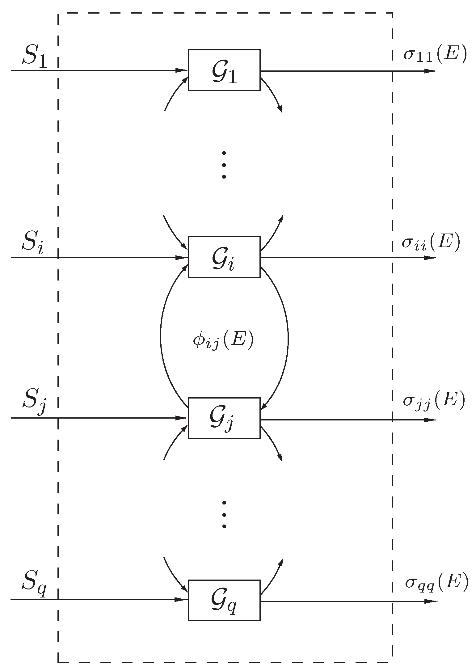
To formulate our state space thermodynamic model, consider the interconnected dynamical system
shown in
Figure 1 involving energy exchange between
q interconnected subsystems. Let
denote the energy (and hence a nonnegative quantity) of the
ith subsystem, let
denote the external power (heat flux) supplied to (or extracted from) the
ith subsystem, let
,
, denote the net instantaneous rate of energy (heat) flow from the
jth subsystem to the
ith subsystem, and let
, denote the instantaneous rate of energy (heat) dissipation from the
ith subsystem to the environment. Here, we assume that
,
,
, and
,
, are locally Lipschitz continuous on
and
, are bounded piecewise continuous functions of time.
Figure 1.
Interconnected dynamical system .
Figure 1.
Interconnected dynamical system .
An
energy balance for the
ith subsystem yields
or, equivalently, in vector form,
where
,
, is the system energy state,
,
, is the system dissipation,
,
, is the system heat flux, and
is such that
Since
,
, denotes the net instantaneous rate of energy flow from the
jth subsystem to the
ith subsystem, it is clear that
,
,
,
, which further implies that
,
.
Note that Equation (
2) yields a conservation of energy equation and implies that the energy stored in the
ith subsystem is equal to the external energy supplied to (or extracted from) the
ith subsystem plus the energy gained by the
ith subsystem from all other subsystems due to subsystem coupling minus the energy dissipated from the
ith subsystem to the environment. Equivalently, Equation (
2) can be rewritten as
or, in vector form,
where
, yielding a
power balance equation that characterizes energy flow between subsystems of the interconnected dynamical system
. We assume that
, whenever
,
,
, and
, whenever
,
. The above constraint implies that if the energy of the
ith subsystem of
is zero, then this subsystem cannot supply any energy to its surroundings or dissipate energy to the environment. In this case,
, is essentially nonnegative [
12]. Thus, if
, then, by Proposition 2.1, the solutions to Equation (
6) are nonnegative for all nonnegative initial conditions. See [
4,
11,
12] for further details.
Since our thermodynamic compartmental model involves intercompartmental flows representing energy transfer between compartments, we can use graph-theoretic notions with
undirected graph topologies (
i.e., bidirectional energy flows) to capture the compartmental system interconnections. Graph theory [
13,
14] can be useful in the analysis of the connectivity properties of compartmental systems. In particular, an undirected graph can be constructed to capture a compartmental model in which the compartments are represented by nodes and the flows are represented by edges or arcs. In this case, the environment must also be considered as an additional node.
For the interconnected dynamical system
with the power balance Equation (
6), we define a
connectivity matrix such that for
,
,
if
and
otherwise, and
,
. (The negative of the connectivity matrix, that is,
, is known as the graph Laplacian in the literature.) Recall that if rank
, then
is strongly connected [
4] and energy exchange is possible between any two subsystems of
.
The next definition introduces a notion of entropy for the interconnected dynamical system .
Definition 3.1 Consider the interconnected dynamical system with the power balance Equation (6). A continuously differentiable, strictly concave function is called the entropy function of ifand if and only if with , , .
It follows from Definition 3.1 that for an
isolated system , that is,
and
, the entropy function of
is a nondecreasing function of time. To see this, note that
where
and where we used the fact that
,
,
,
.
Proposition 3.1 Consider the isolated (i.e., and ) interconnected dynamical system with the power balance Equation (6). Assume that rank and there exists an entropy function of . Then, for all if and only if . Furthermore, the set of nonnegative equilibrium states of Equation (6) is given by .
Proof. If
, then
for all
, which implies that
for all
. Conversely, assume that
for all
, and, since
is an entropy function of
, it follows that
where we have used the fact that
for all
. Hence,
for all
. Now, the result follows from the fact that rank
. □
Theorem 3.1 Consider the isolated (i.e., and ) interconnected dynamical system with the power balance Equation (6). Assume that rank and there exists an entropy function of . Then the isolated system is globally semistable with respect to .
Proof. Since
is essentially nonnegative, it follows from Proposition 2.1 that
,
, for all
. Furthermore, note that since
,
, it follows that
,
. In this case,
,
, which implies that
,
, is bounded for all
. Now, it follows from Equation (
8) that
,
, is a nondecreasing function of time, and hence, by the Krasovskii–LaSalle theorem [
7],
as
. Next, it follows from Equation (
8), Definition 3.1, and the fact that rank
, that
.
Now, let
and consider the continuously differentiable function
defined by
where
. Next, note that
,
, and, since
is a strictly concave function,
, which implies that
admits a local minimum at
. Thus,
, there exists 0 such that
,
, and
for all
, which shows that
is a Lyapunov function for
and
is a Lyapunov stable equilibrium of
. Finally, since, for every
,
as
and every equilibrium point of
is Lyapunov stable, it follows from Proposition 2.2 that
is globally semistable with respect to
. □
In classical thermodynamics, the partial derivative of the system entropy with respect to the system energy defines the reciprocal of the system temperature. Thus, for the interconnected dynamical system
,
represents the temperature of the
ith subsystem. Equation (
7) is a manifestation of the
second law of thermodynamics and implies that if the temperature of the
jth subsystem is greater than the temperature of the
ith subsystem, then energy (heat) flows from the
jth subsystem to the
ith subsystem. Furthermore,
if and only if
with
,
,
, implies that temperature equality is a necessary and sufficient condition for thermal equilibrium. This is a statement of the
zeroth law of thermodynamics. As a result, Theorem 3.1 shows that, for a strongly connected system
, the subsystem energies converge to the set of equilibrium states where the temperatures of all subsystems are equal. This phenomenon is known as
equipartition of temperature [
4] and is an emergent behavior in thermodynamic systems. In particular, all the system energy is eventually transferred into heat at a uniform temperature, and hence, all dynamical processes in
(system motions) would cease.
The following result presents a sufficient condition for energy equipartition of the system, that is, the energies of all subsystems are equal. This state of energy equipartition is uniquely determined by the initial energy in the system.
Theorem 3.2 Consider the isolated (i.e., and ) interconnected dynamical system with the power balance Equation (6). Assume that rank and there exists a continuously differentiable, strictly concave function such that the entropy function of is given by . Then, the set of nonnegative equilibrium states of Equation (6) is given by and is semistable with respect to . Furthermore, as and is a semistable equilibrium state of .
Proof. First, note that since
is a continuously differentiable, strictly concave function, it follows that
which implies that Equation (
7) is equivalent to
and
if and only if
with
,
,
. Hence,
is an entropy function of
. Next, with
, it follows from Proposition 3.1 that
. Now, it follows from Theorem 3.1 that
is globally semistable with respect to
. Finally, since
and
as
, it follows that
as
. Hence, with
,
is a semistable equilibrium state of Equation (
6). □
If
, where
, so that
, then it follows from Theorem 3.2 that
and the isolated (
i.e.,
and
) interconnected dynamical system
with the power balance Equation (
6) is semistable. In this case, the absolute temperature of the
ith compartment is given by
. Similarly, if
, then it follows from Theorem 3.2 that
and the isolated (
i.e.,
and
) interconnected dynamical system
with the power balance Equation (
6) is semistable. In both cases,
as
. This shows that the steady-state energy of the isolated interconnected dynamical system
is given by
, and hence is uniformly distributed over all subsystems of
. This phenomenon is known as
energy equipartition [
4]. The aforementioned forms of
were extensively discussed in the recent book [
4] where
and
are referred to, respectively, as the entropy and the ectropy functions of the interconnected dynamical system
.
4. Work Energy, Gibbs Free Energy, Helmoholtz Free Energy, Enthalpy, and Entropy
In this section, we augment our thermodynamic energy flow model
with an additional (deformation) state representing subsystem volumes in order to introduce the notion of work into our thermodynamically consistent state space energy flow model. Specifically, we assume that each subsystem can perform (positive) work on the environment and the environment can perform (negative) work on the subsystems. The rate of work done by the
ith subsystem on the environment is denoted by
,
, the rate of work done by the environment on the
ith subsystem is denoted by
,
, and the volume of the
ith subsystem is denoted by
,
. The net work done by each subsystem on the environment satisfies
where
,
, denotes the
pressure in the
ith subsystem and
.
Furthermore, in the presence of work, the energy balance Equation (
5) for each subsystem can be rewritten as
where
,
,
, denotes the net instantaneous rate of energy (heat) flow from the
jth subsystem to the
ith subsystem,
,
, denotes the instantaneous rate of energy dissipation from the
ith subsystem to the environment, and, as in
Section 3,
,
, denotes the external power supplied to (or extracted from) the
ith subsystem. It follows from Equations (
10) and (
11) that positive work done by a subsystem on the environment leads to a decrease in the internal energy of the subsystem and an increase in the subsystem volume, which is consistent with the first law of thermodynamics.
The definition of entropy for
in the presence of work remains the same as in Definition 3.1 with
replaced by
and with all other conditions in the definition holding for every
. Next, consider the
ith subsystem of
and assume that
and
,
,
, are constant. In this case, note that
and
It follows from Equations (
10) and (
11) that, in the presence of work energy, the power balance Equation (
6) takes the new form involving energy and deformation states
where
,
,
,
,
, and
Note that
The power balance and deformation Equations (
14) and (15) represent a statement of the first law of thermodynamics. To see this, define the work
L done by the interconnected dynamical system
over the time interval
by
where
,
, is the solution to Equations (
14) and (15). Now, premultiplying Equation (
14) by
and using the fact that
, it follows that
where
denotes the variation in the total energy of the interconnected system
over the time interval
and
denotes the net energy received by
in forms other than work.
This is a statement of the
first law of thermodynamics for the interconnected dynamical system
and gives a precise formulation of the equivalence between work and heat. This establishes that heat and mechanical work are two different aspects of energy. Finally, note that Equation (15) is consistent with the classical thermodynamic equation for the rate of work done by the system
on the environment. To see this, note that Equation (15) can be equivalently written as
which, for a single subsystem with volume
V and pressure
p, has the classical form
It follows from Definition 3.1 and Equations (
14)–(
17) that the time derivative of the entropy function satisfies
Noting that
,
, is the infinitesimal amount of the net heat received or dissipated by the
ith subsystem of
over the infinitesimal time interval
, it follows from Equation (
23) that
Inequality (
24) is the classical
Clausius inequality for the variation of entropy during an infinitesimal irreversible transformation.
Note that for an
adiabatically isolated interconnected dynamical system (
i.e., no heat exchange with the environment), Equation (
23) yields the universal inequality
which implies that, for any dynamical change in an adiabatically isolated interconnected system
, the entropy of the final system state can never be less than the entropy of the initial system state. In addition, in the case where
,
, where
, it follows from Definition 3.1 and Equation (
23) that Inequality (
25) is satisfied as a strict inequality for all
. Hence, it follows from Theorem 2.15 of [
4] that the adiabatically isolated interconnected system
does not exhibit Poincaré recurrence in
.
Next, we define the
Gibbs free energy, the
Helmholtz free energy, and the
enthalpy functions for the interconnected dynamical system
. For this exposition, we assume that the entropy of
is a sum of individual entropies of subsystems of
, that is,
,
. In this case, the Gibbs free energy of
is defined by
the Helmholtz free energy of
is defined by
and the enthalpy of
is defined by
Note that the above definitions for the Gibbs free energy, Helmholtz free energy, and enthalpy are consistent with the classical thermodynamic definitions given by
,
, and
, respectively. Furthermore, note that if the interconnected system
is
isothermal and
isobaric, that is, the temperatures of subsystems of
are equal and remain constant with
and the pressure
in each subsystem of
remains constant, respectively, then any transformation in
is reversible.
The time derivative of
along the trajectories of Equations (
14) and (15) is given by
which is consistent with classical thermodynamics in the absence of chemical reactions.
For an isothermal interconnected dynamical system
, the time derivative of
along the trajectories of Equations (
14) and (15) is given by
where
L is the net amount of work done by the subsystems of
on the environment. Furthermore, note that if, in addition, the interconnected system
is
isochoric, that is, the volumes of each of the subsystems of
remain constant, then
. As we see in the next section, in the presence of chemical reactions the interconnected system
evolves such that the Helmholtz free energy is minimized.
Finally, for the isolated (
and
) interconnected dynamical system
, the time derivative of
along the trajectories of Equations (
14) and (15) is given by
5. Chemical Equilibria, Entropy Production, Chemical Potential, and Chemical Thermodynamics
In its most general form thermodynamics can also involve reacting mixtures and combustion. When a chemical reaction occurs, the bonds within molecules of the
reactant are broken, and atoms and electrons rearrange to form
products. The thermodynamic analysis of reactive systems can be addressed as an extension of the compartmental thermodynamic model described in
Section 3 and
Section 4. Specifically, in this case the compartments would qualitatively represent different quantities in the same space, and the intercompartmental flows would represent transformation rates in addition to transfer rates. In particular, the compartments would additionally represent quantities of different chemical substances contained within the compartment, and the compartmental flows would additionally characterize transformation rates of reactants into products. In this case, an additional mass balance is included for addressing conservation of energy as well as conservation of mass. This additional mass conservation equation would involve the law of mass-action enforcing proportionality between a particular reaction rate and the concentrations of the reactants, and the law of superposition of elementary reactions ensuring that the resultant rates for a particular species is the sum of the elementary reaction rates for the species.
In this section, we consider the interconnected dynamical system
where each subsystem represents a substance or species that can exchange energy with other substances as well as undergo chemical reactions with other substances forming products. Thus, the reactants and products of chemical reactions represent subsystems of
with the mechanisms of heat exchange between subsystems remaining the same as delineated in
Section 3. Here, for simplicity of exposition, we do not consider work done by the subsystem on the environment or work done by the environment on the system. This extension can be easily addressed using the formulation in
Section 4.
To develop a dynamical systems framework for thermodynamics with chemical reaction networks, let
q be the total number of species (
i.e., reactants and products), that is, the number of subsystems in
, and let
,
, denote the
jth species. Consider a single chemical reaction described by
where
,
,
, are the
stoichiometric coefficients and
k denotes the
reaction rate. Note that the values of
corresponding to the products and the values of
corresponding to the reactants are zero. For example, for the familiar reaction
,
, and
denote the species
,
, and
, respectively, and
,
,
,
,
, and
.
In general, for a reaction network consisting of
reactions, the
ith reaction is written as
where, for
,
is the reaction rate of the
ith reaction,
is the reactant of the
ith reaction, and
is the product of the
ith reaction. Each stoichiometric coefficient
and
is a nonnegative integer. Note that each reaction in the reaction network given by Equation (
35) is represented as being irreversible.
Irreversibility here refers to the fact that part of the chemical reaction involves generation of products from the original reactants. Reversible chemical reactions that involve generation of products from the reactants and vice versa can be modeled as two irreversible reactions, one involving generation of products from the reactants and the other involving generation of the original reactants from the products. Hence, reversible reactions can be modeled by including the reverse reaction as a separate reaction. The reaction network given by Equation (
35) can be written compactly in matrix-vector form as
where
is a column vector of species,
is a positive vector of reaction rates, and
and
are nonnegative matrices such that
and
,
,
.
Let
,
, denote the
mole number of the
jth species and define
. Invoking the
law of mass-action [
15], which states that, for an
elementary reaction, that is, a reaction in which all of the stoichiometric coefficients of the reactants are one, the rate of reaction is proportional to the product of the concentrations of the reactants, the species quantities change according to the dynamics [
11,
16]
where
and
For details regarding the law of mass-action and Equation (
37), see [
11,
15,
16,
17]. Furthermore, let
,
, denote the
molar mass (
i.e., the mass of one mole of a substance) of the
jth species, let
,
, denote the mass of the
jth species so that
,
,
, and let
. Then, using the transformation
, where
, Equation (
37) can be rewritten as the
mass balance
where
.
In the absence of nuclear reactions, the total mass of the species during each reaction in Equation (
36) is conserved. Specifically, consider the
ith reaction in Equation (
36) given by Equation (
35) where the mass of the reactants is
and the mass of the products is
. Hence, conservation of mass in the
ith reaction is characterized as
or, in general for Equation (
36), as
Note that it follows from Equations (
39) and (
41) that
.
Equation (
39) characterizes the change in masses of substances in the interconnected dynamical system
due to chemical reactions. In addition to the change of mass due to chemical reactions, each substance can exchange energy with other substances according to the energy flow mechanism described in
Section 3; that is, energy flows from substances at a higher temperature to substances at a lower temperature. Furthermore, in the presence of chemical reactions, the exchange of matter affects the change of energy of each substance through the quantity known as the
chemical potential.
The notion of the chemical potential was introduced by Gibbs in 1875–1878 [
8,
9] and goes far beyond the scope of chemistry, affecting virtually every process in nature [
18,
19,
20]. The chemical potential has a strong connection with the second law of thermodynamics in that
every process in nature evolves from a state of higher chemical potential towards a state of lower chemical potential. It was postulated by Gibbs [
8,
9] that the change in energy of a homogeneous substance is proportional to the change in mass of this substance with the coefficient of proportionality given by the chemical potential of the substance.
To elucidate this, assume the
jth substance corresponds to the
jth compartment and consider the rate of energy change of the
jth substance of
in the presence of matter exchange. In this case, it follows from Equation (
5) and Gibbs’ postulate that the rate of energy change of the
jth substance is given by
where
,
, is the chemical potential of the
jth substance. It follows from Equation (
42) that
is the chemical potential of a unit mass of the
jth substance. We assume that if
, then
,
, which implies that if the energy of the
jth substance is zero, then its chemical potential is also zero.
Next, using Equations (
39) and (
42), the energy and mass balances for the interconnected dynamical system
can be written as
where
and where
,
, and
are defined as in
Section 3. It follows from Proposition 1 of [
16] that the dynamics of Equation (44) are essentially nonnegative and, since
if
,
, it also follows that, for the isolated dynamical system
(
i.e.,
and
), the dynamics of Equations (
43) and (44) are essentially nonnegative.
Note that, for the
ith reaction in the reaction network given by Equation (
36), the chemical potentials of the reactants and the products are
and
, respectively. Thus,
is a restatement of the principle that a chemical reaction evolves from a state of a greater chemical potential to that of a lower chemical potential, which is consistent with the second law of thermodynamics. The difference between the chemical potential of the reactants and the chemical potential of the products is called
affinity [
21,
22] and is given by
Affinity is a driving force for chemical reactions and is equal to zero at the state of
chemical equilibrium. A nonzero affinity implies that the system in not in equilibrium and that chemical reactions will continue to occur until the system reaches an equilibrium characterized by zero affinity. The next assumption provides a general form for the inequalities (
45) and (
46).
Assumption 5.1 For the chemical reaction network (36) with the mass balance Equation (44), assume that for all andor, equivalently,where is the vector of chemical potentials of the substances of and is the affinity vector for the reaction network given by Equation (36).
Note that equality in Equation (
47) or, equivalently, in Equation (
48) characterizes the state of chemical equilibrium when the chemical potentials of the products and reactants are equal or, equivalently, when the affinity of each reaction is equal to zero. In this case, no reaction occurs and
,
.
Next, we characterize the entropy function for the interconnected dynamical system
with the energy and mass balances given by Equations (
43) and (44). The definition of entropy for
in the presence of chemical reactions remains the same as in Definition 3.1 with
replaced by
and with all other conditions in the definition holding for every
. Consider the
jth subsystem of
and assume that
and
,
,
, are constant. In this case, note that
and recall that
Next, it follows from Equation (
50) that the time derivative of the entropy function
along the trajectories of Equations (
43) and (44) is given by
For the isolated system
(
i.e.,
and
), the entropy function of
is a nondecreasing function of time and, using identical arguments as in the proof of Theorem 3.1, it can be shown that
as
for all
.
The entropy production in the interconnected system
due to chemical reactions is given by
If the interconnected dynamical system
is isothermal, that is, all subsystems of
are at the same temperature
where
is the system temperature, then it follows from Assumption 5.1 that
Note that since the affinity of a reaction is equal to zero at the state of a chemical equilibrium, it follows that equality in Equation (
54) holds if and only if
for some
and
.
Theorem 5.1 Consider the isolated (i.e., and ) interconnected dynamical system with the power and mass balances given by Equations (43) and (44). Assume that rank , Assumption 5.1 holds, and there exists an entropy function of . Then as , where , , is the solution to Equations (43) and (44) with the initial condition andwhere is the affinity vector of . Proof. Since the dynamics of the isolated system
are essentially nonnegative, it follows from Proposition 2.1 that
,
, for all
. Consider a scalar function
,
, and note that
and
,
,
. It follows from Equation (
41), Assumption 5.1, and
that the time derivative of
along the trajectories of Equations (
43) and (44) satisfies
which implies that the solution
,
, to Equations (
43) and (44) is bounded for all initial conditions
.
Next, consider the function
,
. Then it follows from Equations (
51) and (
56) that the time derivative of
along the trajectories of Equations (
43) and (44) satisfies
which implies that
is a nonincreasing function of time, and hence, by the Krasovskii–LaSalle theorem [
7],
as
. Now, it follows from Definition 3.1, Assumption 5.1, and the fact that rank
that
which proves the result. □
Theorem 5.1 implies that the state of the interconnected dynamical system converges to the state of thermal and chemical equilibrium when the temperatures of all substances of are equal and the masses of all substances reach a state where all reaction affinities are zero corresponding to a halting of all chemical reactions.
Next, we assume that the entropy of the interconnected dynamical system
is a sum of individual entropies of subsystems of
, that is,
,
. In this case, the Helmholtz free energy of
is given by
If the interconnected dynamical system
is isothermal, then the derivative of
along the trajectories of Equations (
43) and (44) is given by
with equality in Equation (
60) holding if and only if
for some
and
, which determines the state of chemical equilibrium. Hence, the Helmholtz free energy of
evolves to a minimum when the pressure and temperature of each subsystem of
are maintained constant, which is consistent with classical thermodynamics. A similar conclusion can be arrived at for the Gibbs free energy if work energy considerations to and by the system are addressed. Thus, the Gibbs and Helmholtz free energies are a measure of the tendency for a reaction to take place in the interconnected system
, and hence, provide a measure of the work done by the interconnected system
.
6. Conclusion and Opportunities for Future Research
In this paper, we developed a system-theoretic perspective for classical thermodynamics and chemical reaction processes. In particular, we developed a nonlinear compartmental model involving heat flow, work energy, and chemical reactions that captures all of the key aspects of thermodynamics, including its fundamental laws. In addition, we showed that the interconnected compartmental model gives rise to globally semistable equilibria involving states of temperature equipartition. Finally, using the notion of the chemical potential, we combined our heat flow compartmental model with a state space mass-action kinetics model to capture energy and mass exchange in interconnected large-scale systems in the presence of chemical reactions. In this case, it was shown that the system states converge to a state of temperature equipartition and zero affinity.
The underlying intention of this paper as well as [
4,
5,
6] has been to present one of the most useful and general physical branches of science in the language of dynamical systems theory. In particular, our goal has been to develop a dynamical system formalism of thermodynamics using a large-scale interconnected systems theory that bridges the gap between classical and statistical thermodynamics. The laws of thermodynamics are among the most firmly established laws of nature, and it is hoped that this work will help to stimulate increased interaction between physicists and dynamical systems and control theorists. Besides the fact that irreversible thermodynamics plays a critical role in the understanding of our physical universe, it forms the underpinning of several fundamental life science and engineering disciplines, including biological systems, physiological systems, neuroscience, chemical reaction systems, ecological systems, demographic systems, transportation systems, network systems, and power systems, to cite but a few examples.
An important area of science where the dynamical system framework of thermodynamics can prove invaluable is in neuroscience. Advances in neuroscience have been closely linked to mathematical modeling beginning with the integrate-and-fire model of Lapicque [
23] and proceeding through the modeling of the action potential by Hodgkin and Huxley [
24] to the current era of mathematical neuroscience; see [
25,
26] and the numerous references therein. Neuroscience has always had models to interpret experimental results from a high-level complex systems perspective; however, expressing these models with dynamic equations rather than words fosters precision, completeness, and self-consistency. Nonlinear dynamical system theory, and in particular system thermodynamics, is ideally suited for rigorously describing the behavior of large-scale networks of neurons.
Merging the two universalisms of thermodynamics and dynamical systems theory with neuroscience can provide the theoretical foundation for understanding the network properties of the brain by rigorously addressing large-scale interconnected biological neuronal network models that govern the neuroelectronic behavior of biological excitatory and inhibitory neuronal networks [
27]. As in thermodynamics, neuroscience is a theory of large-scale systems wherein graph theory can be used in capturing the connectivity properties of system interconnections, with neurons represented by nodes, synapses represented by edges or arcs, and synaptic efficacy captured by edge weighting giving rise to a weighted adjacency matrix governing the underlying directed graph network topology. However, unlike thermodynamics, wherein energy spontaneously flows from a state of higher temperature to a state of lower temperature, neuron membrane potential variations occur due to ion species exchanges which evolve from regions of higher concentrations to regions of lower concentrations. And this evolution does not occur spontaneously but rather requires the opening and closing of specific gates within specific ion channels.
A particularly interesting application of nonlinear dynamical systems theory to the neurosciences is to study phenomena of the central nervous system that exhibit nearly discontinuous transitions between macroscopic states. A very challenging and clinically important problem exhibiting this phenomenon is the induction of general anesthesia [
28,
29,
30,
31,
32]. In any specific patient, the transition from consciousness to unconsciousness as the concentration of anesthetic drugs increases is very sharp, resembling a thermodynamic phase transition. In current clinical practice of general anesthesia, potent drugs are administered which profoundly influence levels of consciousness and vital respiratory (ventilation and oxygenation) and cardiovascular (heart rate, blood pressure, and cardiac output) functions. These variation patterns of the physiologic parameters (
i.e., ventilation, oxygenation, heart rate, blood pressure, and cardiac output) and their alteration with levels of consciousness can provide scale-invariant fractal temporal structures to characterize the degree of consciousness in sedated patients.
In particular, the degree of consciousness reflects the adaptability of the central nervous system and is proportional to the maximum work output under a fully conscious state divided by the work output of a given anesthetized state. A reduction in maximum work output (and oxygen consumption) or elevation in the anesthetized work output (or oxygen consumption) will thus reduce the degree of consciousness. Hence, the fractal nature (
i.e., complexity) of conscious variability is a self-organizing emergent property of the large-scale interconnected biological neuronal network since it enables the central nervous system to maximize entropy production and optimally dissipate energy gradients. In physiologic terms, a fully conscious healthy patient would exhibit rich fractal patterns in space (e.g., fractal vasculature) and time (e.g., cardiopulmonary variability) that optimize the ability for oxygenation and ventilation. Within the context of aging and complexity in acute illnesses, variation of physiologic parameters and their relationship to system complexity, fractal variability, and system thermodynamics have been explored in [
33,
34,
35,
36,
37,
38].
Merging system thermodynamics with neuroscience can provide the theoretical foundation for understanding the mechanisms of action of general anesthesia using the network properties of the brain. Even though simplified mean field models have been extensively used in the mathematical neuroscience literature to describe large neural populations [
26], complex large-scale interconnected systems are essential in identifying the mechanisms of action for general anesthesia [
27]. Unconsciousness is associated with reduced physiologic parameter variability, which reflects the inability of the central nervous system to adopt, and thus, decomplexifying physiologic work cycles and decreasing energy consumption (ischemia, hypoxia) leading to a decrease in entropy production. The degree of consciousness is a function of the numerous coupling of the network properties in the brain that form a complex large-scale, interconnected system. Complexity here refers to the quality of a system wherein interacting subsystems self-organize to form hierarchical evolving structures exhibiting emergent system properties; hence, a complex dynamical system is a system that is greater than the sum of its subsystems or parts. This complex system—involving numerous nonlinear dynamical subsystem interactions making up the system—has inherent emergent properties that depend on the integrity of the entire dynamical system and not merely on a mean field simplified reduced-order model.
Developing a dynamical system framework for neuroscience [
27] and merging it with system thermodynamics [
4,
5,
6] by embedding thermodynamic state notions (
i.e., entropy, energy, free energy, chemical potential,
etc.) will allow us to directly address the otherwise mathematically complex and computationally prohibitive large-scale dynamical models that have been developed in the literature. In particular, a thermodynamically consistent neuroscience model would emulate the clinically observed self-organizing spatio-temporal fractal structures that optimally dissipate energy and optimize entropy production in thalamocortical circuits of fully conscious patients. This thermodynamically consistent neuroscience framework can provide the necessary tools involving semistability, synaptic drive equipartitioning (
i.e., synchronization across time scales), energy dispersal, and entropy production for connecting biophysical findings to psychophysical phenomena for general anesthesia.
In particular, we conjecture that as the model dynamics transition to an aesthetic state the system will involve a reduction in system complexity—defined as a reduction in the degree of irregularity across time scales—exhibiting semistability and synchronization of neural oscillators (
i.e., thermodynamic energy equipartitioning). In other words, unconsciousness will be characterized by system decomplexification. In addition, connections between thermodynamics, neuroscience, and the arrow of time [
4,
5,
6] can be explored by developing an understanding of how the arrow of time is built into the very fabric of our conscious brain. Connections between thermodynamics and neuroscience is not limited to the study of consciousness in general anesthesia and can be seen in biochemical systems, ecosystems, gene regulation and cell replication, as well as numerous medical conditions (e.g., seizures, schizophrenia, hallucinations,
etc.), which are obviously of great clinical importance but have been lacking rigorous theoretical frameworks. This is a subject of current research.
