New Climatic Indicators for Improving Urban Sprawl: A Case Study of Tehran City

Abstract

In the modern world, the fine balance and delicate relationship between human society and the environment in which we exist has been affected by the phenomena of urbanisation and urban development. Today, various environmental factors give rise to horizontal dispersion, spread and growth of cities. One of the most important results of this is climatic change which is directly affected by the urban sprawl of every metropolis. The aim of this study is to identify the relationship between the various horizontally distributed components of Tehran city and changes in essential microclimate clusters, by means of the humidex index. Results showed that, when the humidex was calculated for each of the obtained clusters, it was evident that it had increased with time, in parallel with Shannon’s entropy, as a consequence of the average temperature and relative humidity of each cluster. At the same time, results have shown that both temperature and relative humidity of the study area are related with urban sprawl, urbanisation and development, as defined by Shannon’s entropy and, in consequence, with humidex. In consequence, this new concept must be considered in future research works to predict and control urban sprawl and microclimate conditions in cities.

1. Introduction

Since the beginning of time, Earth has been in a constant state of experimenting with Nature’s harmony in different internal and external processes, but since human beings arrived on the scene, several new phenomena have produced effects that the planet has not been able to cope with [1]. To overcome this problem, there are various ways to achieve equilibrium, like population training in concepts such as energy conservation, recycling and reuse, tolerance and sharing. Despite all this, attaining optimum methods of reaching Earth’s perfect state of equilibrium, numerous research works were undertaken to look for suitable methodologies for sustainable town planning. Among others, Zapf’s Law was one of the possible solutions since it was observed in natural processes and in social institutions [1]. Besides this, more research works tried to find out the rank and size scaling relationship by means of the so-called entropy maximising methods. Despite this, and except in a few works [2], they often failed in their attempts. Finally, in the most recent works, as a method of measuring the system’s disorderliness, the entropy concept was employed in environmental systems [3,4,5,6,7]. Thus, the entropy of an urban ecosystem can be defined as a parameter indicative of the disorder [8]. In particular, Shannon’s entropy shows that the concentration of a spatial variable in a city quantifies its urban sprawl. For example, entropy can be divided into entropy flow and entropy production [8], and increases with sprawl [9]. Consequently, four types of entropy can be obtained with positive and negative values being the final values of the total entropy of the system. Once the total entropy is obtained, its difference between two periods of time will show the tendency of the urban sprawl [10]. From these theoretical concepts, different case studies were conducted in cities all over the world. For example, a research work developed in 2007 [10] in Canada implemented a land use classification for the City of Calgary, and simulated the future land use pattern based on the interactions between these land uses and the transportation network. Its results showed an adequate methodology in land use classification from Landsat images and the eCognition software, and concluded that entropy will grow in Calgary during the period 1985–2001 as a clear consequence of population growth. Other works analysed urban sprawl by means of Shannon’s entropy in the city of Baguio (northern Philippines) in 2010 [11], and showed the adequacy of remote sensing, Geographical Information Systems and photogrammetric techniques to show built-up concentration. In 2011, in the City of Vadodara (India), the integration of remote sensing and Geographical Information System was analysed to detect urban sprawl [12]. Once again, its results showed an entropy growth from 1.50 to 2.16 between years 1978 and 2001. A later study in Jorhat district of Assam (India) [13] showed an entropy growth between 2.32 in 1996 and 2.49 in 2010, which are near the highest entropy value of 2.63 which was identified with a clearly dispersed development. In 2012, the City of Beijing (China) [8] had analysed the developmental degree of the urban ecosystem from 2000 to 2007. Their results showed that the flow changes are the main factors that affect the system entropy changes, and showed quantitative indicators of the system state as adjustable indicators, controllable indicators and indicators that are not easily regulated. The first one can be adjusted by policies like economic growth indicators; the second one can be controlled by administrative and engineering technical means, like population density; and finally, the third indicators are those which cannot be adjusted by technical or economical procedures, like total annual electricity consumption. Its results showed that once the regulation program was improved, a negative entropy flow can be obtained. The more recent research works were developed in Iranian cities. For example, in the Iranian City of Shiraz in 2011 [9], its growth patterns between 1976 and 2005 were analysed using the Geographical Information System. Its results showed that the built-up area increased by 145%, while the population grew by only 55% due to the significantly unplanned development, and the proliferation of low population density construction. More recently, in another Iranian city (Urmia) in 2012 [14], urban growth was analysed using methods like Holdern and Shannon’s entropy. Its results showed that the value of entropy was 1.3738 in 1989, while the maximum value was 1.3862, showing the urban sprawl and physical developments. Finally, the entropy value was 1.3231 in 2007, indicating that over 20 years, physical growth has been both in the sprawl as well as in compact form. Therefore, it was concluded that changing a central city into a multicentric one based on centralisation and multiplication of activities in subcentres is the solution for coping with urban sprawl.

In Iran, which is a developing country, many big, medium, and even small cities, for various reasons, are encountering rapid spatial growth or urban sprawl. Tehran, the capital of Iran, is recognised as one of these expanding cities due to it being the main destination of migrants, because of its several modernistic urban attractions, in addition to a rapid population growth, and is experiencing rapid physical and spatial expansion. This phenomenon has many adverse effects on different aspects of the city, such as: the loss of environs, agricultural lands and orchards [15,16,17,18,19], increasing air pollution [20], increasing socioeconomic inequality [21], and so on.

At the same time, one of the most important environmental issues that is happening in Tehran, like in other metropolitan centres in the world, is climate change, and subsequent bioclimatic boundary changes in microclimatology on an urban scale. To prevent dangerous health consequences of these microclimatic conditions over the population, and at the same time to improve urban sprawl, new weather indexes must be employed.

However, the purpose of this research is to analyse and evaluate the microclimate in Tehran according to the urban sprawl of the city in different study periods, and to define new indexes to be employed in decisions for improving urban sprawl.

2. Materials and Methods

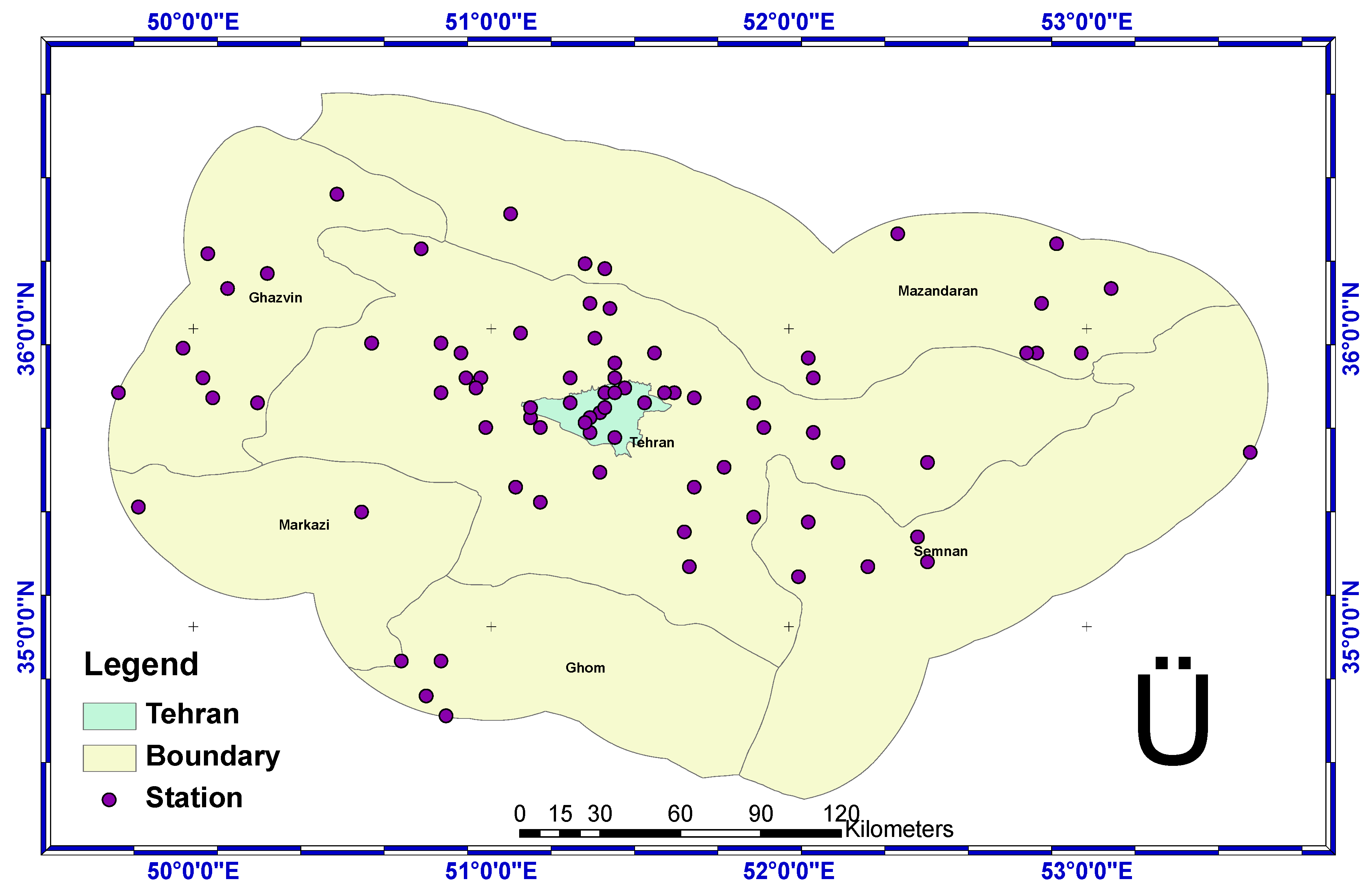
2.1. Studied Area

In this study, two types of data have been used. The first set of data includes temperature and relative humidity in 82 stations apart from Tehran, as is shown in Figure 1. The sampling period was from 1966 to 2005. The reason why temperature and relative humidity have been chosen is that these two variables play an important role in the bioclimatic conditions of urban and non-urban areas and, on the other hand, expansion of cities and urbanisation shows significant effects on the fluctuations of these variables.

The second set of studied data are the various components in relation to the urban sprawl of Tehran, such as the number of private cars per capita, city extent and population density. The information employed in this section was provided and received from some resources such as the Statistical Center of Iran, Tehran Municipality Planning and Studies Center, Fuel and Petroleum Products Company in Iran, Tehran Air Quality Control Company and the Department of Housing and Urban Development in Iran [22,23,24,25,26,27], as can be seen in Table 1.

Figure 1. Beyond the scope of Tehran, to reconstruct climate data.

Figure 1. Beyond the scope of Tehran, to reconstruct climate data.

Table 1. Changes in population, area, density and numbers of private cars in Tehran for different years [22,23,24,25,26,27].

Year	1921	1931	1941	1956	1966	1976	1986	1996	2000	2006
Population (million)	0.21	0.3	0.69	1.51	2.71	4.5	6.04	6.7	7.02	7.711
Area (hectarea)	720	2,420	4,500	10,000	19,000	32,000	62,000	73,950	78,900	80l000
Density (p/ha)	291.6	124	154	151	143	141	97.4	91	88.9	96.3
Private cars per 1,000 persons	-	-	-	5	25	31	61	74	83	90

Table 1. Changes in population, area, density and numbers of private cars in Tehran for different years [22,23,24,25,26,27].

Year	1921	1931	1941	1956	1966	1976	1986	1996	2000	2006
Population (million)	0.21	0.3	0.69	1.51	2.71	4.5	6.04	6.7	7.02	7.711
Area (hectarea)	720	2,420	4,500	10,000	19,000	32,000	62,000	73,950	78,900	80l000
Density (p/ha)	291.6	124	154	151	143	141	97.4	91	88.9	96.3
Private cars per 1,000 persons	-	-	-	5	25	31	61	74	83	90

2.2. Meteorological Data Reconstruction Methods

In the present work, 82 weather stations were employed, but only 38 had relative humidity sensors. At the same time, temperature and relative humidity data for all the stations were not sampled during the same study period (1966–2005). To solve this problem, a Kriging method was used to reconstruct the lack of data for each station. Daily data was reconstructed, and by using Kriging, 2,196 nodes of grid temperature and relative humidity components were reconstructed for each month. Finally, the output data was prepared for four studied periods, like 1975–1966, 1985–1976, 1995–1986 and 2005–1996.

2.3. Clustering Method and Preparation of Matrix Variables

In this section, the main stages of the clustering method will be enumerated as shown below:

A)

Preparing the raw data matrix;

B)

Calculating the raw data matrix;

C)

Forming the possible groups and calculating the Euclidian distance of each variable with its own group's average;

D)

Merging the groups by the method of minimum variance (the entering method) and determining the final grouping;

E)

Drawing the dendrogram which is the result of the merging of groups in several stages’

F)

Determining the location of clusters and junctions, and the final calculated grouping [28,29,30,31,32,33,34].

Cluster analysis consists of three types: two-step cluster analysis (T-SCA); K-means cluster analysis (K-MCA); and hierarchical cluster analysis (HCA). This last method will be employed in this research work with the help of the software MATLAB. After this, and based on the Euclidian distances between the amounts of climatic patterns and with the help of the integration method of Ward, the process of cluster analysis was completed to identify the effects of the urban sprawl of Tehran in different decades on the various microclimatic boundaries and cluster changes.

2.4. Shannon Entropy Indicator

The main objective of this study is to evaluate the irregularity or balance of a microclimatic nucleus in Tehran based on the urban sprawl of the city for different study periods. In particular, the reason why we consider a study area beyond Tehran City was to be able to compare microclimatic boundary changes for both natural and man-made areas.

Therefore, for this purpose, one of the strategies is to use the Shannon entropy method. For the performance of the Shannon entropy, it was necessary to specify clusters of Tehran microclimate for various periods. So, as mentioned in the previous section, microclimate clusters' preparation processes was described. Therefore, based on the Shannon entropy method, absolute entropy values were calculated by using Equation (1). In this equation, "Pi" value indicates each cluster's area for a specific period, and the aim of component "log (1/Pi)" is the total area of the region. It must be noted that the total area of the region is constant in different periods, but what constantly changes is the partial area of microclimatic clusters for each studied period.

The calculation assumes that an urban area is divided into n microclimatic zones, and that a variable, X, takes on a value X_i for any zone i $\in$ {1, 2,….,n}. Shannon’s entropy H_n is calculated as is shown in Equation (1):

$$H_n={\displaystyle \sum _i^n{P}_i\log (1/P_i)}$$

(1)

2.5. Estimate Thermal Comfort Proposal Indicator

To forecast the expected weather conditions in each different zone of Teheran City, humidex index was selected [35,36]. This index is the combination of dry bulb air temperature and moist air relative humidity showing the outdoor air perception of citizens as a consequence of a lack of skin sweat evaporation during the hot and humid weather conditions. This index can be defined by means of Equation (2):

(2)

where t is the moist air temperature (°C)

Finally, to understand the meaning of the humidex values obtained in this work, it is needed to revise its scale, as is shown in Table 2.

Table 2. Humidex scale.

Humidex range	Thermal comfort level
Less than 29 °C,	no discomfort
30 °C-39 °C,	some discomfort
40 °C-45 °C,	great discomfort
45 °C-54 °C,	dangerous
Above 54 °C,	heat stroke imminent

Table 2. Humidex scale.

Humidex range	Thermal comfort level
Less than 29 °C,	no discomfort
30 °C-39 °C,	some discomfort
40 °C-45 °C,	great discomfort
45 °C-54 °C,	dangerous
Above 54 °C,	heat stroke imminent

3. Results and Discussion

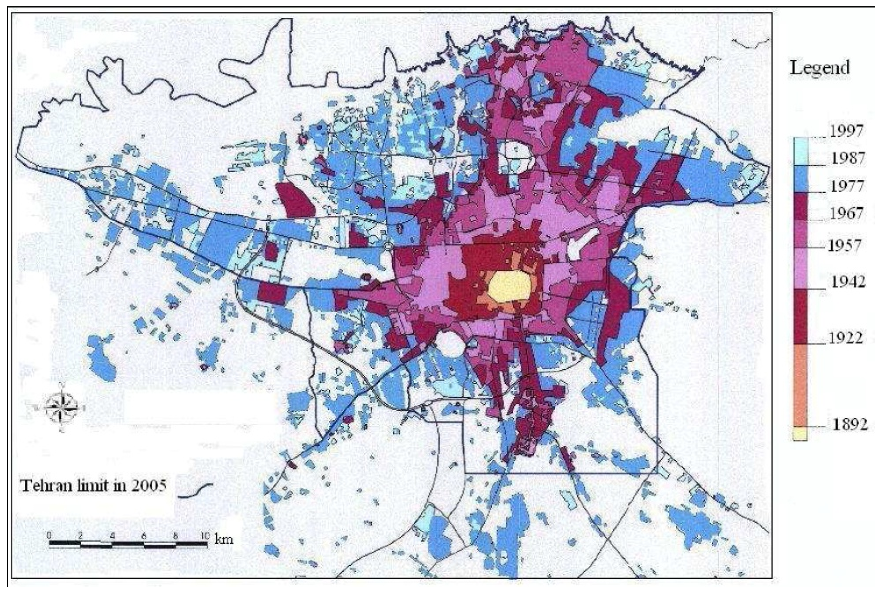
3.1. Urban Sprawl in Tehran

As is well known, urban sprawl is manifest when the growth of population is less than the growth in physical development. On the basis of this concept, the process of expansion of Tehran over different periods of time has shown that, in the last twenty years, this city experiences opposite processes of expansion and disintegration. To understand these concepts, it is necessary to look back and review the history of Tehran. In the initial stages, in Agha Mohammad Khan’s period (1822), the city of Tehran was recognised as Iran’s capital [28]. Furthermore, with six gateways, four quarters and 100,000 people surrounded by a wall, Tehran was placed in the first map of the city by French Mesu Kershish. At the same time, the city showed an area of 4 km², 1/3 of the area being filled with residential establishments and the remaining area dedicated to farming and gardening [29]. From that time, the city has experienced great changes time after time. For example, in 1921, the population was 210,000, and the city area was 7.2 km², which gave an extremely high population density of 291 persons per hectare.

As was explained before, the city’s growth has undergone an incredible acceleration both in physical and population aspects from the 1920s. In 1956, when the first official census was taken, it showed a population of 1,510,000 and a city area of 100 km² [23]. This growth continued with an incrementing intensity during the following decades.

As a consequence of this extremely prolific city growth, a council for the supervision on the expansion of Tehran, composed of different ministers and departmental managers, was nominated to act under the supervision of the acting prime minister. The aim of this council was to prevent and control the irregular expansion, and to chalk out a plan for the city’s future in accordance with the Act signed in 1973. Despite this, this council could not reach their objective and, in 1980, the Tehran municipality had to expand the scope of its services like, for example, to change the legal expansions from 225 to 520 km², and to increase the number of municipal districts from 12 to 20 [30]. From this time, a great number of villages (more than 120), along with two other cities, were absorbed (amalgamated) by Tehran, and this fast city growth has been repeated time after time till now. The latest official national census in 2006 showed that Tehran registered a population of 7,900,000, and a city area of 800 km². To sum up, we can say that in the last 85 years, Tehran’s population has multiplied by 37 and, what is more, its city area has multiplied by 100. Finally, it was recognised that the population density of the city during all these periods has showed a descending trend from 291 to 95 persons per hectare from 1921 to 2006, as can be seen in Table 1. Despite this, under this rapid physical growth, the city’s expansion was unplanned, dispersed and desultory, showing a clear example of sprawl, as can be seen in Figure 2.

Figure 2. The physical development of Tehran [18,26,27].

Figure 2. The physical development of Tehran [18,26,27].

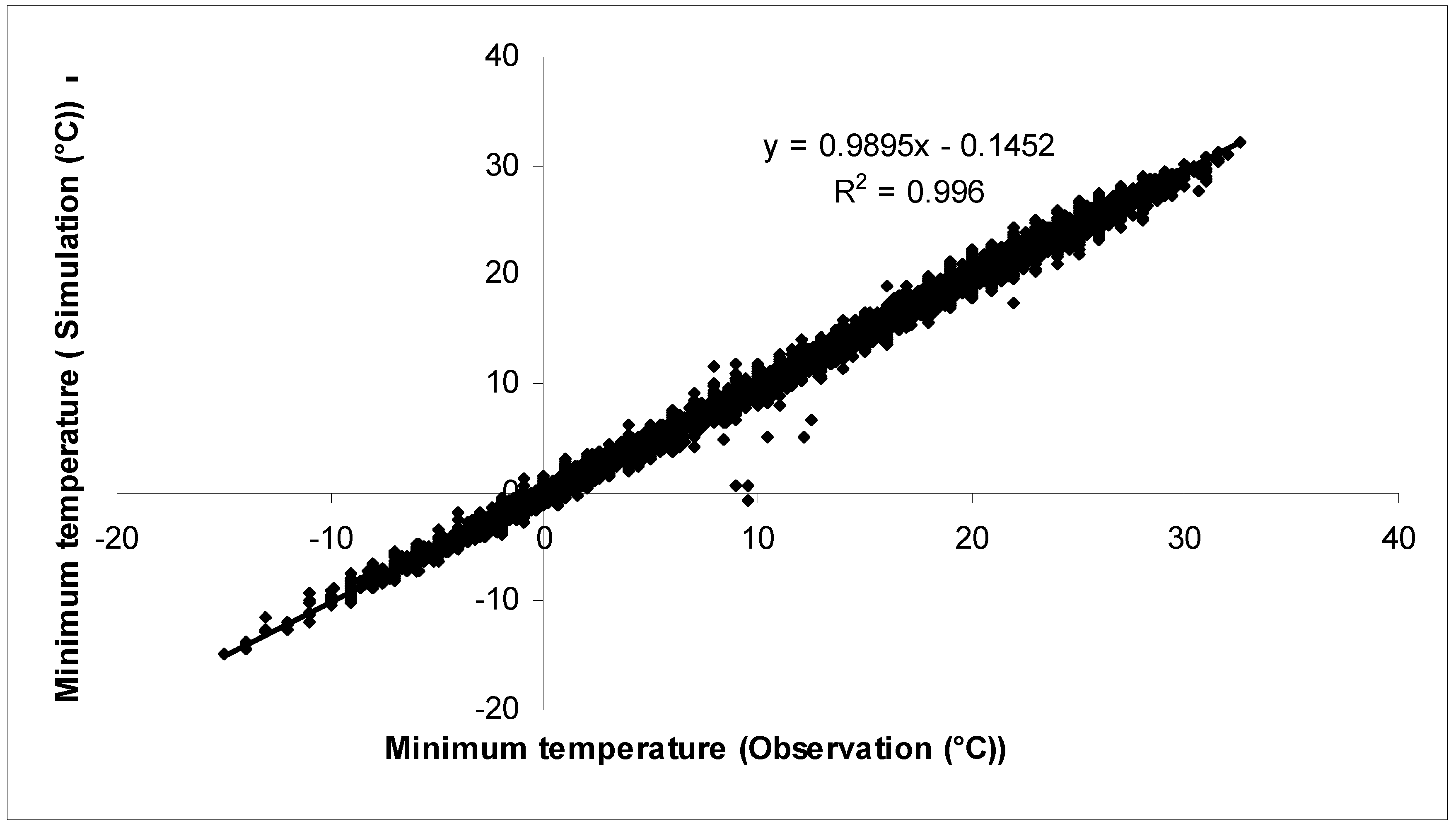
3.2. Validation of Simulated Data

As described earlier, after restoring data from each station by using Kriging, reconstructed data were validated to evaluate this method at a significance level. However, what was obtained from the results indicated that Kriging-observed data in respect of simulated data has the highest correlation and coincidence.

In this research, due to the large volume of data, and due to diagrams and the article's insufficient space, we cannot mention all stations. Nevertheless, as an example, Mehrabad station is shown in Figure 3, showing the highest significance level.

Figure 3. Comparison of daily minimum temperature reconstructed data using Kriging method, with experimental data at Mehrabad station.

Figure 3. Comparison of daily minimum temperature reconstructed data using Kriging method, with experimental data at Mehrabad station.

3.3. Essential Microclimates Indicators' Changes in Study Area

As was commented upon before, using monthly data for minimum and maximum temperatures and relative humidity, in a range from 51.05° East, to 51.65° East, and latitude 35.50° North to 35.85° North, was divided into different clusters. After this, eight microclimate clusters have been selected for four study periods, as can be seen in Figure 4.

On the basis of the first studied period (1966–1975), eight essential microclimate clusters were selected for the study area. Results showed that in this first studied period, the minimum temperature of 7.04 °C was obtained for the 8th cluster, and the maximum temperature was 22.91 °C for the 3rd one. The maximum relative humidity of 53.51% was obtained in the 6th cluster, and minimum relative humidity of 33.44% was estimated for cluster 1, as can be seen in Figure 4. In the second period (1976–1985), the minimum and maximum temperature values were found for the 8th and 4th clusters, with 15.80 °C and 22.55 °C, respectively. However, the minimum and maximum relative humidity of 36.84% and 55.03% were observed for clusters 1 and 4.

For the decade 1986–1995, the minimum temperature of 8.93 °C, and the maximum temperature of 22.75 °C, were calculated for the 8th and 1st clusters. Minimum and maximum relative humidity of 37.50% and 59.06% were observed in clusters 4 and 8, respectively. Finally, the 1996–2005 decade showed a minimum temperature of 10.49 °C and a maximum temperature of 22.75 °C, calculated for clusters 8 and 2. The maximum and minimum relative humidity with 54.59% and 35.18%, has been identified for clusters 8 and 1, as can be seen in Table 3.

Figure 4. Changes of essential microclimate clusters in the study area for different decades. (a) 1966-1975. (b) 1976-1985 (c) 1986-1995 (d) 1996-2005.

Figure 4. Changes of essential microclimate clusters in the study area for different decades. (a) 1966-1975. (b) 1976-1985 (c) 1986-1995 (d) 1996-2005.

It must be noted that in Figure 4, only the latest range for Tehran is given, which is related to the year 2008. This figure shows that the minimum temperature was obtained for cluster 8, and that the average temperature is increasing for all the periods and clusters, as can be seen in Table 3. Furthermore, it is clear that the temperature in the studied area has increased 0.72 °C per decade. Thus, in the last period, a temperature increment of 2.15 °C was obtained in respect of the first one. At the same time, the relative humidity showed the same increase process. In consequence, the overall mean of the average relative humidity has increased with an average of 0.40% per decade, and the difference between the last and the first decade was about 1.2%.

Table 3. Mean of minimum, maximum monthly values, and average temperature and relative humidity essential microclimates clusters.

Periods	Clusters	Min-Tem	Max-Hum	Max-Tem	Min-Hum	Ave-Tem	Ave-Hum
1965-1975	1	9.67	51.06	23.01	33.44	16.34	42.25
	2	9.15	51.1	22.16	34.82	15.655	42.96
	3	9.19	51.75	22.91	35.45	16.05	43.6
	4	9.04	52.52	21.82	36.84	15.43	44.68
	5	8.39	52.72	21.18	34.84	14.785	43.78
	6	8.08	53.51	20.07	38.29	14.075	45.9
	7	7.67	52.33	19.78	36.32	13.725	44.325
	8	7.04	53.09	18.76	37.72	12.9	45.405
1976-1985	1	10.11	54.53	22.33	36.84	16.22	45.685
	2	11.41	52.42	22.7	37.19	17.055	44.805
	3	10.95	53.83	23.11	39.86	17.03	46.845
	4	9.87	55.03	22.55	41.54	16.21	48.285
	5	11.05	52.9	22.34	41.5	16.695	47.2
	6	8.71	54.7	20.8	43.65	14.755	49.175
	7	8.53	53.48	19.92	42.17	14.225	47.825
	8	8.15	54.98	19.99	39.41	14.07	47.195
1986-1995	1	10.96	56.89	22.75	37.79	16.855	47.34
	2	10.44	55.89	21.96	42.1	16.2	48.995
	3	9.33	58.66	21.27	45.38	15.3	52.02
	4	11.07	53.65	21.62	37.5	16.345	45.575
	5	11.09	50.56	21.06	38.79	16.075	44.675
	6	10	52.27	19.97	41.25	14.985	46.76
	7	8.68	53.89	18.54	43.87	13.61	48.88
	8	9.63	59.06	20.94	38.8	15.285	48.93
1996-2005	1	12.12	53.77	23.15	35.18	17.635	44.475
	2	13.02	52.79	23.75	35.65	18.385	44.22
	3	12.45	51.97	23.31	36.74	17.88	44.355
	4	11.18	53.06	22.16	39.29	16.67	46.175
	5	12.69	49.47	21.77	36.71	17.23	43.09
	6	11.83	53.78	21.8	37.4	16.815	45.59
	7	11.63	51.89	20.73	39.78	16.18	45.835
	8	10.49	54.59	20.31	42.67	15.4	48.63

Table 3. Mean of minimum, maximum monthly values, and average temperature and relative humidity essential microclimates clusters.

Periods	Clusters	Min-Tem	Max-Hum	Max-Tem	Min-Hum	Ave-Tem	Ave-Hum
1965-1975	1	9.67	51.06	23.01	33.44	16.34	42.25
	2	9.15	51.1	22.16	34.82	15.655	42.96
	3	9.19	51.75	22.91	35.45	16.05	43.6
	4	9.04	52.52	21.82	36.84	15.43	44.68
	5	8.39	52.72	21.18	34.84	14.785	43.78
	6	8.08	53.51	20.07	38.29	14.075	45.9
	7	7.67	52.33	19.78	36.32	13.725	44.325
	8	7.04	53.09	18.76	37.72	12.9	45.405
1976-1985	1	10.11	54.53	22.33	36.84	16.22	45.685
	2	11.41	52.42	22.7	37.19	17.055	44.805
	3	10.95	53.83	23.11	39.86	17.03	46.845
	4	9.87	55.03	22.55	41.54	16.21	48.285
	5	11.05	52.9	22.34	41.5	16.695	47.2
	6	8.71	54.7	20.8	43.65	14.755	49.175
	7	8.53	53.48	19.92	42.17	14.225	47.825
	8	8.15	54.98	19.99	39.41	14.07	47.195
1986-1995	1	10.96	56.89	22.75	37.79	16.855	47.34
	2	10.44	55.89	21.96	42.1	16.2	48.995
	3	9.33	58.66	21.27	45.38	15.3	52.02
	4	11.07	53.65	21.62	37.5	16.345	45.575
	5	11.09	50.56	21.06	38.79	16.075	44.675
	6	10	52.27	19.97	41.25	14.985	46.76
	7	8.68	53.89	18.54	43.87	13.61	48.88
	8	9.63	59.06	20.94	38.8	15.285	48.93
1996-2005	1	12.12	53.77	23.15	35.18	17.635	44.475
	2	13.02	52.79	23.75	35.65	18.385	44.22
	3	12.45	51.97	23.31	36.74	17.88	44.355
	4	11.18	53.06	22.16	39.29	16.67	46.175
	5	12.69	49.47	21.77	36.71	17.23	43.09
	6	11.83	53.78	21.8	37.4	16.815	45.59
	7	11.63	51.89	20.73	39.78	16.18	45.835
	8	10.49	54.59	20.31	42.67	15.4	48.63

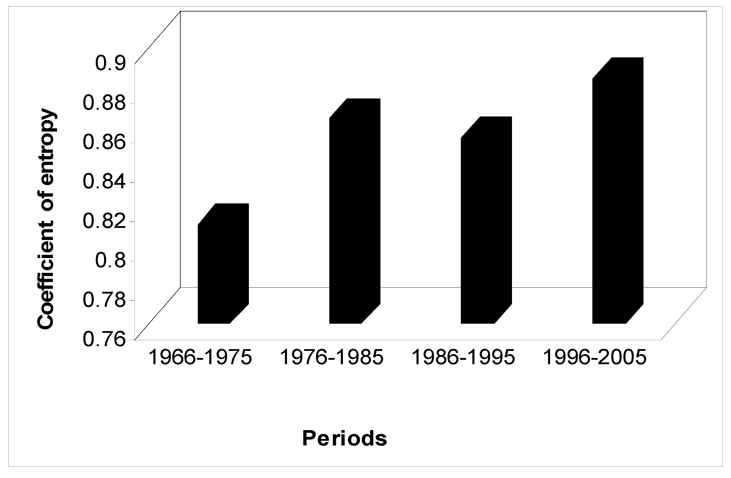
3.4. Calculating Nucleus Microclimate Entropy Values in Different Decades

In this section, Shannon entropy values were calculated for different microclimate clusters in each different decade. If we analyse the area variation of each different cluster, it can be concluded that cluster 1 showed the higher area in all the periods, and that it was followed by clusters 6 and 4, as we can see in Table 4. At the same time, the lowest area was related to clusters 7 and 8.

When absolute entropy was calculated in each cluster for the period 1965–1975, an average value of 0.81 was obtained. Furthermore, this value had increased to 0.86 in the second period, and had reduced to 0.85 in the third one. Finally, in the last studied period, Shannon entropy had reached its maximum value of 1, as can be seen in Figure 5.

Table 4. The area of essential microclimates of each cluster for different decades.

	Periods	Area in
Clusters		1966-1975	1976-1985	1986-1995	1996-2005
1		705.8	508.4	553.1	387.8
2		214.1	285.3	152.7	348.1
3		267.6	188.4	242.6	309.8
4		332.3	198.2	404.0	220.0
5		260.3	134.2	335.0	303.8
6		286.0	420.5	184.3	305.5
7		78.6	193.4	192.2	167.4
8		59.5	275.7	140.2	161.7
total		2,204.1	2,204.1	2,204.1	2,204.1

Table 4. The area of essential microclimates of each cluster for different decades.

	Periods	Area in
Clusters		1966-1975	1976-1985	1986-1995	1996-2005
1		705.8	508.4	553.1	387.8
2		214.1	285.3	152.7	348.1
3		267.6	188.4	242.6	309.8
4		332.3	198.2	404.0	220.0
5		260.3	134.2	335.0	303.8
6		286.0	420.5	184.3	305.5
7		78.6	193.4	192.2	167.4
8		59.5	275.7	140.2	161.7
total		2,204.1	2,204.1	2,204.1	2,204.1

As can be seen in Table 1, the population has increased since 1921. These increasing changes for the period 1966–1976 were 1.75 million people, and was 1.54 for the period 1976–1986. From 1986 to 1996, the lowest increment was reached with an increase of 0.66 million people. Finally, the highest increasing amount of people was obtained for the period 1996–2006 with 1.01 million people.

At the same time, an expansion for the Tehran area was obtained for each different period. In this sense, results have shown an increase of 13,000 hectares for the period 1966–1976, and 32,000 for study period 1976–1986. In the third period (1986–1998), this was the lowest sprawl period with about 11,950 hectares.

As a direct consequence of this effect, according to 1996 statistics, a clear lower population density in the end of this third period, rather than in 1986, was obtained. In particular, in the year 1996, a ratio of 6.5 people per hectare, which increased to 5.3 people per hectare in 2006 was obtained.

Another statistical index that can show us the tendency of urban sprawl in each period could be the density of number of vehicles per 1,000 people. When we applied this index to the third period, a clear deceleration could be observed. Results have shown values of 3, 30, 13 and 16 in each of the corresponding periods per 1,000 inhabitants.

Finally, all these indexes can justify and validate the use of Shannon entropy. In particular, a clear entropy reduction in the third period was obtained, as can be seen in Figure 5. Thus, it is expected that this urban sprawl deceleration is affected by the nucleus of essential microclimates of the study area, so it will be analysed in the next section.

Figure 5. Shannon entropy coefficient variation process for studied decades.

Figure 5. Shannon entropy coefficient variation process for studied decades.

3.5. Microclimate Changes and Urban Sprawl

In this section, we are going to analyse each different microclimate of each cluster to define the required energy for each one, and how it can influence urban sprawl.

In the initial state, it is interesting to confirm that relative humidity remains nearly constant in all clusters for each period, as can be seen in Figure 2. This relative humidity was about 42–46% in the first period, will increase between 45% and 49% in the second and third periods, and will decrease between 44% and 46% in the last period.

At the same time, from Figure 4, it can be observed that clusters 1 and 3 showed higher temperatures between 22 and 23 °C during the four periods. The resting clusters begin in a range between 19 °C and 20 °C and will increase to 21 °C in the resting periods.

As a consequence of the evolution of these two variables, the maximum humidex value will be between 20 and 25, which indicates a comfortable ambience. Despite this, it can be concluded that the humidex will remain constant in those clusters where the temperatures do not change with time (clusters 1 and 3) due to, as was explained before, relative humidity which does not change in each period, and that its effect on the humidex is clearly reduced when it is compared with dry bulb temperature. In the other clusters, due to its temperature increment with time, the humidex increased and, consequently, the global humidex in Tehran has been increased.

From these results, it can be concluded that this microclimate heating effect must be related with different urbanisation processes, and must be controlled to prevent the country entropy increase and its related future sprawl.

On the other hand, it can be concluded that the humidex is an interesting urban sprawl tool that can be employed to define the cluster evolution of other variables, like temperature, relative humidity and, indirectly, energy consumption, as the main causes for urban sprawl.

Figure 6. Humidex variation for different study periods.

Figure 6. Humidex variation for different study periods.

4. Conclusions

The present research work shows the irregularity of microclimates in different clusters, and its relationship with the Tehran urban sprawl. To achieve this objective, a cluster analysis method was used to clustering climatic data, while at the same time using the Shannon entropy method.

In an initial state, eight essential microclimate clusters in the City of Tehran were chosen for four study periods. In all these clusters, the results showed an average monthly temperature increase during the four study periods of 0.72 °C per decade. At the same time, relative humidity has also shown average increases of 0.40% per decade. When the humidex index was calculated for each of the obtained clusters, it was concluded that, due to relative humidity being nearly constant in each simulation period, and its effect on the humidex being clearly reduced when compared with the dry bulb temperature effect, it was concluded that the humidex had increased in each of the eight clusters with time. Despite the fact that its maximum obtained values were within the comfortable range till the present day, it can be an interesting way to define local microclimate dangers in cities.

From these results, it was obtained that both temperature and relative humidity of study area are related with urban sprawl and urban development. It seems evident that due to population increase, the use of fuels, greenhouse gases, and so on, would affect the increasing changes in humidity and temperature in the city. Consequently, humidex resulted to be a good indicator of the real effect of both variables, simultaneously.

When the average Shannon’s entropy was defined for each study period, a clear increment with time was obtained. Despite this, a temporal decrement during the third period was observed, and could be related with a lowest growth rate and personal car usage, when compared with the other time periods. Furthermore, these last indicators are quite likely to be a consequence of the war between Iran and Iraq that had a direct effect on Urban sprawl.

References and Notes

1. Fistola, R. The unsustainable city. Urban entropy and social capital: the needing of a new urban planning. Procedia. Eng. 2011, 21, 976–984. [Google Scholar] [CrossRef]
2. Chen, Y. The rank-size scaling law and entropy-maximizing principle. Physica A 2012, 391, 767–778. [Google Scholar] [CrossRef]
3. Liang, C.L.; Zhang, Z.L. Fuzzy assessment of water resources carrying capacity based on maximum entropy theory: A case study on Feicheng City. Water Res. Protection. 2006, 6, 35–37. [Google Scholar]
4. Jin, J.L.; Hong, T.Q.; Wng, W.S. Entropy and FAHP based fuzzy comprehensive evaluation model of water resources sustaining utilization. J. Hydroelectr. Eng. 2007, 26, 22–28. [Google Scholar]
5. Yang, W.; Tong, X.H.; Liu, M.L. Analysis of pattern change of entropy based land use. J. Tongji Univ. (Nat. Sci.). 2004, 31, 69–72. [Google Scholar]
6. Chen, H.; Liu, Y. Establishment and application of thermodynamics entropy to road traffic system. J. Hunan Univ. (Nat. Sci.). 2004, 31, 69–72. [Google Scholar]
7. He, D. Evaluation system build and policy study on regional circular economy development. Master's thesis; Wuhan University of Technology: Wuhan, China, 2006. http://www.dissertationtopic.net/doc/1094725 (Accessed 2013).
8. Wang, X.; Su, J.; Shan, S.; Zhang, Y. Urban ecological regulation based on information entropy at the town scale. A case study on Tongzhou district, Beijing City. Procedia. Env. Sci. 2012, 13, 1155–1164. [Google Scholar]
9. Sarvestania, M.S.; Ibrahima, Ab.L.; Kanarogloub, P. Three decades of urban growth in the city of Shiraz, Iran: A remote sensing and geographic information system applications. Cities 2011, 28, 320–329. [Google Scholar] [CrossRef]
10. Sun, H.; Forsythe, W.; Waters, N. Modeling Urban land Use Change and Urban Sprawl: Calgary, Alberta, Canada. Netw. Spat. Econ. 2007, 7, 353–376. [Google Scholar] [CrossRef]
11. Verzosa, L.C.O.; Gonzalez, R.M. Remote sensing, geographic information systems and Shannon’s Entropy: measuring urban sprawl in a mountainous environment. In ISPRS TC VII Symposium-100 Years ISPRS, Vienna, Austria, July 5–7, 2010. IAPRS 38, Part 7A.
12. Joshi, J.P.; Bhatt, B. Quantifying urban sprawl: A case study of Vadodara Taluka. Geo. Res. 2011, 1, 34–37. [Google Scholar]
13. Jyotishman, D.; Om, P.T.; Mohamed, L.K. Urban growth trend analysis using Shanon Entropy approach- A case study in North-East India. Int. J. Geol. 2012, 2, 1062–1068. [Google Scholar]
14. Mobaraki, O.; Mohammadi, J.; Zarabi, A. Urban form and sustainable development: the case of Urmia City. J. Geogr. Geol. 2012, 4, 1–12. [Google Scholar] [CrossRef]
15. Zhang, T. Land market forces and government’s role in sprawl, the case of China. Cities 2000, 17, 123–135. [Google Scholar] [CrossRef]
16. Jeffrey, A.C.; Foley, J.A. Agricultural land-use change in Brazilian Amazonia between 1980 and 1995: Evidence from integrated satellite and census data. Remote Sens. Environ. 2003, 87, 551–562. [Google Scholar]
17. Tan, M.; Li, X.; Xie, H.; Lu, C. Urban land expansion and arable land loss in China-A case study of Beijing–Tianjin–Hebei region. Land Use Policy 2005, 22, 187–196. [Google Scholar] [CrossRef]
18. Shahraki, S.Z. The analysis of Tehran urban sprawl and its effect on agricultural lands. M.A. Thesis in Geography and Urban Planning, University of Tehran, Iran, 2007. [Google Scholar]
19. Brabec, E.; Smith, C. Agricultural land fragmentation: the spatial effects of three land protection strategies in the eastern United States. Landsc. Urban Plan. 2002, 58, 255–268. [Google Scholar] [CrossRef]
20. Pourahmad, A.; Baghvand, A.; Shahraki, S.Z.; Givehchi, S. The impact of urban sprawl up on air pollution. Int. J. Environ. 2007, 1, 252–257. [Google Scholar]
21. Brueckner, J.K.; Largey, A.G. Social interaction and urban sprawl. J. Urban Econ. 2007, 10, 1–17. [Google Scholar] [CrossRef]
22. Pars Fuel. The Company of Fuel and Oil Products in Iran. data service. 2010; Tehran, Iran. (in Persian) [Google Scholar]
23. Iranian Statistics Center. Second Report in Censes of People and Housing. Tehran, Iran, 1986. (in Persian) [Google Scholar]
24. The Center of Studies and Planning of Tehran Municipality. Office of Air pollution and physical structure of Tehran city. Local data service. Tehran, Iran, 2005. [Google Scholar]
25. The Ministry of Housing and Urban Planning of Iran, report about the view of deconstruction from Tehran. Tehran, Iran, 2003.
26. Roshan, Gh.R.; Shahraki, S.Z.; Sauri, D.; Borna, R. Urban sprawl and climatic changes in tehran Iran. J. Environ. Health. Sci. Eng. 2010, 7, 43–52. [Google Scholar]
27. Roshan, Gh.R.; Rousta, I.; Ramesh, M. Studying the effects of urban sprawl of metropolis on tourism-climate index oscillation: A case study of Tehran city. J. Geo Reg. Plan. 2009, 2, 310–321. [Google Scholar]
28. Habibi, M.; Hurcade, B. Atlas of Tehran Metropolis, published by Analysis and Urban planning. Tehran municipality, 2005; 50–57. (in Persian) [Google Scholar]
29. Mehdizadeh, J. Period of rehabilitation and formation of Tehran metropolis (in Persian). J. Jostarhaye shahrsazi. 2003, 3, 26–32. [Google Scholar]
30. Dehaghani, N. An analysis of urban planning features in Iran, Science and Technology University of Iran Press. Tehran, Iran, 2004. (in Persian) [Google Scholar]
31. Sadeghi, R. Regional classification agriculture in southern Iran. J. Arid Environ. 2002, 50, 77–98. [Google Scholar] [CrossRef]
32. DeGaetano, A.T.; Shulman, M.D. A climatic classification of plant hardiness in the United States and Canada. Agr. Forest. Meteorol. 1990, 51, 333–351. [Google Scholar] [CrossRef]
33. Fovell, R.G.; Fovell, M.Y. Climate zones of the conterminous united states defined using cluster analysis. J. Climate 1993, 6, 2103–2135. [Google Scholar] [CrossRef]
34. Johnson, G.L.; Hanson, C.L.; Hardegree, S.P.; Ballard, E.B. Stochastic weather simulation: overview and analysis of two commonly used models. J. Appl. Meteorol. 1996, 35, 1878–1896. [Google Scholar] [CrossRef]
35. Carlucci, S.; Pagliano, L. A review of indices for the long-term evaluation of the general thermal comfort conditions in buildings. Energ. Build. 2012, 53, 194–205. [Google Scholar] [CrossRef]
36. Rainham, D.G.C.; Smoyer-Tomic, K.E. The role of air pollution in the relationship between a heat stress index and human mortality in Toronto. Environ. Res. 2003, 93, 9–19. [Google Scholar] [CrossRef]