Quantitative Analysis of Dynamic Behaviours of Rural Areas at Provincial Level Using Public Data of Gross Domestic Product


Abstract
:1. Introduction
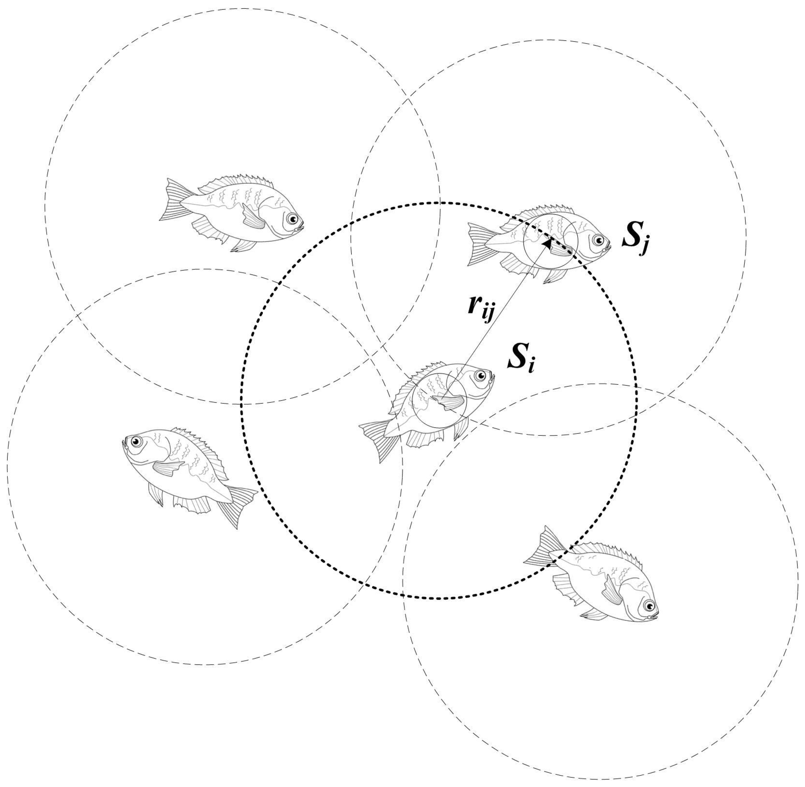
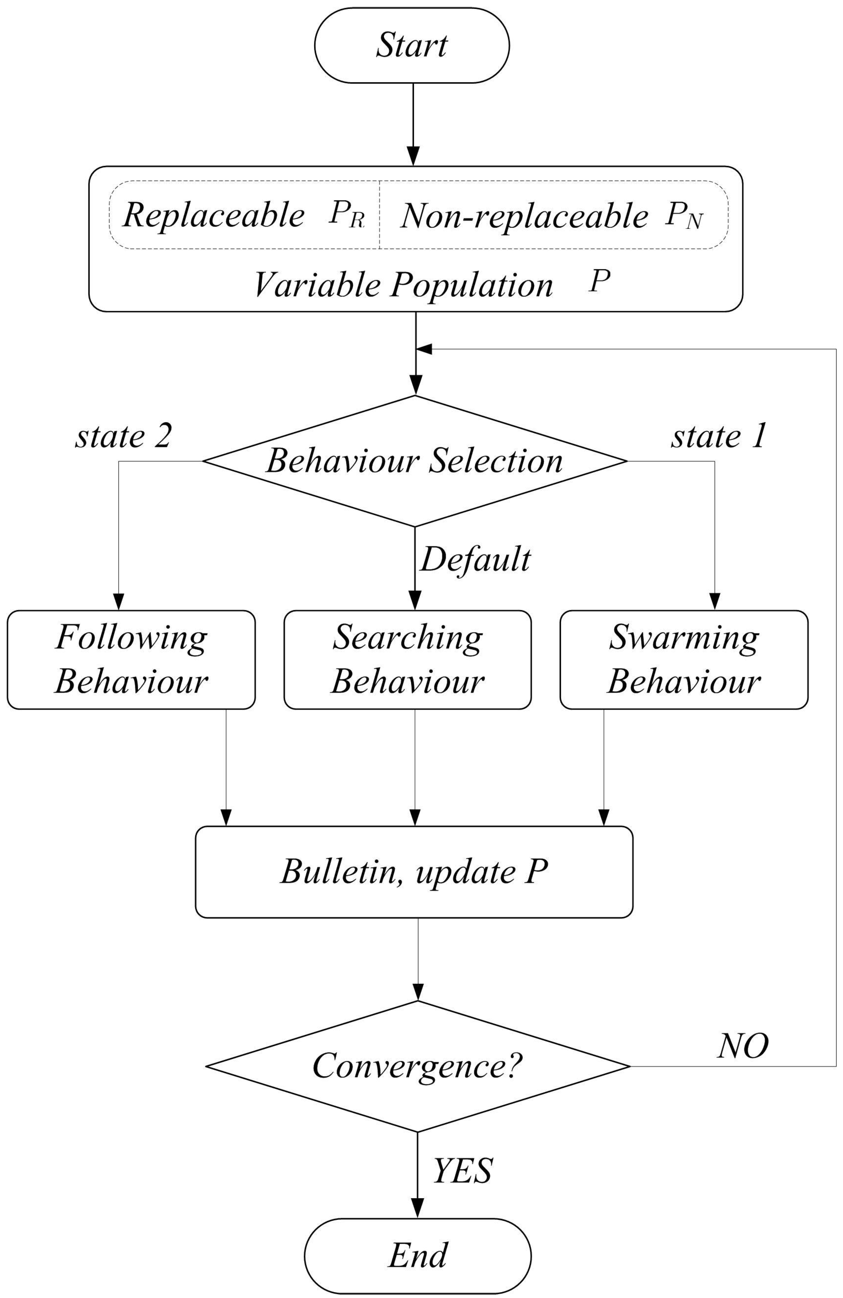
2. Variable Population Size Fish Swarm Algorithm
3. Quantitative Analysis Framework


| Conversion Factor | Emission Factor | Fraction of Carbon Oxidised | ||
|---|---|---|---|---|
| i | Fuel | () | () | |
| 0 | TCE | 29.27 | 24.74 | 0.90 |
| (A) Liquid | ||||
| Primary Fuel: | ||||
| 1 | Crude Oil | 42.62 | 20.00 | 0.98 |
| Secondary Fuel: | ||||
| 2 | Gasoline | 44.80 | 18.90 | 0.98 |
| 3 | Kerosene | 44.67 | 19.55 | 0.98 |
| 4 | Diesel Oil | 43.33 | 20.20 | 0.98 |
| 5 | Residual Fuel Oil | 40.19 | 21.10 | 0.98 |
| 6 | LPG | 47.31 | 17.20 | 0.98 |
| 7 | Naphtha | 45.01 | 20.00 | 0.80 |
| 8 | Bitumen | 40.19 | 22.00 | 1.00 |
| 9 | Lubricants | 40.19 | 20.00 | 0.50 |
| 10 | Other oil | 40.19 | 20.00 | 0.98 |
| (B) Solid | ||||
| Primary Fuel: | ||||
| 11 | Raw Coal | 20.52 | 24.74 | 0.90 |
| Secondary Fuel: | ||||
| 12 | Clean Coal | 20.52 | 24.74 | 0.90 |
| 13 | Washed Coal | 20.52 | 24.74 | 0.90 |
| 14 | House Coal | 20.52 | 24.74 | 0.90 |
| 15 | Coking Coal | 28.20 | 29.50 | 0.97 |
| 16 | Coal Tar | 28.00 | 22.00 | 0.75 |
| (C) Gaseous | ||||
| 17 | CNG | 48.00 | 15.30 | 0.99 |
- ∘
- E is the emission, ;
- ∘
- τ = 44/12 is the molecular weight ratio of to C (Conversion between C and can be calculated using the relative atomic weights of the carbon and oxygen atoms C = 12, O = 16. The atomic weight of carbon is 12 and that of is 12 + 16 + 16 = 44, i.e., one carbon and two oxygen atoms. To convert from C to thus requires multiplication by 44/12, or 3.67 [25].);
- ∘
- is the fraction of carbon oxidised (i = 1,2,..., ), = 17;
- ∘
- is the heat conversion factor, ;
- ∘
- is the carbon emission factor, which is considered as the carbon content per unit of energy for its close link between the carbon content and energy value of the fuel, ;
- ∘
- is the non-energy use, ;
- ∘
- is the apparent consumption, t;
- ∘
- is the energy production, t;
- ∘
- is the import energy, t;
- ∘
- is the export energy, t;
- ∘
- is the international bunkers, t;
- ∘
- is the stock change, t;
| j | Province | ||||||
|---|---|---|---|---|---|---|---|
| 1 | Beijing | 0.662 | 104880300 | 719.61 | 69430758.6 | 476.38182 | 165,916.0 |
| 2 | Tianjing | 0.947 | 63543800 | 910.42 | 60175978.6 | 862.16774 | 143,800.2 |
| 3 | Hebei | 1.727 | 161886100 | 1492.81 | 279577294.7 | 2578.08287 | 668,095.1 |
| 4 | Shanxi | 2.554 | 69387300 | 2288.87 | 177215164.2 | 5845.77398 | 423,484.4 |
| 5 | Neimenggu | 2.159 | 77618000 | 1887.32 | 167577262 | 4074.72388 | 400,453.0 |
| 6 | Liaoning | 1.617 | 134615700 | 1223.81 | 217673586.9 | 1978.90077 | 520,166.2 |
| 7 | Jiling | 1.444 | 64240600 | 885.93 | 92763426.4 | 1279.28292 | 221,673.2 |
| 8 | Heilongjiang | 1.290 | 83100000 | 865.90 | 107199000 | 1117.011 | 256,169.3 |
| 9 | Shanghai | 0.801 | 136981500 | 884.13 | 109722181.5 | 708.18813 | 262,198.9 |
| 10 | Jiangshu | 0.803 | 303126100 | 1149.44 | 243410258.3 | 923.00032 | 581,668.1 |
| 11 | Zhejiang | 0.782 | 214869200 | 1202.08 | 168027714.4 | 940.02656 | 401,529.4 |
| 12 | Anhui | 1.075 | 88741700 | 1106.81 | 95397327.5 | 1189.82075 | 227,967.3 |
| 13 | Fujian | 0.843 | 108231100 | 1098.56 | 91238817.3 | 926.08608 | 218,029.9 |
| 14 | Jiangxi | 0.928 | 64803300 | 942.16 | 60137462.4 | 874.32448 | 143,708.2 |
| 15 | Shandong | 1.100 | 310720600 | 1001.08 | 341792660 | 1101.188 | 816,768.7 |
| 16 | Henan | 1.219 | 184077800 | 1266.23 | 224390838.2 | 1543.53437 | 536,218.2 |
| 17 | Hubei | 1.314 | 113303800 | 1103.90 | 148881193.2 | 1450.5246 | 355,775.7 |
| 18 | Hunan | 1.225 | 111566400 | 975.49 | 136668840 | 1194.97525 | 326,592.3 |
| 19 | Guangdong | 0.715 | 356964600 | 1085.49 | 255229689 | 776.12535 | 609,912.5 |
| 20 | Guangxi | 1.106 | 71715800 | 1254.15 | 79317674.8 | 1387.0899 | 189,542.4 |
| 21 | Hainan | 0.875 | 14592300 | 979.24 | 12768262.5 | 856.835 | 30,511.8 |
| 22 | Chongqing | 1.267 | 50966600 | 1090.19 | 64574682.2 | 1381.27073 | 154,311.7 |
| 23 | Sichuan | 1.381 | 125062500 | 1156.37 | 172711312.5 | 1596.94697 | 412,721.6 |
| 24 | Guizhou | 2.875 | 33334000 | 2452.21 | 95835250 | 7050.10375 | 229,014.0 |
| 25 | Yunnan | 1.562 | 57001000 | 1654.94 | 89035562 | 2585.01628 | 212,764.9 |
| 26 | Xizang | 0 | 3959100 | 0 | 0 | 0 | 0 |
| 27 | Shaanxi | 1.281 | 68513200 | 1256.02 | 87765409.2 | 1608.96162 | 209,729.7 |
| 28 | Gansu | 2.013 | 31761100 | 2539.00 | 63935094.3 | 5111.007 | 152,783.4 |
| 29 | Qinhai | 2.935 | 9615300 | 4061.64 | 28220905.5 | 11920.9134 | 67,438.7 |
| 30 | Ningxia | 3.686 | 10985100 | 5084.09 | 40491078.6 | 18739.95574 | 96,760.5 |
| 31 | Xingjiang | 1.963 | 42034100 | 1331.24 | 82512938.3 | 2613.22412 | 197,178.1 |
| 9,232,883.4 |
- ∘
- is the total TCE emission estimation of the provincial rural areas, ;
- ∘
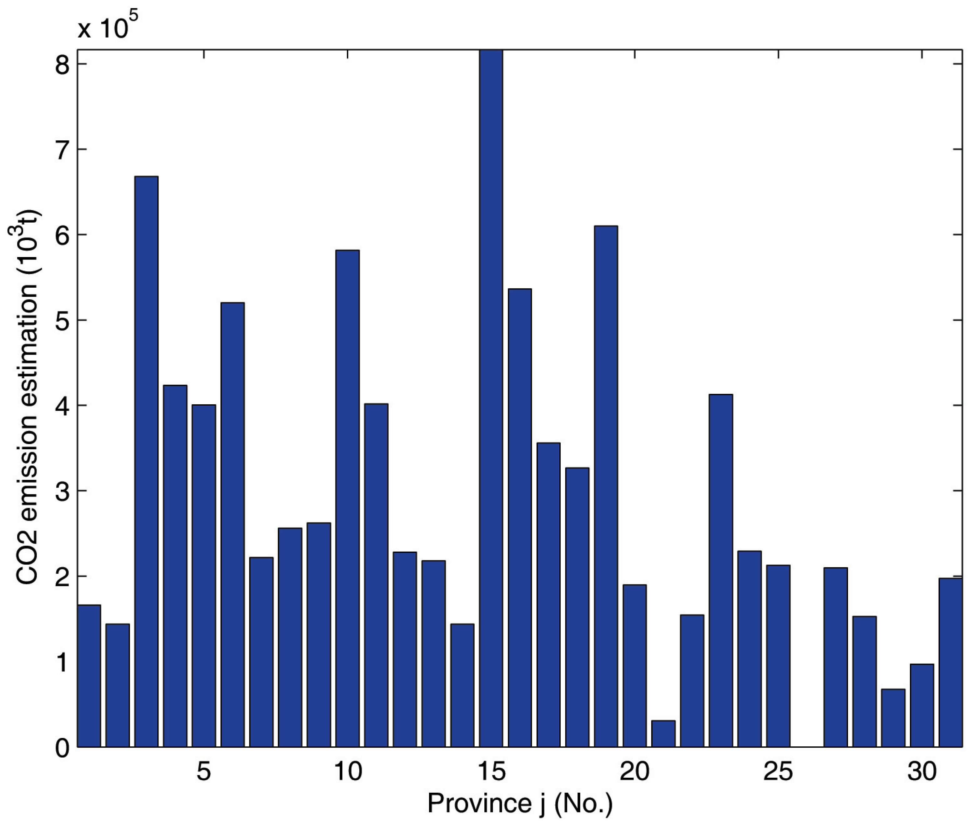
- is the emission estimation of province j by GDP, as listed in Table 2, ;
- ∘
- is the gross domestic product (GDP) of province j, ;
- ∘
- is the TCE energy consumption per GDP unit of province j, TCE/;
- ∘
- is the electricity consumption per GDP unit of province j, /;
- ∘
- is the ratio of electricity to TCE, which is 0.01182 in this case (Electricity is converted to TCE by the equation 104 = 1.229 TCE, that is, = 1.229/104 = 0.01182 [31]);
- ∘
- τ, , and are the molecular weight ratio of to C, the TCE fraction of carbon oxidised, the TCE heat conversion factor and the TCE carbon emission factor, as given in Table 1, j = 1,...,.
4. Multi-State Dynamic Behaviours Modelling
- ∘
- Θ is the functional region affecting index;
- ∘
- is the number of enterprises in the province j, is the number of the provinces;
- ∘
- is the total profits of province j, ;
- ∘
- is the non-agricultural employment of province j, persons;
- ∘
- = / is the population effect coefficient of province j, is the local non-agricultural population, is the population of province j, persons;
- ∘
- is the emission of province j, as listed in Table 2;
- ∘
- is the multi-state factor of province j, ∈ [-1,1], as defined in Equation (16), which is the normalised , and are the and values of . According to the historical data and statistics, is utilised to describe the MSS weighted behaviour of the uncertainty analysis;
- ∘
- β is the factor of the functional distance , β ∈ [0.5,3];
- ∘
- ϵ is the floating point relative accuracy, which prevents the singularity in case of the is approaching to 0 and Θ is approaching to ∞, numerically;
- ∘
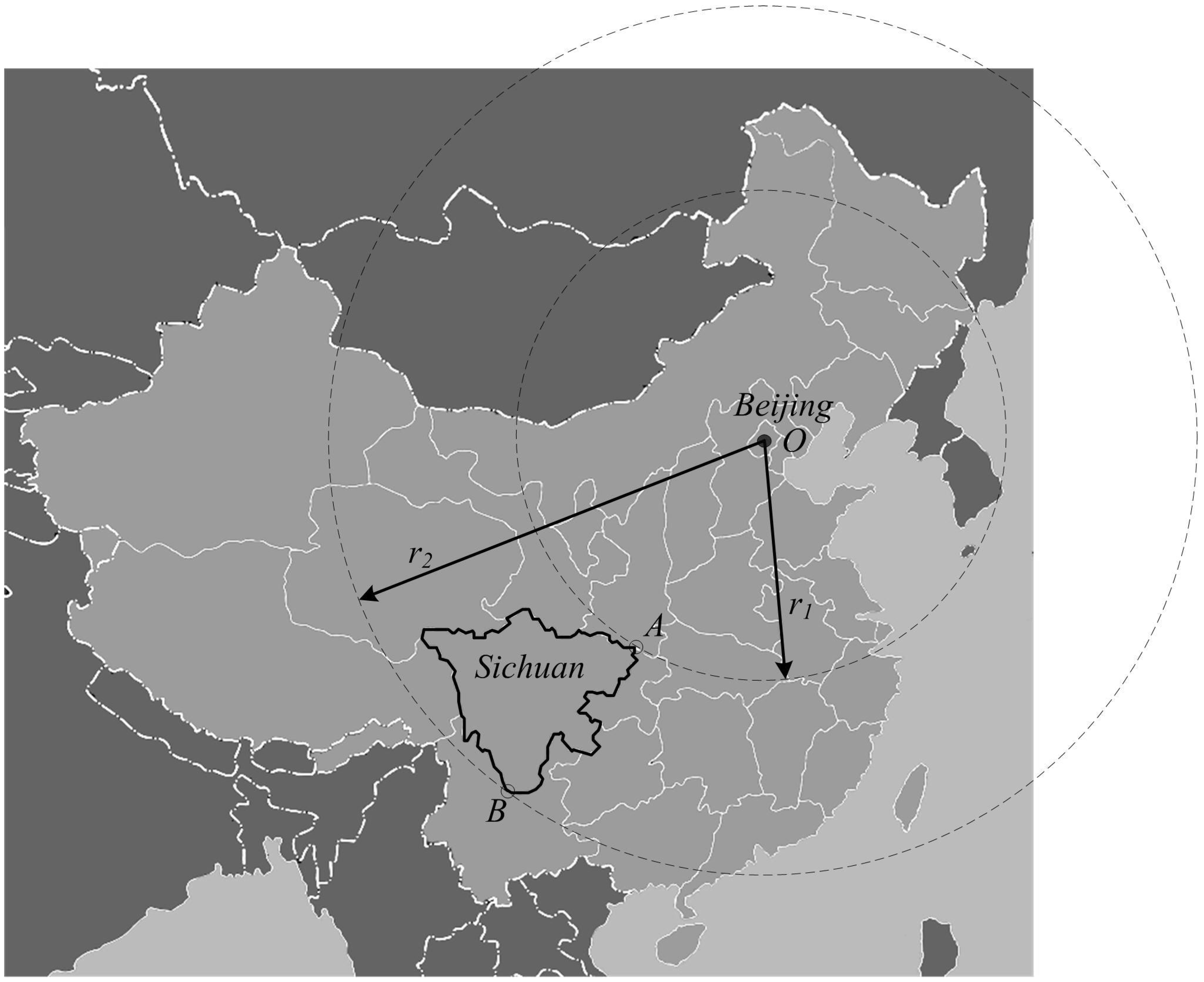
- is the mean value of point-to-point distance from the point O to each province j, as defined in Equation (17), kilometre (km).
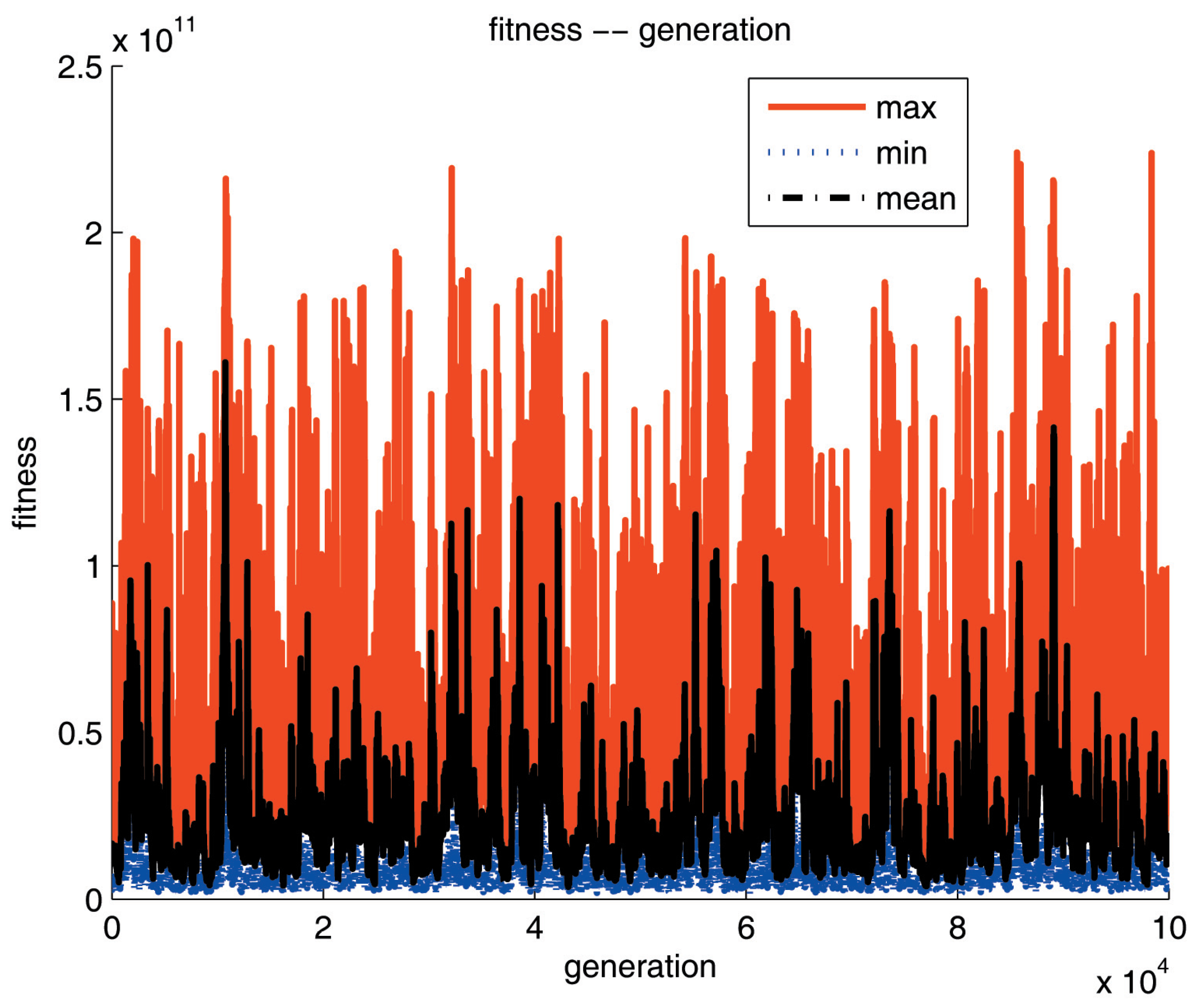
5. Fitness Function Definition
| No. j | Province | |||||||
|---|---|---|---|---|---|---|---|---|
| 1 | Beijing | 0.00 | 129.00 | 1695 | 1439 | 7205 | 5570000 | 123.38 |
| 2 | Tianjing | 49.45 | 168.99 | 1176 | 908 | 7950 | 7527900 | 133.12 |
| 3 | Hebei | 30.96 | 442.47 | 6989 | 2928 | 12447 | 13698400 | 316.85 |
| 4 | Shanxi | 162.97 | 781.31 | 3411 | 1539 | 4415 | 6342500 | 214.93 |
| 5 | Neimenggu | 206.83 | 1617.23 | 2414 | 1248 | 3993 | 7714400 | 104.57 |
| 6 | Liaoning | 228.33 | 789.91 | 4315 | 2591 | 21876 | 7815800 | 366.23 |
| 7 | Jiling | 689.29 | 1280.97 | 2734 | 1455 | 5257 | 3962300 | 126.99 |
| 8 | Heilongjiang | 884.94 | 1752.25 | 3825 | 2119 | 4392 | 15816900 | 155.99 |
| 9 | Shanghai | 976.53 | 1091.77 | 1888 | 1673 | 18792 | 9672400 | 304.01 |
| 10 | Jiangshu | 542.23 | 1059.09 | 7677 | 4169 | 65495 | 39729300 | 1104.06 |
| 11 | Zhejiang | 995.88 | 1434.05 | 5120 | 2949 | 58816 | 16342000 | 814.55 |
| 12 | Anhui | 571.47 | 1153.69 | 6135 | 2485 | 11392 | 6067300 | 210.8 |
| 13 | Fujian | 1276.24 | 1783.64 | 3604 | 1798 | 17212 | 8961100 | 380.06 |
| 14 | Jiangxi | 1069.41 | 1689.04 | 4400 | 1820 | 7367 | 5079600 | 178.56 |
| 15 | Shandong | 216.72 | 625.65 | 9417 | 4483 | 42629 | 39235600 | 912.7 |
| 16 | Henan | 420.97 | 932.24 | 9429 | 3397 | 18700 | 22877800 | 417.36 |
| 17 | Hubei | 851.83 | 1336.87 | 5711 | 2581 | 12067 | 9090300 | 235.9 |
| 18 | Hunan | 1127.46 | 1718.28 | 6380 | 2689 | 12391 | 6635600 | 225.55 |
| 19 | Guangdong | 1584.55 | 2230.41 | 9544 | 6048 | 52574 | 32726000 | 1493.38 |
| 20 | Guangxi | 1548.86 | 2166.34 | 4816 | 1838 | 5427 | 2311400 | 114.6 |
| 21 | Hainan | 2223.53 | 3046.98 | 854 | 410 | 548 | 807400 | 12.61 |
| 22 | Chongqing | 1071.13 | 1511.45 | 2839 | 1419 | 6119 | 3086800 | 132.13 |
| 23 | Sichuan | 1097.36 | 2011.97 | 8138 | 3044 | 13725 | 8445600 | 297.54 |
| 24 | Guizhou | 1382.45 | 1984.45 | 3793 | 1104 | 2676 | 1818300 | 73.53 |
| 25 | Yunnan | 1646.04 | 2522.81 | 4543 | 1499 | 3320 | 3101400 | 84.34 |
| 26 | Xizang | 1812.45 | 3418.07 | 287 | 65 | 88 | 45000 | 1.79 |
| 27 | Shaanxi | 443.33 | 1193.68 | 3762 | 1584 | 4025 | 10089900 | 131.83 |
| 28 | Gansu | 764.54 | 2032.18 | 2628 | 845 | 1940 | 1094600 | 69.13 |
| 29 | Qinhai | 1221.63 | 2406.28 | 554 | 227 | 515 | 1771700 | 17.42 |
| 30 | Ningxia | 774.43 | 1068.55 | 618 | 278 | 901 | 391300 | 25.89 |
| 31 | Xingjiang | 1677.43 | 3590.93 | 2131 | 845 | 1859 | 7795200 | 57.84 |
- ∘
- X = [, , ..., , ..., ] is the vector of the enterprise number, X ∼ . Let = [, , ..., , ..., ] and = [, , ..., , ..., ] be the mean and the standard deviation vectors of X, respectively, that is, ∼ , and are the mean and the standard deviation of ;
- ∘
- Y = [, , ..., , ..., ] is the vector of the total profits, Y ∼ . Let = [, , ..., , ..., ] and = [, , ..., , ..., ] be the mean and the standard deviation vectors of Y, respectively, such that ∼ , and are the mean and the standard deviation of ;
- ∘
- Z = [, , ..., , ..., ] is the vector of the non-agricultural employment, Z ∼ . Let = [, , ..., , ..., ] and = [, , ..., , ..., ] be the mean and the standard deviation vectors of Z, respectively, such that ∼ , and are the mean and the standard deviation of ;
- ∘
6. Empirical Results and Discussions
| max generations | 100,000 | |
| experiment number | 100 | |
| population | 60 | |
| non-replaceable population | 50 | |
| replaceable population | 10 | |
| CV () | 15% | |
| δ | iterate step | 0.5 |
| υ | visual | 2.5 |
| η | crowd | 0.618 |
| try number | 5 |

| No. j | Province | (%) | (%) | (%) | |||
|---|---|---|---|---|---|---|---|
| 1 | Beijing | 2103.37 | -70.81 | 5259913.76 | -5.57 | 121.52 | -1.50 |
| 2 | Tianjing | 7162.66 | -9.90 | 3875238.80 | -48.52 | 55.39 | -58.39 |
| 3 | Hebei | 5471.55 | -56.04 | 3607953.26 | -73.66 | 94.19 | -70.27 |
| 4 | Shanxi | 2828.75 | -35.93 | 1177466.56 | -81.44 | 64.13 | -70.16 |
| 5 | Neimenggu | 671.11 | -83.19 | 4232075.41 | -45.14 | 31.17 | -70.19 |
| 6 | Liaoning | 5099.33 | -76.69 | 5457102.47 | -30.18 | 102.12 | -72.12 |
| 7 | Jiling | 3598.66 | -31.55 | 1516642.78 | -61.72 | 19.86 | -84.36 |
| 8 | Heilongjiang | 2098.07 | -52.23 | 15558105.89 | -1.64 | 97.39 | -37.56 |
| 9 | Shanghai | 13194.87 | -29.78 | 2140995.88 | -77.86 | 177.82 | -41.51 |
| 10 | Jiangshu | 56854.80 | -13.19 | 23504968.27 | -40.84 | 603.88 | -45.30 |
| 11 | Zejiang | 20379.23 | -65.35 | 7582321.11 | -53.60 | 492.79 | -39.50 |
| 12 | Anhui | 9517.09 | -16.46 | 1358894.06 | -77.60 | 90.46 | -57.09 |
| 13 | Fujian | 16657.98 | -3.22 | 7250945.22 | -19.08 | 210.31 | -44.66 |
| 14 | Jiangxi | 5670.41 | -23.03 | 835757.42 | -83.55 | 119.53 | -33.06 |
| 15 | Shandong | 28488.65 | -33.17 | 30320955.80 | -22.72 | 519.93 | -43.03 |
| 16 | Henan | 14565.92 | -22.11 | 18769763.12 | -17.96 | 353.91 | -15.20 |
| 17 | Hubei | 2328.84 | -80.70 | 4579725.46 | -49.62 | 154.24 | -34.62 |
| 18 | Hunan | 5928.32 | -52.16 | 2768458.57 | -58.28 | 75.74 | -66.42 |
| 19 | Guangdong | 15277.99 | -70.94 | 17910952.88 | -45.27 | 1449.28 | -2.95 |
| 20 | Guangxi | 3994.28 | -26.39 | 1908639.57 | -17.42 | 105.45 | -7.98 |
| 21 | Hainan | 208.35 | -61.98 | 609757.68 | -24.48 | 6.32 | -49.91 |
| 22 | Chongqing | 4728.64 | -22.72 | 1044767.55 | -66.15 | 29.81 | -77.44 |
| 23 | Sichuan | 3303.15 | -75.93 | 4154033.67 | -50.81 | 201.85 | -32.16 |
| 24 | Guizhou | 1815.92 | -32.14 | 1590913.14 | -12.51 | 36.29 | -50.64 |
| 25 | Yunnan | 2506.39 | -24.51 | 841518.18 | -72.87 | 52.04 | -38.29 |
| 26 | Xizang | 17.85 | -79.72 | 10045.12 | -77.68 | 0.98 | -45.02 |
| 27 | Shaanxi | 972.27 | -75.84 | 2669041.76 | -73.55 | 62.65 | -52.47 |
| 28 | Gansu | 380.545 | -80.38 | 1003010.38 | -8.36 | 13.59 | -80.34 |
| 29 | Qinhai | 119.59 | -76.78 | 546449.00 | -69.16 | 8.28 | -52.45 |
| 30 | Ningxia | 638.53 | -29.13 | 302537.17 | -22.68 | 9.70 | -62.52 |
| 31 | Xingjiang | 1448.19 | -22.09 | 1602668.49 | -79.44 | 16.49 | -71.49 |
7. Conclusions and Future Work
Notations
| AFSAVP | artificial fish swarm algorithm with variable population size |
| CO | carbon monoxide |
| CO2 | carbon dioxide |
| CH4 | methane |
| CNY | Chinese yuan (renminbi) |
| F | fitness function |
| GDP | gross domestic product |
| GA | genetic algorithms |
| kWh | kilowatt hour |
| NOx | nitrogen oxides |
| SO2 | silicon dioxide |
| Θ | functional region affecting index |
| TCE | metric tons of standard coal equivalent |
Acknowledgments
References
- Liu, J.; Diamond, J. China’s environment in a globalizing world. Nature 2005, 435, 1179–1186. [Google Scholar] [CrossRef] [PubMed]
- Peters, G.; Weber, C.; Liu, J.R. Construction of Chinese Energy and Emissions Inventory; Report Numbers 4/2006; Norwegian University of Science and Technology (NTNU) Industrial Ecology Programme, 2006. [Google Scholar]
- Akimoto, H.; Ohara, T.; Kurokawa, J.I.; Horiid, N. Verification of energy consumption in China during 1996–2003 by using satellite observational data. Atmos. Environ. 1999, 40, 7663–7667. [Google Scholar] [CrossRef]
- Berling-Wolff, S.; Wu, J.G. Modeling urban landscape dynamics: A review. Ecol. Res. 2004, 19, 119–129. [Google Scholar] [CrossRef]
- Nejadkoorki, F.; Nicholson, K.; Lake, I.; Davies, T. An approach for modelling CO2 emissions from road traffic in urban areas. Sci. Total Environ. 2008, 406, 269–278. [Google Scholar] [CrossRef] [PubMed]
- Weiss, M.; Neelis, M.; Blok, K.; Patel, M. Non-energy use of fossil fuels and resulting carbon dioxide emissions: Bottom-up estimates for the world as a whole and for major developing countries. Clim. Chang. 2009, 95, 369–394. [Google Scholar] [CrossRef]
- Bala, K. Computer modelling of the rural energy system and of CO2 emissions for Bangladesh. Energy 1997, 22, 999–1003. [Google Scholar] [CrossRef]
- Winter, G.; Périaux, J.; Galán, M.; Cuesta, P. Genetic Algorithms in Engineering and Computer Science; John Wiley & Sons: Hoboken, NJ, USA, 1996. [Google Scholar]
- Alexouda, G.; Paparrizos, K. A genetic algorithm approach to the product line design problem using the seller’s return criterion: an extensive comparative computational study. Eur. J. Oper. Res. 2001, 134, 165–178. [Google Scholar] [CrossRef]
- Kuo, R.J. A sales forecasting system based on fuzzy neural network with initial weights generated by genetic algorithm. Eur. J. Oper. Res. 2001, 129, 496–517. [Google Scholar] [CrossRef]
- Sels, V.; Craeymeersch, K.; Vanhoucke, M. A hybrid single and dual population search procedure for the job shop scheduling problem. Eur. J. Oper. Res. 2001, 215, 512–523. [Google Scholar] [CrossRef]
- Chen, Y.; Wang, X.-Y.; Sha, Z.-J.; Wu, S.-M. Uncertainty analysis for multi-state weighted behaviours of rural area with carbon dioxide emission estimation. Appl. Soft Comput. 2012, 12, 2631–2637. [Google Scholar] [CrossRef]
- Chen, Y.; Wang, Z.-L.; Qiu, J.; Huang, H.-Z. Hybrid fuzzy skyhook surface control using multi-objective micro-genetic algorithm for semi-active vehicle suspension system ride comfort stability analysis. J. Dyn. Syst. Meas. Control 2012, 134, 041003. [Google Scholar] [CrossRef]
- Chen, Y.; Zhang, G.-F. Exchange rates determination based on genetic algorithms using mendel’s principles: Investigation and estimation under uncertainty. Inf. Fusion 2012. [Google Scholar] [CrossRef]
- Chen, Y.; Song, Z.-J. Spatial analysis for functional region of suburban-rural area using micro genetic algorithm with variable population size. Exp. Syst. Appl. 2012, 39, 6469–6475. [Google Scholar] [CrossRef]
- Chen, Y.; Ma, Y.; Lu, Z.; Peng, B.; Chen, Q. Quantitative analysis of terahertz spectra for illicit drugs using adaptive-range micro-genetic algorithm. J. Appl. Phys. 2011, 110, 044902. [Google Scholar] [CrossRef]
- Chen, Y.; Ma, Y.; Lu, Z.; Qiu, L.-X.; He, J. Terahertz spectroscopic uncertainty analysis for explosive mixture components determination using multi-objective micro genetic algorithm. Adv. Eng. Softw. 2011, 42, 649–659. [Google Scholar] [CrossRef]
- Chen, Y.; Ma, Y.; Lu, Z.; Xia, Z.-N.; Cheng, H. Chemical components determination via terahertz spectroscopic statistical analysis using micro genetic algorithm. Opt. Eng. 2011, 50, 034401. [Google Scholar]
- Chen, Y. Dynamical Modelling of a Flexible Motorised Momentum Exchange Tether and Hybrid Fuzzy Sliding Mode Control for Spin-up. PhD Thesis, Mechanical Engineering Department, University of Glasgow, Glasgow, 2010. [Google Scholar]
- Chen, Y.; Cartmell, M.P. Multi-objective Optimisation on Motorized Momentum Exchange Tether for Payload Orbital Transfer. In Proceedings of 2007 IEEE Congress on Evolutionary Computation (CEC), Singapore, 25–28 September 2007.
- Chen, Y.; Wang, Z.-L.; Liu, Yu; Zuo, M.-J.; Huang, H.-Z. Parameters Determination for Adaptive Bathtub-shaped Curve Using Artificial Fish Swarm Algorithm. In Proceedings of the 58th Annual Reliability and Maintainability Symposium, Reno, NV, USA, 23–26 January 2012.
- Chen, Y.; Wang, Z.-L.; Qiu, J.; Zheng, B.; Huang, H.-Z. Adaptive Bathtub Hazard Rate Curve Modelling via Transformed Radial Basis Functions. In Proceedings of International Conference on Quality, Reliability, Risk, Maintenance, and Safety Engineering (ICQR2MSE 2011, IEEE, Xi’an, China, 17–19 June 2011; pp. 110–114.
- Li, X.L.; Shao, Z.J.; Qian, J.X. An optimizing method based on autonomous animate: Fish swarm algorithm. Syst. Eng. Theory Pract. 2002, 22, 32–38. [Google Scholar]
- Shen, W.; Guo, X.P.; Wu, C.; Wu, D.S. Forecasting stock indices using radial basis function neural networks optimized by artificial fish swarm algorithm. Knowl.-Based Syst. 2011, 24, 378–385. [Google Scholar] [CrossRef]
- IPCC Revised 1996 IPCC Guidelines for National Greenhouse Gas Inventories: Reference Manual; NGGIP Publications: Kyoto, Japan, 1997; Volume 3.
- Research Team of China Climate Change Country Study China Climate Change Country Study; Tsinghua University Press: Beijing, China, 2000.
- Qu, J.S.; Wang, Q.; Chen, F.H.; Zeng, J.J.; Zhang, Z.Q.; Li, Y. Provincial analysis of carbon dioxide emission in China. Quat. Sci. 2010, 30, 466–472. [Google Scholar]
- National Research Council, Chinese Academy of Sciences, Chinese Academy of Engineering, Cooperation in the Energy Futures of China and the United States; National Academy Press: Washington, D.C., USA, 2000.
- Xu, S.Y. Initial Estimate of Carbon Dioxide Emission Benchmark of Chongqing. Master Thesis, Southwest University, Chongqing, China, 2010. [Google Scholar]
- Geng, Y.-H.; Tian, M.-Z.; Zhu, Q.-A.; Zhang, J.-J.; Peng, C.-H. Quantification of provincial-level carbon emissions from energy consumption in China. Renew. Sustain. Energy Rev. 2011, 15, 3658–3668. [Google Scholar] [CrossRef]
- National Bureau of Statistics of China (2009)- Chinese Energy Statistical Yearbook 2009; China Statistics Press: Beijing, China, 2009.
- National Bureau of Statistics of China (2009)- China Statistical Yearbook 2009; China Statistics Press: Beijing, China, 2009.
- Gujarati, D.N. Basic Econometrics(4e); McGraw-Hill Companies: New York, NY, USA, 2004. [Google Scholar]
- Ott, R.L.; Longnecker, M. An Introduction to Statistical Methods and Data Analysis(5e); Duxbury: Pacific Grove, USA, 2001. [Google Scholar]
- Chen, Y. SwarmFish-The Artificial Fish Swarm Algorithm. Available online: http://www.mathworks.com/matlabcentral/fileexchange/32022 (accessed 26 June 2011).
© 2013 by the authors; licensee MDPI, Basel, Switzerland. This article is an open access article distributed under the terms and conditions of the Creative Commons Attribution license (http://creativecommons.org/licenses/by/3.0/).
Share and Cite
Chen, Y.; Zhang, G.; Li, Y.; Ding, Y.; Zheng, B.; Miao, Q. Quantitative Analysis of Dynamic Behaviours of Rural Areas at Provincial Level Using Public Data of Gross Domestic Product. Entropy 2013, 15, 10-31. https://doi.org/10.3390/e15010010
Chen Y, Zhang G, Li Y, Ding Y, Zheng B, Miao Q. Quantitative Analysis of Dynamic Behaviours of Rural Areas at Provincial Level Using Public Data of Gross Domestic Product. Entropy. 2013; 15(1):10-31. https://doi.org/10.3390/e15010010
Chicago/Turabian StyleChen, Yi, Guangfeng Zhang, Yiyang Li, Yi Ding, Bin Zheng, and Qiang Miao. 2013. "Quantitative Analysis of Dynamic Behaviours of Rural Areas at Provincial Level Using Public Data of Gross Domestic Product" Entropy 15, no. 1: 10-31. https://doi.org/10.3390/e15010010
APA StyleChen, Y., Zhang, G., Li, Y., Ding, Y., Zheng, B., & Miao, Q. (2013). Quantitative Analysis of Dynamic Behaviours of Rural Areas at Provincial Level Using Public Data of Gross Domestic Product. Entropy, 15(1), 10-31. https://doi.org/10.3390/e15010010