Minimum Mutual Information and Non-Gaussianity through the Maximum Entropy Method: Estimation from Finite Samples

Abstract

The Minimum Mutual Information (MinMI) Principle provides the least committed, maximum-joint-entropy (ME) inferential law that is compatible with prescribed marginal distributions and empirical cross constraints. Here, we estimate MI bounds (the MinMI values) generated by constraining sets T_cr comprehended by m_cr linear and/or nonlinear joint expectations, computed from samples of N iid outcomes. Marginals (and their entropy) are imposed by single morphisms of the original random variables. N-asymptotic formulas are given both for the distribution of cross expectation’s estimation errors, the MinMI estimation bias, its variance and distribution. A growing T_cr leads to an increasing MinMI, converging eventually to the total MI. Under N-sized samples, the MinMI increment relative to two encapsulated sets T_cr1 ⊂ T_cr2 (with numbers of constraints m_cr1 < m_cr2) is the test-difference $\delta H=H_{\max 1,N}-H_{\max 2,N}\ge 0$ between the two respective estimated MEs. Asymptotically, δH follows a Chi-Squared distribution $\frac{1}{2N}{\chi }_{(m_{cr2}-m_{cr1})}^2$ whose upper quantiles determine if constraints in T_cr2/T_cr1 explain significant extra MI. As an example, we have set marginals to being normally distributed (Gaussian) and have built a sequence of MI bounds, associated to successive non-linear correlations due to joint non-Gaussianity. Noting that in real-world situations available sample sizes can be rather low, the relationship between MinMI bias, probability density over-fitting and outliers is put in evidence for under-sampled data.

1. Introduction

1.1. The State of the Art

The seminal work of Shannon on Information Theory [1] gave rise to the concept of Mutual Information (MI) [2] as a measure of probabilistic dependence among random variables (RVs), with a broad range of applications, including neuroscience [3], communications and engineering [4], physics, statistics, economics [5], genetics [6], linguistics [7] and geosciences [8]. MI is the positive difference between two Shannon entropies of the RVs: the one assuming statistical independence $(H_{ind})$ and the other $(H_{dep})$ considering their true dependence.

This paper addresses the problem of estimating the MI conveyed by the least committed, inferential law (say the conditional probability density function pdf $\rho (Y|X)$ between random variables RVs $Y,X$), which is compatible with prescribed marginal distributions and a set T_cr of m_cr empirical non-redundant cross constraints (e.g., a set of cross expectations between a stimulus X and a response Y, for example in a neural cell, the Earth’s climate, an ecosystem). The constrained MI or the Minimum Mutual Information (MinMI) among RVs $Y,X$ is: $I_{\min }(X,Y)=H(X)+H(Y)-H_{\max }(X,Y)=H(Y)-H_{\max }(Y|X)$, obtained after subtraction to the sum of fixed marginal entropies of the maximum joint entropy (ME) $H_{\max }$, compatible with imposed cross constraints. The solution comes from application of the MinMI principle [9,10]. The MinMI is a MI lower bound depending on the marginal pdfs (e.g., Gaussians, Uniforms, Gammas), as well as the particular form of the cross expectations in T_cr (e.g., linear and non-linear correlations). There are only a few cases of known closed formulas for the MinMI and m_cr=1:a) Gaussian marginals and Pearson linear correlation [8,11,12] and (b) Uniform marginals and rank linear correlation [11]. The authors have presented in [12] (PP12 hereafter), a general formalism for computing, though not in an explicit form, the MinMI in terms of multiple (m_cr > 1) linear and nonlinear cross expectations included in T_cr This set can consist of a natural population constraint (e.g., a specific neural behavior) or it can grow without limit through additional expectations computed within a sample with the MinMI increasing and converging eventually to the total MI. This paper is the natural follow-up of PP12 [12], studying now the statistics (mean or bias, variance and distribution) of the MinMI estimation errors: $\mathrm{\Delta }{I}_{\min ,N}=-\mathrm{\Delta }{H}_{\max ,N}\equiv -(H_{\max ,N}-H_{\max })$ where $H_{\max ,N}$ is the ME estimation issued from N-sized samples of iid outcomes. Those errors are roughly similar to those of MI and entropy generic estimator’s errors (see [13,14] for a thorough review and performance comparisons between MI estimators). Their mean (bias), variance and higher-order moments are written in terms of $N^{-1}$ powers, thus covering intermediate and asymptotic N ranges [15], with specific applications in neurophysiology [16,17,18]. Entropy estimators range from: (a) the histogram-based plug-in one [19] with a negative bias or the Miller-Madow correction [20] equal to $-(m-1)/(2N)$, where m is the number of univariate histogram bins to much more improved estimators (e.g., kernel density estimators, adaptive or non-adaptive grids, next nearest neighbors) and others specially designed for small samples [21,22]

1.2. The Rationale of the Paper

The well-posedness of a MinMI $I_{\min }(X,Y)$ compatible with available cross information needs the knowledge of marginal X and Y PDFs, ${\rho }_X$ and ${\rho }_Y$, either imposed or inferred from sufficiently long samples. For that purpose, we can change X and Y into the cumulated probabilities $u(x)={\displaystyle {\int }^x{\rho }_X(t)dt;}v(y)={\displaystyle {\int }^y{\rho }_Y(t)dt}$, which are uniform RVs on the interval [0,1] (i.e., copulas [23]), through appropriate smoothly growing (injective) morphisms (or anamorphoses), while leaving the MI invariant [2]. Then, the MI $I(X,Y)$ becomes the negative copula entropy [24,25] given by $I(X,Y)={\displaystyle {\int }_0^1{\displaystyle {\int }_0^{1}c[u,v]\log (c[u,v])dudv}}$, where the copula density is $c[u,v]={\rho }_{XY}(x,y)/[{\rho }_X(x){\rho }_Y(y)]$.

The MinMI, subjected to $m_{cr}$ constraints of type $E[T_i(u,v)]={\theta }_i;i=1,\mathrm{...}{m}_{cr}$ in the copula-space, is readily obtained by variational analysis (as in the ME method [2]) for $c[u,v]=\exp [-1+{\lambda }_u(u)+{\lambda }_v(u)+{\displaystyle {\sum }_{i=1}^{m_{cr}}{\lambda }_i{T}_i(u,v)}]$, where the Lagrange multipliers ${\lambda }_u(u),{\lambda }_v(u),{\lambda }_i$ correspond respectively to the preset (not subjected to sampling) continuum of constraints: ${\displaystyle \int c[u,v]du}={\displaystyle \int c[u,v]dv}=1$ and to the $m_{cr}$ expectations (subjected to sampling error). The general solution is rather tricky since all the values ${\lambda }_u(u),{\lambda }_v(u),{\lambda }_i$ are implicitly related. The constrained joint PDF and the inferential law are recovered from the constrained copula through the product: ${\rho }_{XY}(x,y)=c[u,v]{\rho }_X(x){\rho }_Y(y)$.

In PP12 [12], we have generalized this problem to a less constrained MinMI version by changing marginal RVs into ME prescribed ones—the ME-morphisms (e.g., standard Gaussians)—and imposing a finite set of marginal constraints instead of the full marginal PDFs. Under these conditions, the number of control Lagrange multipliers is finite, leaving the possibility of using nonlinear minimization algorithms for the MinMI estimation, as already tested in [8]. The MinMI subjected to a set $T_{cr}$ of $m_{cr}$ cross constraints is thus given by $H_{ind}-H_{ME,cr}$, where $H_{ME,cr}$ is the joint ME and $H_{ind}$ is the sum of single fixed (preset) entropies. The MinMI estimator is written as $H_{ind}-H_{ME,cr,N}$, where $H_{ME,cr,N}$ is the ME constrained by the $m_{cr}$ sampling expectations obtained from N-sized samples. The MinMI estimation error is $H_{ME,cr}-H_{ME,cr,N}$. Therefore, as a generalization of the ME estimator bias [26], one verifies a MinMI positive bias equal to (larger/smaller than) $m_{cr}/(2N)$ when the true population PDF including the tested sample, follows (is more leptokurtic/platykurtic than) the ME-PDF. This result is supported through Monte-Carlo experiments.

Moreover, we introduce here the positive incremental MinMI given by the difference $H_{ME,cr1}-H_{ME,cr2}$ between two MEs, forced by cross constraint sets $T_{cr1}\subseteq T_{cr2}$, which is interpreted as the MinMI coming from the difference set $T_{cr2}/T_{cr1}$. The corresponding estimator is $H_{ME,cr1,N}-H_{ME,cr2,N}$. Both the MinMI and incremental MinMI estimators depend basically on errors of the expectations estimated from finite N-sized samples.

In particular, under the null hypothesis H_o that $H_{ME,cr1}=H_{ME,cr2}$ or $T_{cr1},T_{cr2}$ ME-congruent (see definition in PP12, [12]), the difference $H_{ME,cr1,N}-H_{ME,cr2,N}$ works as a significance test of H_o. Those tests can be used: (1) for testing statistical significant MI above zero or significant RV dependence or (2) for testing MI due to nonlinear correlations beyond MI due to linear correlations. Another important case (verified here) is the test of MI explained by joint non-Gaussianity beyond the MI explained by joint Gaussianity, in which Gaussian morphism (i.e., bijective, reversible variable transformation into another with a Gaussian pdf without loss of generality) is used for single variables. According to the above result, the bias of $H_{ME,cr1,N}-H_{ME,cr2,N}$, subjected to H_o is $(m_{cr2}-m_{cr1})/2N$, i.e., the number of cross constraints in the difference set $T_{cr2}/T_{cr1}$ divided by $2N$.

We further provide asymptotic analytical N-scaled formulas for the variance and distribution of MinMI estimation errors as functions of statistics of the ME cross constraints estimation errors. This is possible for N high enough where expectation errors are closely governed by a multivariate Gaussian distribution, uniquely determined by their bias and covariance matrix, thanks to the multivariate Central Limit Theorem. Since marginal morphisms are performed, the single variables are set to values from a look-up table of fixed quantiles (not subjected to sampling) and therefore the estimator’s squared-bias decreases faster than the estimator’s variance as $N\to \infty$.

The correct modeling of covariances between sampling expectation’s errors under morphism is crucial for the correct computation of MinMI error statistics. We have verified an overall reduction of the cross expectation errors when compared to case where they are issued from iid realizations (no morphism performed). For instance the variance, noted as $\mathrm{var}(E_N(T))$ of the N-sized sampling mean $E_N(T)$, of a cross function $T(X,Y)$ is given by $N^{-1}{\mathrm{var}}_N(T^{*})$, where $T^{*}$ is the residual of the best linear fit of $T$, using the conditional means $E(T|X),E(T|Y)$ as predictors. Asymptotically, ${\mathrm{var}}_N(T^{*})\to \mathrm{var}(T^{*})$ which is the variance of T, conditioned to the knowledge of marginal PDFs, computed at the joint PDF of the population. These conditional variances are exactly those coming from the MinMI solution, allowing for relating MinMI statistics with asymptotic no-replacement finite statistics under fixed marginals. The results are synthesized in the form of two theorems.

Regarding the conversion of expectation errors to ME and MinMI errors, we have used a perturbative approach—a 2nd order Taylor expansion of the ME. This allows for closed analytical formulas to be obtained for MinMI variance and its distribution in a few cases (e.g., Chi-Squared distributions), in what we hereafter call the analytical approach. In order to confirm that, expectation errors are generated by surrogates of the governing multivariate Gaussian PDF; then, they are plugged into the Taylor expansion of MinMI and finally statistics (bias, variances, quantiles) are estimated from a large ensemble (semi-analytical approach). These statistics are compared with those obtained from a Monte-Carlo experiment where MinMI is computed ab initio from the sampling expectations – the Monte-Carlo approach. The closeness of results between the Monte-Carlo, the semi-analytical and the analytical approaches is tested using several statistical tests of bivariate non-Gaussianity and RV independency. This exhaustive validation has already been performed for testing analytical formulas of bias, variance, skewness and kurtosis of MI estimation errors [27].

In accordance to the above synthesis, the paper structure starts with this introduction, followed by the formulation of MinMI and their estimators in Section 2. In Section 3 we present the modeling of sample mean errors that will constrain entropy and the effect of morphisms on statistics. Section 4 is devoted to the modeling of errors of MinMI, incremental MinMI and significance tests, followed by a practical case of MI estimation with under-sampled data (Section 5) and the discussion with conclusions in section 6. An appendix with some proofs is also provided.

2. Minimum Mutual Information and Its Estimators

2.1. Imposing Marginal PDFs

Let us formulate the problem of finding the minimum Mutual Information (MinMI) in the simplest framework of bivariate RVs $(X,Y)$, over the Cartesian product of support sets $S=S_X\otimes S_Y\subseteq {ℝ}^2$. The MinMI is constrained by the imposition of marginal PDFs ${\rho }_X,{\rho }_Y$ and a set of cross expectations $\{T_{cr},{\theta }_{cr}\equiv E(T_{cr})\}$, where $T_{cr}$ is a vector comprising $m_{cr}$ cross $X,Y$ functions and ${\theta }_{cr}$ is the vector of their expectations. In the space of imposed PDF marginals, the MinMI comes uniquely as a function of ${\theta }_{cr}$ as $I({\theta }_{cr},{\rho }_X,{\rho }_Y)=H_{{\rho }_X}+H_{{\rho }_Y}-H_{{\rho }_{X,Y}^{*}}({\theta }_{cr},{\rho }_X,{\rho }_Y)$, where $H_{{\rho }_X}=E[-\log ({\rho }_X)],H_{{\rho }_Y}=E[-\log ({\rho }_Y)]$ are preset Shannon entropies of $X,Y$ respectively and $H_{{\rho }_{X,Y}^{*}}({\theta }_{cr},{\rho }_X,{\rho }_Y)$ is the ME subjected to joint constraints and marginal PDFs where the ME-PDF is ${\rho }_{X,Y}^{*}$. That leads to the equivalence between computations of MinMI and ME [9]. In particular if ${\rho }_X,{\rho }_Y$ are copula marginals (uniform PDFs in [0,1]), then $H_{{\rho }_X}=H_{{\rho }_Y}=0$ and the MinMI is the copula entropy [24,25]. For instance, for standard Gaussians $X,Y$ and a given correlation $E(T_{cr}\equiv XY)=c_g$, the MinMI is $I(c_g)=-\frac{1}{2}\log (1-c_g^2)$. Obviously, the more cross constraints are imposed, the larger the MinMI will be.

The general solution is obtained through variational analysis, rather similar to that for the ME [28] but with a continuity of constraints (the marginal PDFs) and a finite set of expectations:

$$\begin{array}{l}I({\theta }_{cr},{\rho }_X,{\rho }_Y)=H_{{\rho }_X}+H_{{\rho }_Y}-H_{{\rho }_{X,Y}^{*}}({\theta }_{cr},{\rho }_X,{\rho }_Y);H_{{\rho }_{X,Y}^{*}}({\theta }_{cr},{\rho }_X,{\rho }_Y)=L({\lambda }_{cr})\\ {\lambda }_{cr}=\underset{{\eta }_{cr}}{\arg \min }\left[L({\eta }_{cr})\equiv 1+{\displaystyle {\int }_{S_X}\log Z_X(X,{\eta }_{cr}){\rho }_X(X)dx}+{\displaystyle {\int }_{S_Y}\log Z_Y(Y,{\eta }_{cr}){\rho }_Y(Y)dy}-{{\eta }_{cr}}^T{\theta }_{cr}\right]\end{array}$$

(1)

The MinMI-PDF ${\rho }_{X,Y}^{*}(X,Y)$ and the partition functions $Z_X,Z_Y$ are

$$\begin{array}{l}{\rho }_{X,Y}^{*}(X,Y)={\left[Z_X(X,{\lambda }_{cr})Z_Y(Y,{\lambda }_{cr})\right]}^{-1}\exp \left[-1+{{\lambda }_{cr}}^T{T}_{cr}(X,Y)\right];\\ Z_X(X,{\lambda }_{cr})\equiv \frac{1}{{\rho }_X(X)}{\displaystyle {\int }_{S_X}\frac{\exp \left[-1+{{\lambda }_{cr}}^T{T}_{cr}(X,y)\right]}{Z_Y(y,{\lambda }_{cr})}dy;}\\ Z_Y(Y,{\lambda }_{cr})\equiv \frac{1}{{\rho }_Y(Y)}{\displaystyle {\int }_{S_Y}\frac{\exp \left[-1+{{\lambda }_{cr}}^T{T}_{cr}(x,Y)\right]}{Z_X(x,{\lambda }_{cr})}dx}\end{array}$$

(2)

The superscript T stands for transpose such that ${{\lambda }_{cr}}^T{T}_{cr}$ is the canonical inner product between vectors ${\lambda }_{cr}$ and $T_{cr}$. The proof is given in Appendix 1. Any PDF ${\rho }_{XY}(X,Y)$ is a MinMI PDF corresponding to the single constraint $T_{cr}(X,Y)=1+\log \left[{\rho }_{XY}(X,Y)/[{\rho }_X(X){\rho }_Y(Y)]\right]$, leading to $\lambda =1$, $Z_X(X,\lambda )={\rho }_X{(X)}^{-1}$ and $Z_Y(Y,\lambda )={\rho }_Y{(Y)}^{-1}$.

The minimization of $L(\eta )$ in (1) calls for the implementation of an iterative strategy as in [11] with successive adjustments of the implicitly linked partition functions.

The present paper deals with small changes of $I({\theta }_{cr},{\rho }_X,{\rho }_Y)$ coming from estimation errors $\mathrm{\Delta }{\theta }_{cr}$ of the cross expectations evaluated from finite samples. For the purpose of inferring the consequent MinMI error statistics (bias, variance, distribution), we will use the second-order Taylor expansion of $I({\theta }_{cr},{\rho }_X,{\rho }_Y)$ in terms of the variation $\mathrm{\Delta }{\theta }_{cr}$:

$$\begin{array}{l}\mathrm{\Delta }I({\theta }_{cr},{\rho }_X,{\rho }_Y)\equiv I({\theta }_{cr}+\mathrm{\Delta }{\theta }_{cr},{\rho }_X,{\rho }_Y)-I({\theta }_{cr},{\rho }_X,{\rho }_Y)=-\mathrm{\Delta }{H}_{{\rho }_{X,Y}^{*}}({\theta }_{cr},{\rho }_X,{\rho }_Y)=\\ ={{\lambda }_{cr}}^T\mathrm{\Delta }{\theta }_{cr}+1/2(\mathrm{\Delta }{\theta }_{cr}^T)C_{cr,{\rho }_X,{\rho }_Y}^{-1}(\mathrm{\Delta }{\theta }_{cr})+O(||\mathrm{\Delta }{\theta }_{cr}|{|}^3)\end{array}$$

(3)

where $C_{cr,{\rho }_X,{\rho }_Y}^{-1}$ is the inverse of the covariance matrix of the vector of constraining functions $T_{cr}$, conditioned to knowledge of marginal PDFs and evaluated at the MinMI-PDF ${\rho }_{X,Y}^{*}$ i.e.,

$$C_{cr,{\rho }_X,{\rho }_Y}=E_{{\rho }_{X,Y}^{*}}[(T_{cr}*T_{cr}^T*|{\rho }_X,{\rho }_Y]=E_{{\rho }_{X,Y}^{*}}[(T_{cr}*T_{cr}^T*|E(T|X),E(T|Y)]$$

(4)

where $E_{{\rho }_{X,Y}^{*}}$ is the expectation at ${\rho }_{X,Y}^{*}$.The perturbation $T*=T-E_{{\rho }_{X,Y}^{*}}(T_{cr}|{\rho }_X,{\rho }_Y)$ is the residual with respect to the conditional mean, obtained by methods of variational and functional analysis as the best linear fit

$$E_{{\rho }_{X,Y}^{*}}(T_{cr}|{\rho }_X,{\rho }_Y)={\theta }_{cr}+{\alpha }_X[E_{{\rho }_{X,Y}^{*}}(T_{cr}|X)-{\theta }_{cr}]+{\alpha }_Y[E_{{\rho }_{X,Y}^{*}}(T_{cr}|Y)-{\theta }_{cr}]$$

(5)

where ${\alpha }_X,{\alpha }_Y$ are vectors of coefficients minimizing the mean square deviations to each component of $T_{cr}$ using the X and Y conditional means of $T_{cr}$ as predictors. The proof is given in Appendix 1 as part of the proof of Theorem 1 presented in Section 2.2.

2.2. Imposing Marginals through ME Constraints

2.2.1. The Formalism

In PP12 [12], we address the MinMI problem (1,2) by considering that ${\rho }_X,{\rho }_Y$ are themselves ME-PDFs forced by a finite set of marginal, independent constraints, $\{T_{ind}\equiv (T_X(X),T_Y(Y)),{\theta }_{ind}\equiv E(T_{ind})\equiv ({\theta }_X,{\theta }_Y)\}$. For that purpose we solve the ME problem [29] by imposing the constraints set $\{T,\theta \}=\{(T_{ind},T_{cr}),({\theta }_{ind},{\theta }_{cr})\}$, thus leading to a weaker (i.e., smaller) MinMI solution than that obtained with the full imposition of the marginal PDFs. That is given by $I({\theta }_{cr},{\theta }_{ind})=H({\theta }_{ind})-H(\theta )\le I({\theta }_{cr},{\rho }_X,{\rho }_Y)$, where $H(\theta )$ is the ME issued from the finite set of constraints (marginal and cross) and $H({\theta }_{ind})\equiv H_X+H_Y$ is the ME corresponding uniquely to the marginal constraints [30]. In particular, if the support sets are $S_X=S_Y=[0,1]$ and $\{T_{ind},{\theta }_{ind}\}=\varnothing$ (no constraints on marginals), then the joint PDF of $(X,Y)$ is a copula [24] since their marginal PDFs are uniform in [0,1].The cross part $T_{cr}$ includes only cross functions, not redundantly expressed as sums of marginal functions in $T_{ind}$.

In practice one can impose the marginal PDFs from a priori RVs $(\widehat{X},\widehat{Y})$ (data variables) through ME-morphisms $(X=X(\widehat{X}),Y=Y(\widehat{Y}))$ (Equation 6 of PP12), (e.g., standard Gaussians), which are monotonically growing smooth homeomorphisms linking data to transformed $(X,Y)$ variables. Then, thanks to the MI invariance $(X=X(\widehat{X}),Y=Y(\widehat{Y}))$ [2], one can consistently define the MinMI between $(\widehat{X},\widehat{Y})$ as that obtained with $(X,Y)$.

The joint ME-PDF is written in terms of a vector $\lambda$ of Lagrange multipliers [28] as: ${\rho }_{T,\mathsf{\theta }}^{*}(X,Y)=Z{(\lambda ,T)}^{-1}\exp [{\lambda }^{T}T(X,Y)]$, where $Z(\lambda ,T)\equiv {\displaystyle {\iint }_S\exp ({\lambda }^{T}T)dxdy}$ is the partition function. The ME functional is $H\left(\theta \right)={\min }_{\eta }(\log Z(\eta ,T)-{\theta }^T\eta )=\log Z(\lambda ,T)-{\theta }^T\lambda$, whose input is the vector $\theta$. The marginal PDFs are supposed to be the ME-PDFs ${\rho }_{TX,\mathsf{\theta }X}^{*}(X);{\rho }_{TY,\mathsf{\theta }Y}^{*}(Y)$, verifying the marginal X and Y constraints respectively, since variables were built accordingly by ME-morphisms.

As far as more cross constraints are added to $\{T_{cr},{\theta }_{cr}\}$, the MinMI $I({\theta }_{cr},{\theta }_{ind})$ increases converging to the full MI $I(X,Y)$. Let us formalize that by supposing that the true joint PDF belongs to the ME-family characterized by an information moment superset $\{T_{\infty },{\theta }_{\infty }\}\supseteq \{T,\theta \}$.

The true joint PDF is given by ${\rho }_{T\infty ,\mathsf{\theta }\infty }^{*}$ with Shannon entropy given by the ME $H\left({\theta }_{\infty }\right)$. The encapsulated moment sets obey to ${\theta }_{ind}\subseteq \theta \subseteq {\theta }_{\infty }$. Therefore, thanks to Lemma 1 of PP12, the monotonic property of MEs is obtained: $H({\theta }_{ind})\ge H(\theta )\ge H({\theta }_{\infty })$. This, according to Theorem 1 of PP12, allows for the decomposition of the MI $I(X,Y)$ into two positive terms, such that:

$$\begin{array}{l}I(X,Y)=H({\theta }_{ind})-H({\theta }_{\infty })=I_{\theta /{\theta }_{ind}}(X,Y)+I_{{\theta }_{\infty }/\theta }(X,Y)\ge 0\\ I_{\theta /{\theta }_{ind}}\equiv H({\theta }_{ind})-H(\theta )\ge 0;I_{{\theta }_{\infty }/\theta }\equiv H(\theta )-H({\theta }_{\infty })\ge 0\end{array}$$

(6)

The term $I_{\theta /{\theta }_{ind}}$ is the MinMI associated to the finite set of cross moments ${\theta }_{cr}$ and the second one is the remaining MI. The decomposition (6) allows us for defining a monotonic sequence of lower MI bounds converging to the total MI. That follows from the sequence of encapsulated moment sets $\{T_{ind}=T_0,{\theta }_{ind}={\theta }_0\}\subseteq \{T_j,{\theta }_j\}\equiv \{(T_{ind,j},T_{cr,j}),({\theta }_{ind,j},{\theta }_{cr,j})\}\subseteq \{T_{j+1},{\theta }_{j+1}\}\subseteq \mathrm{...}\subseteq \{T_{\infty },{\theta }_{\infty }\},j\ge 1$ (e.g. set of monomial bivariate moments of a certain total order j), whose ME-PDF approximates the true ME-PDF in the sense of the Kullback-Leibler divergence (KBD) i.e., $D_{KL}\left({\rho }_{T_{\infty },{\theta }_{\infty }}^{*}||{\rho }_{T_j,{\theta }_j}^{*}\right)=H({\theta }_j)-H({\theta }_{\infty })\underset{j\to \infty }{\to }0$ with the MI given by the limit $I(X,Y)=H({\theta }_{ind})-\underset{j\to \infty }{\lim }[H({\theta }_j)]$. The sets $\{T_0,{\theta }_0\}$ and $\{T_{ind,j},{\theta }_{ind,j}\}$ are ME-congruent, i.e., their ME-PDF are the same. The j-th set must include enough constraints so as to keep a finite joint ME issued from $\{T_j,{\theta }_j\}$ and guarantee the convergence of the above KBD towards zero. Moreover that also guarantees that marginals of the joint ME-PDF converge to the preset marginal PDFs ${\rho }_X,{\rho }_Y$ in the KBD sense. Therefore, the MinMI $I({\theta }_{cr,\infty },{\rho }_X,{\rho }_Y)=I(X,Y)=H({\theta }_{ind})-\underset{j\to \infty }{\lim }[H({\theta }_j)]$.

The addition of constraints leads to the decrease of ME, raising the useful concept of incremental MinMI next presented. The MI part that is explained by cross terms in the set difference $T_j/T_p(j>p\ge 0),i.e.,T_p\subseteq T_j$ is the incremental MinMI:

$$I_{j/p}\equiv H({\theta }_p)-H({\theta }_j)\text{\hspace{0.17em}\hspace{0.17em}\hspace{0.17em}\hspace{0.17em}\hspace{0.17em}\hspace{0.17em}\hspace{0.17em}}=D_{KL}({\rho }_{T_j,{\theta }_j}^{*}||{\rho }_{T_p,{\theta }_p}^{*})=I_{j/0}-I_{p/0}\ge 0$$

(7)

Estimation errors of $I_{j/p}$ are affected by the vector of moment errors $\mathrm{\Delta }{\theta }_j$ (from which $\mathrm{\Delta }{\theta }_p$ is simply a projection). Since we preset marginal PDFs, $\mathrm{\Delta }{\theta }_j$ is restricted to the cross part i.e., $\mathrm{\Delta }{\theta }_j=\mathrm{\Delta }{\theta }_{cr,j}=P_{cr,j}\mathrm{\Delta }{\theta }_j$ where $P_{cr,j}$ is the diagonal projector operator over cross expectations (cr and ind terms are set to 1 and 0 respectively). Looking for error statistics of $I_{j/p}$, we use the second-order Taylor expression of ME:

$$-\mathrm{\Delta }H=H(\theta )-H(\theta +\mathrm{\Delta }{\theta }_{cr})={(P_{cr}\lambda )}^T\mathrm{\Delta }{\theta }_{cr}+(1/2)\mathrm{\Delta }{\theta }_{cr}^T(P_{cr}{C}_{*}^{-1}{P}_{cr})\mathrm{\Delta }{\theta }_{cr}+O({\Vert \mathrm{\Delta }{\theta }_{cr}\Vert }^3)$$

(8)

where, as usually, $\lambda$ (with dropped subscrits) is the whole vector of Lagrange multipliers of dimension $\dim ({\theta }_{cr})+\dim ({\theta }_{ind})$ and $C_{*}$ is the covariance matrix of the function vector $T$, both valid for the ME-PDF verifying the constraints $E_{*}(T)=\theta$. We note that $C_{*}=E_{*}[T\prime T{\prime }^T]$, where the star stands for evaluation over the ME-PDF and prime denotes deviation from the mean $\theta$, i.e., $T\prime =T-\theta$. Therefore, by using (8), we express the variation of $I_{j/p}(j>p)$ due to variations $\mathrm{\Delta }{\theta }_{cr,j}$ as:

$$\begin{array}{l}\mathrm{\Delta }{I}_{j/p}={(v_{j/p})}^T(\mathrm{\Delta }{\theta }_{cr,j})+(1/2){(\mathrm{\Delta }{\theta }_{cr,j})}^T{A}_{j/p}(\mathrm{\Delta }{\theta }_{cr,j})+O({\Vert \mathrm{\Delta }{\theta }_{cr,j}\Vert }^3)\\ v_{j/p}^T\equiv P_{cr,j}{\lambda }_j-P_{cr,p}{\lambda }_p;A_{j/p}\equiv P_{cr,j}({C_{*j}}^{-1}-P_{cr,p}{(C_{*p})}^{-1}{P}_{cr,p})P_{cr,j}\end{array}$$

(9)

where ${\lambda }_j,C_{*j}$ and ${\lambda }_p,C_{*p}$ are the whole vectors of Lagrange multipliers and the whole covariance matrices, valid for the ME-PDFs of orders j and p respectively. The matrix $A_{j/p}$ is built from the covariance matrices $C_{*j}$ and $C_{*p}$ valid at the ME-PDFs of order j and p respectively.

When the ME-PDFs of order j and p are the same (which is useful for testing if the estimated $I_{j/p}$ from data is significantly different from zero), or p = 0 (in which $P_{cr,p}=0$), then $C_{*p}$ is a sub-matrix of $C_{*j}$. In that case, $A_{j/p}$ is positive semi-definite (PSD). This comes from the algebraic generic result stating that $A=C^{-1}-P{C}_P^{-1}P$ is PSD, where $C$ is PSD, $P$ is a diagonal projection matrix, $C_P\text{=}PCP$ is the projected $C$ with generalized inverse $C_P^{-1}$ such that $C_P{C}_P^{-1}=C_P^{-1}{C}_P=P$. $A$ is singular with $\text{Ker}(A)=\text{Im}(CP)$. However, one can prove that for small deviations among the ME-PDFs of orders j and p, the matrix $A_{j/p}$ is still PSD. For that one can use the same perturbation approach of [26].

2.2.2. A Theorem about the MinMI Covariance Matrix

The matrix $P_{cr}{C}_{*}^{-1}{P}_{cr}$ in (8) has inverse in the cross-expectation subspace, i.e. ${(P_{cr}{C}_{*}^{-1}{P}_{cr})}^{-1}(P_{cr}{C}_{*}^{-1}{P}_{cr})=P_{cr}$. Taking the identity as the sum of complementary projector operators $I=P_{cr}+P_{ind}$, both diagonal and self-adjoint, we have

$$\begin{array}{l}{(P_{cr}{C}_{*}^{-1}{P}_{cr})}^{-1}=(P_{cr}{C}_{*}{P}_{cr})-(P_{cr}{C}_{*}{P}_{ind}){(P_{ind}{C}_{*}{P}_{ind})}^{-1}(P_{ind}{C}_{*}{P}_{cr})\\ =E_{*}[T_{cr}^{\prime }{T}_{cr}^{\prime T}]-E_{*}[T_{cr}^{\prime }{T}_{ind}^{\prime T}]E_{*}{[T_{ind}^{\prime }{T}_{ind}^{\prime T}]}^{-1}{E}_{*}[T_{ind}^{\prime }{T}_{cr}^{\prime T}]=E_{*}[T_{cr}^{\prime ind}{T}_{cr}^{\prime indT}]\end{array}$$

(10)

which is the covariance matrix between the residuals $T_{cr}^{\prime ind}$ of the best linear fit (in the sense of mean squares error) of $T_{cr}$ using the X and Y functions in $T_{ind}$ as predictors, i.e., $T_{cr}^{\prime ind}\equiv T_{cr}^{\prime }-{\alpha }_{ind,cr}^T{T}_{ind}^{\prime }$ where the matrix of coefficients is ${\alpha }_{ind,cr}=E_{*}{[T_{ind}^{\prime }{T}_{ind}^{\prime T}]}^{-1}{E}_{*}[T_{ind}^{\prime }{T}_{cr}^{\prime T}]$. The identity (10) is simply an application to the ME covariance matrix of a generic algebraic result on PSD matrices $C_{*}$ and projection operators $P_{cr},P_{ind}=I-P_{cr}$.

Therefore, the variances in ${(P_{cr}{C}_{*}^{-1}{P}_{cr})}^{-1}$ are smaller than those in $(P_{cr}{C}_{*}{P}_{cr})$. Moreover, the more marginal constraints are imposed (with increasing j), the smaller the variances from ${(P_{cr}{C}_{*}^{-1}{P}_{cr})}^{-1}$ will be, due to the increasing number of predictors and closer will be the full knowledge of the marginal PDFs. Then, asymptotically the residuals $T_{cr,j}^{\prime ind}$ at step j must converge to the residuals $T*=T-E_{{\rho }_{X,Y}^{*}}(T_{cr}|{\rho }_X,{\rho }_Y)$ with respect to the mean (5) entering in the covariance (4) regarding MinMI. Therefore, that leads us to the Theorem:

Theorem 1:

Let ${\rho }_{X,Y}^{*}$ be the MinMI-PDF issued from $\{T_{cr},{\theta }_{cr}\},{\rho }_X,{\rho }_Y$, being the same as the ME-PDF issued from $\{(T_{ind},T_{cr}),({\theta }_{ind},{\theta }_{cr})\}$ for some set $\{T_{ind},{\theta }_{ind}\}$. Then we have:

$${\lambda }_{cr}=P_{cr}\lambda ;C_{cr,{\rho }_X,{\rho }_Y}={(P_{cr}{C}_{*}^{-1}{P}_{cr})}^{-1}=E_{{\rho }_{X,Y}^{*}}[(T_{cr}*T_{cr}^T*|E(T|X),E(T|Y)]$$

(11)

which states that the Lagrange multipliers of the MinMI-PDF are those of the ME-PDF for the cross constraints and the MinMI covariance matrix (4), say that of the residuals of the best fit of the cross constraints using their condtional means as predictors. The proof, as well of (3–5) is added in Appendix 1.

An illustrative example of the Theorem 1 is given for the bivariate Gaussian ${\rho }_{XY}^{*}(X,Y)={(2\pi )}^{-1}{d}_g^{1/2}\exp [\frac{-1}{2}{d}_g(X^2-2c_{g}XY+Y^2)]$ of correlation $c_g$ with $d_g\equiv {(1-c_g^2)}^{-1}$. The marginals ${\rho }_X,{\rho }_Y$ are standard Gaussians. ${\rho }_{XY}^{*}(X,Y)$ is the MinMI-PDF constrained by correlation as well as the ME-PDF constrained by moments of order one and two: $\{T_{ind}=(X,X^2,Y,Y^2),{\theta }_{ind}=(0,1,0,1)\}$ and $\{T_{cr}=(XY),{\theta }_{cr}=(c_g)\}$. The vector of Lagrange multipliers is $\lambda ={[0,\frac{-1}{2}{d}_g,0,\frac{-1}{2}{d}_g,c_g{d}_g]}^T$ while the diagonal covariance matrix and its inverse (lower triangle parts) are:

$$\begin{array}{l}{C}_{*}=[{(1,0,c_g,0,0)}^T,{(*,2,0,2c_g^2,2c)}^T,{(**,1,0,0)}^T,{(***,2,2c)}^T,{(****,c_g^2+1)}^T]\\ C_{*}^{-1}=[{(d_g,0,-c_g{d}_g,0,0)}^T,{(*,\frac{1}{2}{d}_g^2,0,\frac{1}{2}{c}_g^2{d}_g^2,-c_g{d}_g^2)}^T,{(**,d_g,0,0)}^T,\\ {(***,\frac{1}{2}{d}_g^2,-c_g{d}_g^2)}^T,{(****,(1+c_g^2)d_g^2)}^T]\end{array}$$

(12)

The redundant upper triangle part is given by stars. The MinMI is $I_g(c_g)=\frac{-1}{2}\log (1-c_g^2)$ with its derivatives entering in the Taylor development (3) given by $\frac{\partial I_g}{\partial c_g}=c_g{d}_g=P_{cr}\lambda$ which is the fifth component of $\lambda$ and $\frac{{\partial }^2{I}_g}{\partial c_g^2}=d_g^2(1+c_g^2)=C_{cr,{\rho }_X,{\rho }_Y}^{-1}=(P_{cr}{C}_{*}^{-1}{P}_{cr})$, i.e., the entry at 5th line, 5th column of $C_{*}^{-1}$ as guessed from the Theorem 1. By expressing $Y=c_{g}X+d_g^{-1/2}{W}_X$ and $X=c_{g}Y+d_g^{-1/2}{W}_Y$ with standard Gaussian noises $W_X,W_Y~N(0,1)$, and $cor(X,W_X)=cor(Y,W_Y)=0$, one easily gets the conditional means $T_{cr}$ as $E_{{\rho }_{X,Y}^{*}}(XY|X)=c_g{X}^2;E_{{\rho }_{X,Y}^{*}}(XY|Y)=c_g{Y}^2$, leading to the best linear fit with mean square error $C_{cr,{\rho }_X,{\rho }_Y}=d_g^{-2}{(1+c_g^2)}^{-1}$, confirming the second part of (11).

2.3. Gaussian and Non-Gaussian MI

There is a particular MI decomposition of the type (6,7), already studied in PP12 [12], in which both RVs X and Y are set to standard Gaussians $N(0,1)$ over the real support set $S_X=S_Y=ℝ$ by Gaussian morphism [31]. The isotropic bivariate standard Gaussian is constrained by the moment set $T_{ind}=T_0={(X,X^2,Y,Y^2)}^T$ with the expectations vector ${\theta }_{ind}={\theta }_0=E(T_0)={(0,1,0,1)}^T$. The sequence of MinMIs is obtained by considering the indexed moment set (Equation 14 of PP12 [12], changing the index p there into j here):

$$T_j\equiv \left\{X^r{Y}^s:1\le r+s\le j,(r,s)\in {\mathbb{N}}_0^2\right\},j\in \mathbb{N}$$

(13)

Comprising bivariate polynomials of total order j. Only natural j even numbers provide integrable ME-PDFs over $ℝ$, thus excluding odd j values from the sequence $\{T_0,{\theta }_0\},\{T_2,{\theta }_2\},\{T_4,{\theta }_4\}\mathrm{...}\{T_{\infty },{\theta }_{\infty }\}$ of set pairs {moments, expectations}. The independent parts of all sets are ME-congruent with $\{T_0,{\theta }_0\}$, i.e., they include high-order univariate moment expectations of the standard Gaussian. The number of independent and cross moments of $T_j$ (13) is 2j and $j(j-1)/2$ respectively (e.g. (4,1), (8,6), (12,15) and (16,28), for j=2,4,6,8). Other more efficient basis cross functions could be used as for example orthogonal polynomials. Using the notation of Section 2.2, the maximum entropy limit $H({\theta }_{\infty })$ of the sequence limit coincides to the true (X,Y) Shannon entropy. As presented in PP12, we define the positive Gaussian MI $I_g$, the non-Gaussian MI $I_{ng}$ and the non-Gaussian MI $I_{ng,j}$ of even order j, respectively as:

$$\begin{array}{l}{I}_g=I_{2/0}=H({\theta }_0)-H({\theta }_2)=-(1/2)\log (1-c_g^2)\equiv I_g(c_g);\\ I_{ng}=I_{\infty /2}=H({\theta }_2)-H({\theta }_{\infty });I_{ng,j}=I_{j/p=2}=H({\theta }_2)-H({\theta }_j)\end{array}$$

(14)

with the MI decomposed as $I(X,Y)=I_g+I_{ng}\ge I_g+I_{ng,j}$. The Gaussian MI depends on the Gaussian correlation $c_g$, i.e., the Pearson correlation between the Gaussianized variables $(X,Y)$. The non-Gaussian MI vanishes iff the joint PDF is Gaussian.

2.4. Estimators of the Minimum MI from Data and Their Errors

This section is devoted to the study of estimators (and their errors) of the incremental MI $I_{j/p}(j>p)$, (7) between a priori RVs $\widehat{X},\widehat{Y}$ or, equivalently, between their transformed RVs X,Y.

In practice, the incremental MI $I_{j/p},j>p$ is estimated by a two-step algorithm: first, the computation of expectations; then, the MEs and the partial MIs. The vector of expectations, ${\theta }_{N,j}$, is estimated from the N-sized bivariate series $(X_l,Y_l),l=1,\mathrm{...},N$, obtained by morphism from the original N iid realizations of the a-priori RVs $({\widehat{X}}_l,{\widehat{Y}}_l),l=1,\mathrm{...},N$ (e.g. time-series, spatially distributed data), as the arithmetic average:

$$E_N(T_j)\equiv {\theta }_{N,j}=N^{-1}{\displaystyle {\sum }_{l=1}^N{T}_j(X_l,Y_l)}={\theta }_j+\mathrm{\Delta }{\theta }_{N,j}$$

(15)

where $E_N$ stands for expectation over the N realizations and the vector of moment estimation errors is $\mathrm{\Delta }{\theta }_{N,j}$. The first-step error comes from the difference $H({\theta }_{N,j})-H({\theta }_j)$, due to marginal morphisms and finite bivariate sampling, i.e., the cross combinations of variable realizations. We will see that MI errors depend crucially from moment estimation errors and their statistics.

Secondly, the true ME $H({\theta }_{N,j})$ is estimated as the minimum $\widehat{H}({\theta }_{N,j})$ of a functional that is reached by nonlinear minimization techniques (e.g., gradient-descent), taking as inputs ${\theta }_{N,j}$ and a set of calibrated parameters. The second-step error comes from the difference $\widehat{H}-H\equiv \delta H$.

The estimator of $I_{j/p}$ along with its error, decomposed into the first-step ($\mathrm{\Delta }{I}_{N,j/p,\theta }$) and second-step ($\mathrm{\Delta }{I}_{N,j/p,H}$) contributions, is written as

$$\begin{array}{l}{I}_{N,j/p}\equiv \widehat{H}({\theta }_{N,p})-\widehat{H}({\theta }_{N,j})=I_{j/p}+\mathrm{\Delta }{I}_{N,j/p};\mathrm{\Delta }{I}_{N,j/p}=\mathrm{\Delta }{I}_{N,j/p,\theta }+\mathrm{\Delta }{I}_{N,j/p,H}\\ \mathrm{\Delta }{I}_{N,j/p,\theta }\equiv \left[H({\theta }_j)-H({\theta }_{N,j})\right]-\left[H({\theta }_p)-H({\theta }_{N,p})\right]\equiv -\mathrm{\Delta }{H}_{N,j}+\mathrm{\Delta }{H}_{N,p}\\ \mathrm{\Delta }{I}_{N,j/p,H}\equiv \left[\widehat{H}({\theta }_{N,p})-H({\theta }_{N,p})\right]-\left[\widehat{H}({\theta }_{N,j})-H({\theta }_{N,j})\right]\equiv {(\delta H)}_{N,p}-{(\delta H)}_{N,j}\end{array}$$

(16)

where $\mathrm{\Delta }{I}_{N,j/p,\theta }$ is the difference between entropy anomalies $\mathrm{\Delta }H$ due to input errors. The second-step error comes from the numerical implementation and round-off errors of the entropy functional due to: (a) a coarse graining representation of the continuous PDF; (b) the numerical approximation of the ME functional and its gradient; (c) the stopping criteria of the iterative gradient-descent technique. In this article we will neglect the effect of the second-step error, thus approximating the MinMI error by $\mathrm{\Delta }{I}_{N,j/p}\approx \mathrm{\Delta }{I}_{N,j/p,\theta }$ depending uniquely on the sampling error of the cross expectations $\mathrm{\Delta }{\theta }_{cr}=\mathrm{\Delta }{\theta }_{N,cr,j}$.

3. Errors of the Expectation’s Estimators

3.1. Generic Properties

The distribution of the MinMI error and its statistics (bias, variance, quantiles) depends on the distribution of the vector of error moments $\mathrm{\Delta }{\theta }_{N,cr,j}$ entering in (9). Here, we present a generic statistical modeling of those errors giving the emphasis in the influence of variable morphisms and bivariate sampling.

Let us assume the reasonable hypothesis that the discrete estimator ${\theta }_{N,j}$ (15) is a consistent estimator of the mean ${\theta }_j$, i.e., the error $\mathrm{\Delta }{\theta }_{N,j}\to 0,N\to \infty$ in probability, with both the bias and covariance matrix converging to zero as data size grows:

$$b_{\mathrm{\Delta }{\theta }_{N,j}}\equiv E(\mathrm{\Delta }{\theta }_{N,j})\underset{N\to \infty }{\to }0;M_{\mathrm{\Delta }{\theta }_{N,j}}\equiv E\left[(\mathrm{\Delta }{\theta }_{N,j}\prime ){(\mathrm{\Delta }{\theta }_{N,j}\prime )}^T\right]\underset{N\to \infty }{\to }0,;\mathrm{\Delta }{\theta }_{N,j}\prime =\mathrm{\Delta }{\theta }_{N,j}-b_{\mathrm{\Delta }{\theta }_{N,j}}$$

(17)

where the prime stands for perturbation with respect to the mean. The exact form of the components of $b_{\mathrm{\Delta }{\theta }_{N,j}}$ and $M_{\mathrm{\Delta }{\theta }_{N,j}}$ is rather difficult to establish as a consequence of imposing marginal distributions thus reducing the randomness to the covariate sampling. Estimator variances are scaled as $O(1/N)$, though smaller than in the case of N iid outcomes. Moreover, we assume that the convergence rate is higher (faster convergence) for the squared bias than for variances, which is supported in a few examples in next section.

3.2. The Effects of Morphisms and Bivariate Sampling

Let us start with the effect of morphisms transforming original variables $(\widehat{X},\widehat{Y})$ into their transformed $(X,Y)$. That depends on the rank of variables within the available sample. Without loss of generality, let us sort $\widehat{X}$ by ascending order in the sample, i.e., the l-th value equaling the ordered l-th value ${\widehat{X}}_l={\widehat{X}}_{(l)}$, l=1,…,N. The bivariate l-th realization is $({\widehat{X}}_l,{\widehat{Y}}_l={\widehat{Y}}_{(l\prime (l))})$, where $l\prime (l):\{1,\mathrm{...},N\}\to \{1,\mathrm{...},N\}$ is the random bivariate rank permutation depending upon the particular sample (e.g. the first of $\widehat{X}$ coming with the third of $\widehat{Y}$, then l’(l=1)=3 and so on). In particular $l\prime (l)=l$ when correlation equals one. The inverse of the function $l\prime (l)$ is written $l(l\prime )$. The probability p-values of ${\widehat{X}}_{(l)},{\widehat{Y}}_{(l\prime )}$ i.e., their marginal cumulated probability functions (CDFs) are respectively $p_{X,l},p_{Y,l\prime }$, growing as function of $l,l\prime$. Those p-values can only be inferred from the sample or prescribed from a-priori hypotheses. The sorted transformed RVs given by ME-morphisms are:

$$X_{(l)}={\mathsf{\Phi }}_{ME,X}^{-1}(p_{X,l});Y_{(l\prime )}={\mathsf{\Phi }}_{ME,X}^{-1}(p_{Y,l\prime });l,l\prime =1,\mathrm{...}N$$

(18)

where ${\mathsf{\Phi }}_{ME,X},{\mathsf{\Phi }}_{ME,Y}$ are the ME prescribed CDFs (e.g. CDFs of Gaussians) of X and Y respectively. Then the morphisms relies upon invertible transformations ${\widehat{X}}_{(l)}\to X_{(l)};{\widehat{Y}}_{(l\prime )}\to Y_{(l\prime )}$. The bivariate transformed realizations $(X_l,Y_l=Y_{(l\prime (l))}),l=1,\mathrm{...},N$ are then used to compute expectations (Equation 15). Since the exact marginal distributions are not known, their cumulated probabilities must be prescribed, for example with regular steps $\mathrm{\Delta }{p}_{X,l},=p_{Y,l}=1/N$ in which $p_{X,l},p_{Y,l}=l/(N+1),l=1,\mathrm{..},N$.

In order to obtain moments of $\mathrm{\Delta }{\theta }_{N,j}$ we need rewriting it in a convenient form:

$$\begin{array}{l}\mathrm{\Delta }{\theta }_{N,j}\equiv {\theta }_{N,j}-{\theta }_j=\\ ={\displaystyle {\sum }_{l,l\prime =1}^N{T}_j\left({\mathsf{\Phi }}_{ME,X}^{-1}(p_{X,l}),{\mathsf{\Phi }}_{ME,Y}^{-1}(p_{Y,l\prime })\right)N^{-1}{\delta }_{l\prime (l),l\prime }}-{\displaystyle {\int }_0^1{\displaystyle {\int }_0^1{T}_j\left({\mathsf{\Phi }}_{ME,X}^{-1}(u),{\mathsf{\Phi }}_{ME,Y}^{-1}(v)\right)c[u,v]dudv}}\\ \approx {\displaystyle {\sum }_{l,l\prime =1}^N{T}_j\left(X_{(l)},Y_{(l\prime )}\right)\left[\frac{N^{-1}{\delta }_{l\prime (l),l\prime }}{\mathrm{\Delta }{p}_{X,l}\mathrm{\Delta }{p}_{Y,l\prime }}-c[p_{X,l},p_{Y,l\prime }]\right]}\mathrm{\Delta }{p}_{X,l}\mathrm{\Delta }{p}_{Y,l\prime }\end{array}$$

(19)

where ${\delta }_{l\prime (l),l\prime }={\delta }_{l(l\prime ),l},\forall l,l\prime \in \left\{1,\mathrm{...},N\right\}$ is the Kronecker delta, $u={\displaystyle {\int }_{-\infty }^X{\rho }_{TX,\mathsf{\theta }X}^{*}(t)dt};v={\displaystyle {\int }_{-\infty }^Y{\rho }_{TY,\mathsf{\theta }Y}^{*}(t)dt}$ are the marginal cumulated probabilities, corresponding respectively to probabilities $p_{X,l}$ and $p_{Y,l\prime }$ in the sum (19) and $c[u,v]$ is the copula function [23] (ratio between the joint PDF and the product of marginal PDFs). By looking at (19), one sees that $N^{-1}{\delta }_{l\prime (l),l\prime }/(\mathrm{\Delta }{p}_{X,l}\mathrm{\Delta }{p}_{Y,l\prime })$ is an estimator of the copula $c[p_{X,l},p_{Y,l\prime }]$. In particular, if X,Y are independent, then l and l’(l) are independent, $c[p_{X,l},p_{Y,l\prime }]=1$ and $E({\delta }_{l\prime (l),l\prime }|l,l\prime )=N^{-1}$ i.e. there is an average equipartition of the bivariate ranks.

Equation (19) shows that moments of $\mathrm{\Delta }{\theta }_{N,j}$ depend on statistics of the error of the copula estimator, which can be very tricky due to the imposition of marginal PDFs by morphisms, presenting unusual effects with respect to classical results from samples of iid realizations [32].

For that, let us denote the random perturbation ${\eta }_{l,l\prime }\equiv {\delta }_{l\prime (l),l\prime }-E[{\delta }_{l\prime (l),l\prime }]={\eta }_{l\prime ,l},\forall l,l\prime$, then $E[{\eta }_{l,l\prime }]=0$ , also satisfying to the constraints ${\displaystyle {\sum }_{l=1}^N{\delta }_{l\prime (l),l\prime }}={\displaystyle {\sum }_{l\prime =1}^N{\delta }_{l(l\prime ),l}}=1$ or ${\displaystyle {\sum }_{l=1}^N{\eta }_{l,l\prime }}={\displaystyle {\sum }_{l\prime =1}^N{\eta }_{l,l\prime }}=0$ as a consequence of the fact that $l\prime (l)$ and $l(l\prime )$ are index permutations of N values. Therefore, taking into account those constraints, $\mathrm{\Delta }{\theta }_{N,j}$ can be written in different forms in terms of perturbations:

$$\begin{array}{l}\mathrm{\Delta }{\theta }_{N,j}\prime ={\displaystyle {\sum }_{l,l\prime =1}^N{T}_{j,l,l\prime }{N}^{-1}{\eta }_{l,l\prime }}={\displaystyle {\sum }_{l,l\prime =1}^N{T}_{j,l,l\prime }\prime N^{-1}{\delta }_{l\prime (l),l\prime }}={\displaystyle {\sum }_{l,l\prime =1}^N{T}_{j,l,l\prime }{\prime }^X{N}^{-1}{\delta }_{l\prime (l),l\prime }}=\\ {\displaystyle {\sum }_{l,l\prime =1}^N{T}_{j,l,l\prime }{\prime }^Y{N}^{-1}{\delta }_{l\prime (l),l\prime }}={\displaystyle {\sum }_{l=1}^N{T}_{j,l,l\prime (l)}\prime N^{-1}=}{\displaystyle {\sum }_{l=1}^N{T}_{j,l,l\prime (l)}{\prime }^X{N}^{-1}=}{\displaystyle {\sum }_{l=1}^N{T}_{j,l,l\prime (l)}{\prime }^Y{N}^{-1}}\end{array}$$

(20)

where $T_{j,l,l\prime }\equiv T_j\left(X_{(l)},Y_{(l\prime )}\right)$ and its perturbation with respect to the global mean is $T_{j,l,l\prime }\prime \equiv T_{j,l,l\prime }-E({\theta }_{N,j})$. The perturbation with respect to X-conditional mean is $T_{j,l,l\prime }{\prime }^X\equiv T_{j,l,l\prime }-E(T_j|X=X_{(l)})$ where $E(T_j|X=X_{(l)})={\displaystyle {\sum }_{l\prime =1}^N{T}_{j}E[{\delta }_{l\prime (l),l\prime }}]$. A similar definition is written for the Y- perturbation $T_{j,l,l\prime }{\prime }^Y\equiv T_{j,l,l\prime }-E(T_j|Y=Y_{(l\prime )})$.

The estimator (15) of independent constraints (components of $T_j$ uniquely dependent on X or Y) have a bias but vanishing variances (null components of $\mathrm{\Delta }{\theta }_{N,j}\prime$), since perturbations $T_j{\prime }^X$ or $T_j{\prime }^Y$ vanish because the local values of $T_j$ coincide to one of the (X or Y)-conditional means. That bias reduces to a numerical integration error. For example for X-depending functions expectations, the error reduces to bias $\mathrm{\Delta }{\theta }_{X,N,j}={\displaystyle {\sum }_{l=1}^N{T}_{X,j}\left(X_{(l)}\right)N^{-1}}-{\displaystyle {\int }_0^1{T}_{X,j}\left({\mathsf{\Phi }}_{ME,X}^{-1}(u)\right)}du$, of order $O(N^{-2})$ as given by the trapezoidal integration rule for bounded $T_{X,j}$ functions. The estimators of cross expectations have bias and non-vanishing variances.

Now, our goal is to get the estimation of the covariance matrix $M_{\mathrm{\Delta }{\theta }_{N,j}}$ (17). As a consequence of the non-replacement of quantiles or rankins, the deviations $T_{j,l_1,l\prime (l_1)}\prime$ and $T_{j,l_2,l\prime (l_2)}\prime$ in (20) are not necessarily independent for $l_1\ne l_2$, which will not occur if different realizations would be independent, leading to $\mathrm{var}({\theta }_{N,j})=N^{-1}\mathrm{var}(T_j)$. The statistics without replacement generally lead to a deflation of estimator variances as compared to those satisfying the hypothesis of independence of realizations [33] or, in other words, $\mathrm{var}({\theta }_{N,j})\le N^{-1}\mathrm{var}(T_j)$. Therefore, in order to get a N⁻¹-scaled expression for $\mathrm{var}({\theta }_{N,j})$, we will consider another type of deviations of $T_j$ consistent with (20).

We propose new deviations, denoted by $T_j{\prime }^{lms}$, that are given by the linear combination both of the global deviation $T_j\prime$ and of the marginal deviations $T_j{\prime }^X,T_j{\prime }^Y$ with the respective coefficients summing 1 and having the least mean square (lms). Those deviations are consistently given by:

$$\begin{array}{l}{T}_j{\prime }^{lms}=(1-{\alpha }_X-{\alpha }_Y)T_j\prime +{\alpha }_X{T}_j{\prime }^X+{\alpha }_Y{T}_j{\prime }^Y=\\ T_j-{\alpha }_X[E(T_j|X)-E({\theta }_{N,j})]-{\alpha }_Y[E(T_j|Y)-E({\theta }_{N,j})]\end{array}$$

(21)

which are the residuals of the best linear fit of $T_j$ using the conditional means $E(T_j|X)$ and $E(T_j|Y)$ as predictors and where the coefficients are those of the linear regression:

$$\left[\begin{array}{l}{\alpha }_X\\ {\alpha }_Y\end{array}\right]={\left[\begin{array}{ll}\mathrm{var}[E(T_j|X)]& \mathrm{cov}[E(T_j|X),E(T_j|Y)]\\ \mathrm{cov}[E(T_j|X),E(T_j|Y)]& \mathrm{var}[E(T_j|Y)]\end{array}\right]}^{-1}\left[\begin{array}{l}\mathrm{cov}[E(T_j|X),T_j]\\ \mathrm{cov}[E(T_j|Y),T_j]\end{array}\right]$$

(22)

Those deviations take into account the maximum implicit knowledge of marginal PDFs through their conditional means. Now we will use them for expressing the error moments.

The expression of the error covariances in $M_{\mathrm{\Delta }{\theta }_{N,j}}$ relies upon the expansion (20) with perturbations written as function of mean values of products of deltas ${\delta }_{l\prime (l),l\prime }$. These means depend on the true copula and are written as:

$$E({\delta }_{l\prime (l_1),l_1\prime }{\delta }_{l\prime (l_2),l_2\prime })=\{\begin{array}{l}0,\text{\hspace{0.17em}\hspace{0.17em}if\hspace{0.17em}}\left[l_1=l_2,l_1\prime \ne l_2\prime \text{\hspace{0.17em}\hspace{0.17em}or\hspace{0.17em}}{l}_1\prime =l_2\prime l_1\ne l_2\right]\\ E({\delta }_{l\prime (l_1),l_1\prime }),N^{-1}(*)\mathrm{if}\left[l_1=l_2,l_1\prime =l_2\prime \right]\\ N^{-1}{(N-1)}^{-1}(*)\mathrm{if}\left[l_1\ne l_2,l_1\prime \ne l_2\prime \right]\end{array}$$

(23)

where we have considered the fact that l’(l) and its inverse l(l’) are permutations of ranks (no duplication allowed). The values indicated with asterisk in (23) correspond to X,Y independent (l’(l) independent of l). Those moments are difficult to obtain in practice unless variables are independent or the bivariate PDF is known a priori. From these moments, a large ensemble of N-sized surrogate samples is generated from which empirical estimator covariances are computed.

Then, by plugging (23) into the generic (α-th row, β-th column) of $M_{\mathrm{\Delta }{\theta }_{N,j}}$, and denoting the α-th and β-th components of $T_j$ by $T_{j,\alpha }$ and $T_{j,\beta }$ with estimation errors $\mathrm{\Delta }{\theta }_{N,j,\alpha },\mathrm{\Delta }{\theta }_{N,j\beta }$, we get

$$\begin{array}{l}{(M_{\mathrm{\Delta }{\theta }_{N,j}})}_{\alpha ,\beta }=E(\mathrm{\Delta }{\theta }_{N,j,\alpha }\prime \mathrm{\Delta }{\theta }_{N,j\beta }\prime )={\displaystyle {\sum }_{l_1,l_1\prime ,l_2,l_2\prime }\left[T_{j,\alpha }\prime \left(X_{(l_1)},Y_{(l_1\prime )}\right)T_{j,\beta }\prime \left(X_{(l_2)},Y_{(l_2\prime )}\right)\right]N^{-2}E({\delta }_{l\prime (l_1),l_1\prime }{\delta }_{l\prime (l_2),l_2\prime })}=\\ =N^{-1}E\left(E_N(T_{j,\alpha }\prime T_{j,\beta }\prime )\right)+N^{-2}{\displaystyle {\sum }_{l_1\ne l_2}E\left[T_{j,\alpha }\prime \left(X_{(l_1)},Y_{(l_1\prime (l_1))}\right)T_{j,\beta }\prime \left(X_{(l_2)},Y_{(l_2\prime (l_2))}\right)\right]}\end{array}$$

(24)

The first term of the rhs of (24) is given by $N^{-1}E[{\mathrm{cov}}_N(T_{j,\alpha },T_{j,\beta })]$ i.e. 1/N times the expectation of the covariance among N realizations. That term converges asymptotically to $N^{-1}\mathrm{cov}(T_{j,\alpha },T_{j,\beta })$, i.e., the estimator’s covariance in the hypothesis of N iid realizations. However, when marginals are imposed or the morphism of variables is performed, that hypothesis no longer holds because the covariance estimator is a statistic without replacement [33], since quantiles of X and Y are not repeated in the sample. Therefore, the additional term of (24) reduces the estimator’s variances with respect to the case of iid trials.

Looking for a correct representation of the cross estimator’s variances when marginals are imposed, we represent the $T_j$ perturbations by $T_j{\prime }^{lms}$ (21) (residuals of the best linear regression). There, we will benefit from a generic property of lse (least squares error) regression residuals which is the fact that they are uncorrelated with the predictors (here the conditional means of $E(T_j|X),E(T_j,Y)$). This means that $T_j{\prime }^{lms}$ is represented in terms of noises which are uncorrelated, both with X and Y. Consequently, different realizations of $T_j{\prime }^{lms}$ are uncorrelated, which will simplify the expression of the covariance matrix. Therefore, using those lms perturbations, the generic matrix entry ${(M_{\mathrm{\Delta }{\theta }_{N,j}})}_{\alpha ,\beta }$ (24) is rewritten as

$$\begin{array}{l}{(M_{\mathrm{\Delta }{\theta }_{N,j}})}_{\alpha ,\beta }=N^{-2}{\displaystyle {\sum }_{l_1}\left[E[T_{j,\alpha }{\prime }^{lms}(X_{(l_1)},Y_{(l\prime (l_1))})T_{j,\beta }{\prime }^{lms}(X_{(l_1)},Y_{(l\prime (l_1))})]\right]}+\\ N^{-2}{\displaystyle {\sum }_{l_1,l_2\ne l_1}\left[E[T_{j,\alpha }{\prime }^{lms}(X_{(l_1)},Y_{(l\prime (l_1))})T_{j,\beta }{\prime }^{lms}(X_{(l_2)},Y_{(l\prime (l2))})]\right]}=N^{-1}E\left(E_N(T_{j,\alpha }{\prime }^{lms}{T}_{j,\beta }{\prime }^{lms})\right)+O(N^{-2})\end{array}$$

(25)

The $N^{-1}$-scaled term of (25) converges asymptotically (as $N\to \infty$) to $N^{-1}E(T_{j,\alpha }{\prime }^{lms}{T}_{j,\beta }{\prime }^{lms})$, i.e., 1/N times the covariances between residuals of the linear regression relying upon conditional variances. This let us to formulate the Theorem:

Theorem 2:

Let us suppose imposed X and Y marginal PDFs by variable morphisms. Then, the covariance between the N-sized based estimators ${\theta }_{N,\alpha }$ and ${\theta }_{N,\beta }$ of the means of cross functions of $T_{\alpha }(X,Y)$ and $T_{\beta }(X,Y)$ is given by

$$\mathrm{cov}({\theta }_{N,\alpha },{\theta }_{N,\beta })=N^{-1}E\left(E_N(T_{\alpha }{\prime }^{lms}{T}_{\beta }{\prime }^{lms})\right)\underset{N\to \infty }{\to }{N}^{-1}E(T_{\alpha }{\prime }^{lms}{T}_{\beta }{\prime }^{lms})$$

(26)

where $T_{\alpha }{\prime }^{lms}=T_{\alpha }\prime -{\alpha }_X[E(T_{\alpha }|X)-{\theta }_{\alpha }]-{\alpha }_Y[E(T_{\alpha }|Y)-{\theta }_{\alpha }]$ is the residual of the best linear fit taking conditional means as predictors, and ${\alpha }_X,{\alpha }_Y$ are the corresponding coefficients (idem for $T_{\beta }{\prime }^{lms}$). The expectation is computed with the true PDF of the population. The proof was given before in the text.

An immediate corollary of this Theorem applies in the case data are governed by a certain MinMI-PDF issued from $\{T_{cr},{\theta }_{cr}\},{\rho }_X,{\rho }_Y$. In that conditions $T_{\alpha }$ and $T_{\beta }$ are themselves cross functions from the constraining set $T_{cr}$ and $\mathrm{cov}({\theta }_{N,\alpha },{\theta }_{N,\beta })$ are entries of $M_{\mathrm{\Delta }{\theta }_N}$ (17). Then, if the true joint PDF is the MinMI-PDF issued from $\{T_{cr},{\theta }_{cr}\},{\rho }_X,{\rho }_Y$, we get:

$$P_{cr}{M}_{\mathrm{\Delta }{\theta }_N}{P}_{cr}=N^{-1}{C}_{cr,{\rho }_X,{\rho }_Y}$$

(27)

where we use the covariance matrix introduced in (4). Under those conditions one has the identity for the matricial product $(P_{cr}{M}_{\mathrm{\Delta }{\theta }_N}{P}_{cr})C_{cr,{\rho }_X,{\rho }_Y}^{-1}=N^{-1}{P}_{cr}$, which will be crucial for the evaluation of asymptotic MinMI estimation bias.

3.3. Errors of the Estimators of Polynomial Moments under Gaussian Distributions

In this section we assess the bias, the covariance of estimators and its expression (25) when constraints are bivariate monomials (13) and Gaussian morphisms are performed as described in Section 2.3. For the purpose of discussing statistical tests of non-Gaussianity presented in a next section, we will restrict our study by considering the case of N-sized samples of iid realizations of independent variables $\widehat{X},\widehat{Y}$ (taken without loss of generality standard Gaussians). There, an empiric Monte-Carlo strategy is used by taking the standard Gaussian morphisms $X,Y$ of the N outcomes, from which one estimates the expectation of a vector of generic functions $T(X,Y)=X^r{Y}^s,r,s\in {\mathbb{N}}_0$ (13). The bias is $b=E(E_N(T))-E(T)={\mu }_{N,r}{\mu }_{N,s}-{\mu }_r{\mu }_s$, which is determined by the fixed Gaussian centered moments ${\mu }_r\equiv E(X^r)$ and ${\mu }_{N,r}\equiv E_N(X^r)$, $r\in {\mathbb{N}}_0$. The sample is centered and standardized such that ${\mu }_{N,1}=0;{\mu }_{N,2}=1$. The variance $\mathrm{var}(E_N(T))$ of $E_N(T)$ can be rigorously computed from the quadruple sum (25) using the N quantiles from the standard Gaussian and the delta expectations (23) for the case of X, Y independent from each other. However, the computation of that sum is very time-consuming for high N values. For that reason, we approximate it by a Monte-Carlo mean obtained with $N_{rea}=5000$ independent realizations of the N-sized samples. The finite and asymptotic values of $N^{-1}E({\mathrm{var}}_N(T))$, valid for the case of N iid trials, are given by:

$$N^{-1}E({\mathrm{var}}_N(T))=N^{-1}\left({\mu }_{N,2r}{\mu }_{N,2s}-{\left({\mu }_{N,r}{\mu }_{N,s}\right)}^2\right)\underset{N\to \infty }{\to }{N}^{-1}\mathrm{var}(T)=N^{-1}\left({\mu }_{2r}{\mu }_{2s}-{\left({\mu }_r{\mu }_s\right)}^2\right)$$

(28)

whereas those (smaller than those of (28)) obtained from least mean squares (25) are:

$$\begin{array}{l}\mathrm{var}(E_N(T))\approx N^{-1}E({\mathrm{var}}_N(T|lms))=N^{-1}{\mathrm{var}}_N(T|lms)=\\ =N^{-1}\left({\mu }_{N,2r}{\mu }_{N,2s}-{\mu }_{N,2r}{({\mu }_{N,s})}^2-{\mu }_{N,2s}{({\mu }_{N,r})}^2+{({\mu }_{N,s}{\mu }_{N,r})}^2\right)\\ \underset{N\to \infty }{\to }{N}^{-1}\mathrm{var}(T|lms)=N^{-1}\left({\mu }_{2r}{\mu }_{2s}-{\mu }_{2r}{({\mu }_s)}^2-{\mu }_{2s}{({\mu }_r)}^2+{({\mu }_s{\mu }_r)}^2\right)\end{array}$$

(29)

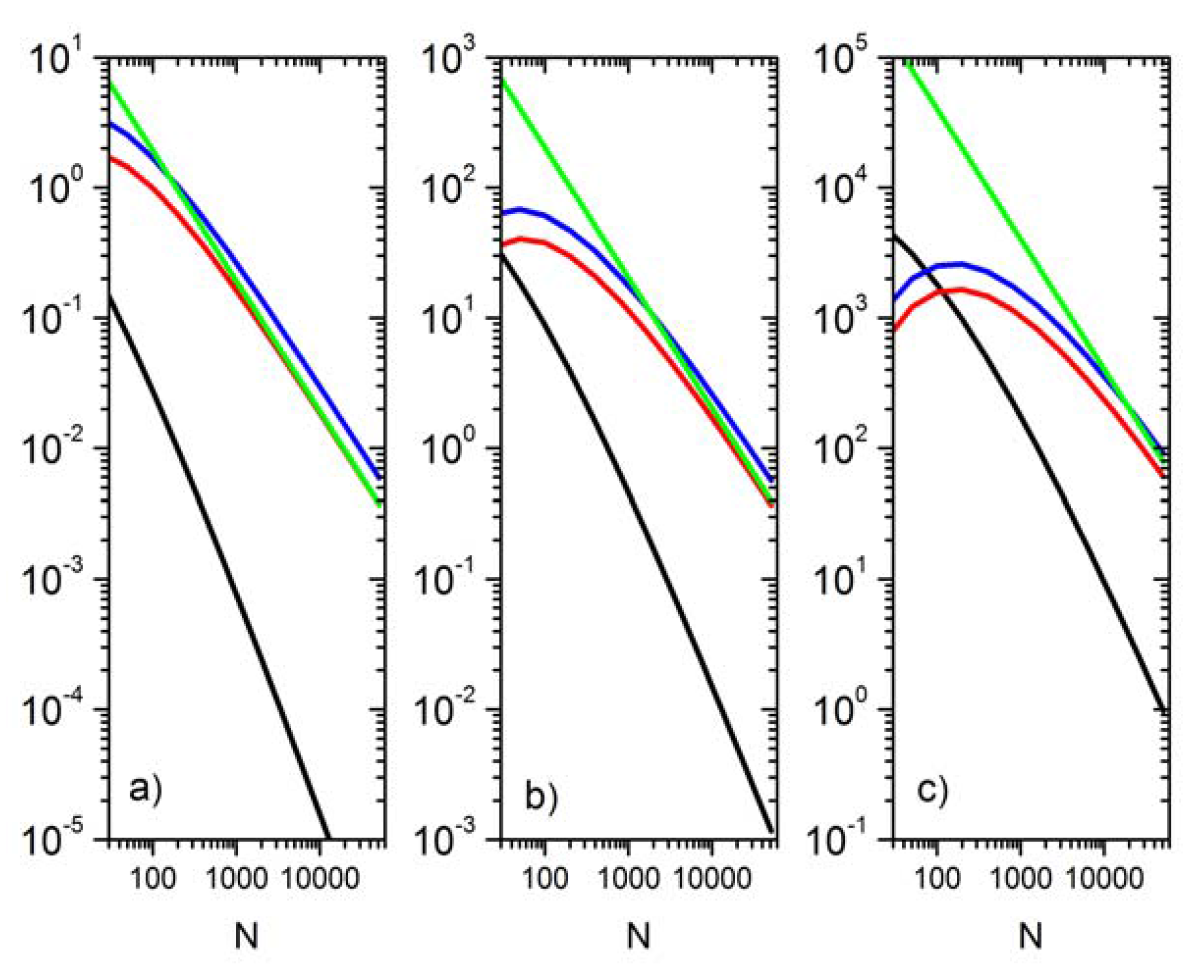
Figure 1 compares the variance $\mathrm{var}(E_N(T))$ with the squared bias ${\Vert b\Vert }^2$ of the estimator, both relevant in the bias of the MinMI estimation. In the same figure, one compares the empirical variance $\mathrm{var}(E_N(T))$, with its approximation $N^{-1}\mathrm{var}(T|lms)$ and with the variance for the case of iid trials: $N^{-1}\mathrm{var}(T)$. We use $T=X^4{Y}^2,X^6{Y}^2,X^8{Y}^2$,respectively in panels a), b), c), sorted by growing total variance $\mathrm{var}(T)$, specially concentrated at the distribution queues. In all figures, N=25*2^k,k=0,..,11. We have verified that the empirical variance $\mathrm{var}(E_N(T))$ agrees very well to the theoretical value $N^{-1}{\mathrm{var}}_N(T|lms)$ for all Ns. (not shown).

At this point, some generic conclusions can be drawn. The estimator’s variance $\mathrm{var}(E_N(T))$ grows with $\mathrm{var}(T)$ dominating over the squared bias, except for small N values and higher values of $\mathrm{var}(T)$. This will lead us to neglect the bias of covariance estimator’s in the MinMI asymptotic statistics.

Figure 1. Squared empirical bias: ${\Vert b\Vert }^2$ (black lines) of N-based $T$- expectations as function of N, empirical variances: $\mathrm{var}(E_N(T))$ (red lines), approximated variances: $N^{-1}\mathrm{var}(T|lms)$ (blue lines) and variance for the case of N iid trials: $N^{-1}\mathrm{var}(T)$ (green lines). $T$ stands for different bivariate monomials: $X^4{Y}^2$ (a), $X^6{Y}^2$ (b) and $X^8{Y}^2$ (c).

Figure 1. Squared empirical bias: ${\Vert b\Vert }^2$ (black lines) of N-based $T$- expectations as function of N, empirical variances: $\mathrm{var}(E_N(T))$ (red lines), approximated variances: $N^{-1}\mathrm{var}(T|lms)$ (blue lines) and variance for the case of N iid trials: $N^{-1}\mathrm{var}(T)$ (green lines). $T$ stands for different bivariate monomials: $X^4{Y}^2$ (a), $X^6{Y}^2$ (b) and $X^8{Y}^2$ (c).

From Figure 1, we also note that the variance reduction coming from morphisms of variables, tends to decrease for higher N values, where the effect of sampling prevails with a $N^{-1}$ scaling on the estimator variance where it is closely approximated by the asymptotic lms variance $N^{-1}\mathrm{var}(T|lms)$. That can lead to a slight increase of $\mathrm{var}(E_N(T))$ for small Ns, followed by a decrease (e.g., $X^6{Y}^2$), due to the effect that ${\mathrm{var}}_N(T|lms)$ is small for lower values of N.

Moreover, thanks to the Central Limit Theorem (CLT), the distribution of estimator errors tends towards Gaussianity with increasing N, with a slower convergence rate for higher $T$ variances. However, the Gaussian PDF limit has an infinite support which must be truncated since the estimated moments $E_N(T)$ must be within a kind of polytope with edges determined by Schwartz-like inequalities as shown by PP12 [12] (e.g., $|E_N(XY)|\le 1$ and $|E(X^{2}Y)|/{[2(1-c_g^2)]}^{1/2}\le 1)$, working as bounds for nonlinear correlations. Since estimators have bounds, the estimation errors do so as well. This can be solved by using the Fisher Z-transform arctanh(c) of a generic linear or nonlinear correlation c and projecting it over the real support (not done here).

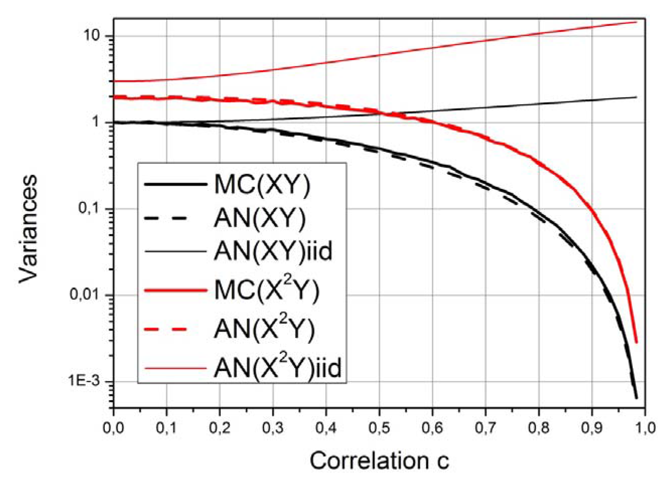
Now we illustrate in Figure 2, the Theorem 2 under different values of correlation $c_g\in [0,1]$. We consider the variables $X,Y$ with a joint Gaussian PDF of correlation $c_g\in [0,1]$ with marginal standard Gaussians. In Figure 2 we compare the empirical Monte-Carlo value of $N\mathrm{var}(E_N(T))$ (MC in the Figure), within an ensemble of 5000 N-sized samples with the theoretical one $\mathrm{var}(T|lms)$ (case where morphism is performed, AN in the Figure) and $\mathrm{var}(T)$ (case of iid realizations, ANiid in the Figure). We have used a sample of N=200, which is supposed to be near the beginning of the asymptotic regime and two cross functions: $T(X,Y)=XY$ and $T(X,Y)=X^{2}Y$. The aforementioned variances are $\mathrm{var}(XY|lms)=(1-c_g^2)/(1+c_g^2);\mathrm{var}(XY)=c_g^2+1$ while $\mathrm{var}(X^{2}Y)=12c_g^2+3$ and $\mathrm{var}(X^{2}Y|lms)$ is the mean squared residual of the best linear fit using the predictors $E(X^{2}Y|X)=c_g{X}^3$ and $E(X^{2}Y|Y)=c_g^2{Y}^3+(1-c_g^2)Y$. For both functions, a very good agreement is verified between Monte-Carlo values and the theoretical ones within 1–5% relative error. A generic result of Figure 2 is the fact that, under the fixation (presetting) of marginals, the sampling variability of cross estimators falls to zero as far the absolute value of correlation tends to one.

Figure 2. N times Monte-Carlo variances: $N\mathrm{var}(E_N(T))$ thick solid lines) and its theoretical analytical value $\mathrm{var}(T|lms)$ (thick dashed lines), both under imposed marginals (morphisms) and analytical value of $N\mathrm{var}(E_N(T))=\mathrm{var}(T)$ for iid data (thin solid lines). $T$ means different bivariate monomials: $XY$ (black curves), $X^{2}Y$ (red curves). N = 200.

Figure 2. N times Monte-Carlo variances: $N\mathrm{var}(E_N(T))$ thick solid lines) and its theoretical analytical value $\mathrm{var}(T|lms)$ (thick dashed lines), both under imposed marginals (morphisms) and analytical value of $N\mathrm{var}(E_N(T))=\mathrm{var}(T)$ for iid data (thin solid lines). $T$ means different bivariate monomials: $XY$ (black curves), $X^{2}Y$ (red curves). N = 200.

3.4. Statistical Modeling of Moment Estimation Errors

The above qualitative results gave empirical support to Theorem 2 about the covariance of estimation errors and the neglecting of estimation biases. Therefore, the part of matrix $M_{\mathrm{\Delta }{\theta }_{N,j}}$ (17) regarding cross components is modeled as:

$$M_{\mathrm{\Delta }{\theta }_{N,cr,j}}\approx N^{-1}E(E_N(T_{cr,j}{\prime }^{lms}{T}_{cr,j}{\prime }^{lms}))\equiv N^{-1}{C}_{N,cr,j|lms}$$

(30)

with the approximation being valid within terms $o(N^{-1})$. In practice, the matrix $E(T_{cr,j}{\prime }^{lms}{T}_{cr,j}{\prime }^{lms})$ requires the estimation of conditional means for each value of X and Y.

Now, we will formulate the distribution of moment’s estimation errors in the asymptotic regime of high enough N. Then, thanks to the multivariate Central Limit Theorem [34] one can suppose that the unbiased estimation error vector follows a multivariate Gaussian distribution, which is written as

$$\mathrm{\Delta }{\theta }_{N,cr,j}\approx {(M_{\mathrm{\Delta }{\theta }_{N,cr,j}})}^{1/2}{U}_j\approx N^{-1/2}{(C_{N,cr,j|lms})}^{1/2}{U}_j;U_j~N({\overrightarrow{0}}_{cr,j},P_{cr,j})$$

(31)

where ${(C_{N,cr,j|lms})}^{1/2}$ is the square root matrix of $C_{N,cr,j|lms}$ and $U_j$ is a multivariate standard normal RV of dimension equal to $\dim ({\theta }_{cr,j})$ with zero mean ${\overrightarrow{0}}_{cr,j}$ and covariance matrix $P_{cr,j}$.

4. Modeling of MinMI Estimation Errors, Their Bias, Variance and Distribution

Taking into account the Gaussian approximations (31) for estimation errors, their neglected bias, the $N^{-1}$ scaled covariance (30), and the second-order Taylor development of MinMI (9), one can determine approximated bias, variance and distribution of MinMI estimators (15).

Two problems are then addressed:

• The estimation of bias, variance, quantiles and distribution of estimators of the incremental MinMI $I_{j/p}$ issued from finite samples of N (iid) realizations of bivariate original variables $(\widehat{X},\widehat{Y})$ and then transformed into RVs $(X,Y)$
• The distribution of estimators of $I_{j/p}$ under the null hypothesis H₀ that $(X,Y)$ follows the ME distribution constrained by a weaker constraint set $(T_p,{\theta }_p)$ (j>p). These estimators work as a significance test for determining whether there is statistically significant MI beyond that explained by cross moments in $(T_p,{\theta }_p)$.

4.1. Bias, Variance, Quantiles and Distribution of MI Estimation Error

Considering the moment error distribution (31) and plugging it into the development (9), the error of the MI estimator $I_{N,j/p}$ is then distributed as:

$$\mathrm{\Delta }{I}_{N,j/p,\theta }\approx N^{-1/2}[v_{j/p}^T{(C_{N,cr,j|lms})}^{1/2}]U_j+1/2N^{-1}{U}_j^T[{(C_{N,cr,j|lms})}^{1/2}{A}_{j/p}{(C_{N,cr,j|lms})}^{1/2}]U_j$$

(32)

where neglected terms are of order $O(N^{-3/2})$. That is a second-order polynomial form of a multivariate standard Gaussian RV $U_j~N({\overrightarrow{0}}_j,P_{cr,j})$. There is no general analytical expression for the PDF inferred from (32), except in certain cases where $\mathrm{\Delta }{I}_{N,j/p}$ is a governed by a non-central Chi-squared distribution [36]. The quantiles determining the confidence intervals of $I_{N,j/p}$ can easily be obtained by sorting of Monte-Carlo surrogates (proxies) of (32) from a pseudo-random generator of a standard Gaussian. Analytical expressions of the distribution of MI estimates are given from a MI Taylor expansion in terms of the anomalies of the estimated probabilities [27,37]. Here, we adopt a different approach by considering anomalies of the estimated expectations.

The bias of $I_{N,j/p}$ or the expectation of $\mathrm{\Delta }{I}_{N,j/p,\theta }$ is derived from the mean of the quadratic form term in (32). Therefore, taking the invariance of the trace for the circular permutation of a matrix product, that bias is approximated by the asymptotic value:

$$\begin{array}{l}E(\mathrm{\Delta }{I}_{N,j/p})\approx (1/2)N^{-1}Tr(C_{N,cr,j|lms}{A}_{j/p})\\ =(1/2)N^{-1}\left[Tr(C_{N,cr,j|lms}{P}_{cr,j}{C}_{*j}^{-1}{P}_{cr,j})-Tr(C_{N,cr,p|lms}{P}_{cr,p}{C}_{*p}^{-1}{P}_{cr,p})\right]\end{array}$$

(33)

This is the difference between maximum entropy $N^{-1}$-scaled biases of orders j and p, subjected to the imposition of marginal PDFs. We must remember that if p = 0, $P_{cr,p}$ is zero. For this case the MinMI bias is simply minus the negative bias of the ME $H({\theta }_{N,j})$, which is treated without the effect of variable morphism by [26]. When data is governed by the MinMI-PDF of order j, the matrices $C_{N,cr,j|lms}$ and $P_{cr,j}{C}_{*j}^{-1}{P}_{cr,j}$ are the inverse of each-other, according to Theorems 1 and 2 (11,27), leading to $E(\mathrm{\Delta }{I}_{N,j/0})=(1/2)N^{-1}Tr(C_{N,cr,j|lms}{P}_{cr,j}{C}_{*j}^{-1}{P}_{cr,j})=(1/2)N^{-1}Tr(P_{cr,j})$, i.e., $1/(2N)$ times the number of cross constraints. However, as argued by [26], when the true data distribution is more leptokurtic than the MinMI-PDF, then the bias can be larger than $(1/2)N^{-1}Tr(P_{cr,j})$.

By assuming the limit case of Gaussianity, the variance of $\mathrm{\Delta }{I}_{N,j/p}$ comes as:

$$\mathrm{var}(\mathrm{\Delta }{I}_{N,j/p})\approx N^{-1}Tr\left[C_{N,cr,j|lms}(v_{j/p}{v}_{j/p}^T)\right]+(1/2)N^{-2}Tr\left[{(C_{N,cr,j|lms}{A}_{j/p})}^2\right]$$

(34)

The leading variance term is N⁻¹-scaled as generally deduced in [15]. Keeping the leading term of (34), and dealing with the trace, we get a given relative error $r_I=\mathrm{\Delta }{I}_{N,j}/I_j$ of the MinMI $I_{j/0}$ (p=0) when $N\ge E\left({({\lambda }_{cr,j}^T{T}_{cr,j}^{\prime })}^2\right)/{\left(I_{j/0}{r}_I\right)}^2\approx O(m_{cr,j})/{\left(I_{j/0}{r}_I\right)}^2$. The term $O(m_{cr,j})$ increases with a larger rate than $I_{j/0}$ as far as the bound of the polytope of allowed expectations is closer.

4.2. Significance Tests of MinMI Thresholds

The estimators $I_{N,j/p}$ allow for the elaboration of statistical significance tests in order to verify whether the empirical PDF differs considerably from a threshold ME-PDF or in the contrary if the difference can be justified by sampling errors.

Let us suppose the null hypothesis H₀ considering that the true PDF coincides to the ME-PDF constrained by $(T_p,{\theta }_p)$. In particular for $(T_p,{\theta }_p)=(T_{p=0},{\theta }_{p=0})=(T_{ind},{\theta }_{ind})$, the null hypothesis states that $(X,Y)$ are statistically independent. Therefore under H₀, the moment sets $(T_p,{\theta }_p),(T_j,{\theta }_j)$ are ME-congruent and the moments of order $j\ge p$ remain well determined by expectations over the less restricted p-th ME-PDF i.e., ${\theta }_j=E_{{\rho }_{T_p,{\theta }_p}^{*}}(T_j)\equiv {\theta }_{j\leftarrow p}$ where the subscript arrow $j\leftarrow p$ means that j-order statistics are obtained by the p-order ME-PDF. The same holds for the ME covariance matrices, i.e., $C_{*p}=C_p$ and $C_{*j}=C_{*j\leftarrow p}=C_j;j\ge p$. In these conditions, the matrix $C_p$ is simply a sub-matrix of $C_j$.The Lagrange multipliers are restricted to the p-order i.e. ${\lambda }_j={\lambda }_{j\leftarrow p}=({\lambda }_p,{\overrightarrow{0}}_{j/p});j\ge p$, where entries of higher order than p are set to zero leading to $v_{j/p}=0$ in (9). Therefore, the incremental MinMI vanishes, i.e. $H({\theta }_j)-H({\theta }_p)=I_{j/p}=0$, but the estimator of $I_{N,j/p}$ is positive due to artificial MI generation stemming from the presence of sampling errors. Then, under H_0, and using (9), the MI estimation is provided by the following approximation:

$$\begin{array}{l}H({\theta }_{N,p})-H({\theta }_{N,j})|H_0\equiv \delta I_{N,j/p}\approx (1/2)N^{-1}{U}_j^T[{(C_{N,cr,j|lms})}^{1/2}{A}_{j\leftarrow p}{(C_{N,cr,j|lms})}^{1/2}]U_j\\ U_j~N({\overrightarrow{0}}_j,P_{cr,j});A_{j\leftarrow p}=P_{cr,j}{(C_j)}^{-1}{P}_{cr,j}-P_{cr,p}{(C_p)}^{-1}{P}_{cr,p}\end{array}$$

(35)

where $A_{j\leftarrow p}$ is a positive semi-definite matrix. That works as a significance test for the non-verification of H₀; in other words, if $I_{N,j/p}$ is larger than an upper 1-α quantile (e.g., 1−α=95%) of $\delta I_{N,j/p}$, then H₀ is rejected with a significance level α. Those quantiles determine the significant MI thresholds and can be computed empirically as for the MinMI error (32) by a Monte-Carlo strategy. Another possibility is the fitting of the $\delta I_{N,j/p}$ distribution to a Gamma PDF with prescribed mean and variance (not done here). The bias and variance of $\delta I_{N,j/p}$ are straightforward, coming as:

$$E[\delta I_{N,j/p}]\approx (1/2)N^{-1}Tr[C_{N,cr,j|lms}{A}_{j\leftarrow p}];\mathrm{var}[\delta I_{N,j/p}]\approx (1/2)N^{-2}Tr[{(C_{N,cr,j|lms}{A}_{j\leftarrow p})}^2]$$

(36)

The N⁻²-scale for variance is also present in other MI estimate errors under the hypothesis of variable independency [27]. Under the Theorems 1 [11] and 2 [27], along with the null hypothesis, one gets $C_{N,cr,j|lms}{A}_{j\leftarrow p}=P_{cr,j}-P_{cr,p}$, thus leading to a Chi-Squared distribution for $\delta I_{N,j/p}$:

$$\delta I_{N,j/p}~(1/2)N^{-1}{\chi }_{nd}^2;\hspace{0.17em}\hspace{0.17em}nd=Tr(P_{cr,j}-P_{cr,p})$$

(37)

with $nd$ degrees of freedom, i.e., the difference between the number of cross moments of order j and p. From that, the upper quantiles necessary for statistical significance are easily obtained from χ² probability lookup tables. The bias and variance are, respectively:

$$E[\delta I_{N,j/p}]\approx (1/2)N^{-1}[Tr(P_{cr,j}-P_{cr,p})];\mathrm{var}[\delta I_{N,j/p}]\approx (1/2)N^{-2}[Tr(P_{cr,j}-P_{cr,p})]$$

(38)

By analyzing (38), and in order to get a test with a relative error $r_I=(\mathrm{\Delta }{I}_{\min }/I_{\min })$, one must choose $N\ge {\left((m_{cr2}-m_{cr1})/2\right)}^{1/2}/(I_{\min }{r}_I)$.

4.3. Significance Tests of the Gaussian and Non-Gaussian MI

In this section we particularize the theory presented in Section 4.1 and Section 4.2 (Equations 35–38) for the case of Gaussian and non-Gaussian MIs as defined in Section 2.3. For this purpose, let us consider the moment sets (13) and the MI components $I_g$ and $I_{ng,j}$ (11). Their finite estimators are:

$$\begin{array}{l}{I}_{N,g}=H({\theta }_0)-H({\theta }_{N,2})=I_g+\mathrm{\Delta }{I}_{N,g}=I_{N,j=2/p=0};\mathrm{\Delta }{I}_{N,g}=I_g(c_g+\mathrm{\Delta }{c}_{g,N})-I_g(c_g)=-\mathrm{\Delta }H({\theta }_{N,2});\\ I_{N,ng,j}=H({\theta }_{N,2})-H({\theta }_{N,j})=I_{ng,j}+\mathrm{\Delta }{I}_{N,ng,j}=I_{N,j/p=2};\mathrm{\Delta }{I}_{N,ng,j}=\mathrm{\Delta }H({\theta }_{N,2})-\mathrm{\Delta }H({\theta }_{N,j})\end{array}$$

(39)

where $\mathrm{\Delta }{I}_{N,g},\mathrm{\Delta }{I}_{N,ng,j}$ are MinMI errors, $\mathrm{\Delta }{c}_{g,N}$ is the Gaussian correlation estimation error, $H({\theta }_0)=2H_g$ with $H_g\equiv \frac{1}{2}\log (2\pi e)$ being the entropy of the univariate standard Gaussian; ${\theta }_{N,j}={\theta }_j+\mathrm{\Delta }{\theta }_{N,j};j\ge 1$ are the expectations obtained from the N-sized Gaussianized standardized sample.

The numerical implementation of the maximum entropy estimator $\widehat{H}$ (16), approximating H is computed over a number N_b bins of an extended enough finite interval [-L_i,L_i]. In the corresponding experiments (and as in PP12), we have used the calibrated values L_i=6 and N_b=80. The used algorithm is explained in detail in the appendix 2 of PP12 [12], following an adapted bivariate version of that of [35]. The error $\delta H=\widehat{H}-H$ is of the order of round-off errors, only becoming comparable to the sampling ME errors at very high values of N.

4.3.1. Error and Significance Tests of the Gaussian MI

The Gaussian MI error $\mathrm{\Delta }{I}_{N,g}$ depends on the Gaussian correlation estimation’s error $\mathrm{\Delta }{c}_{g,N}\equiv c_{g,N}-c_g$ where $c_{g,N}=E_N(XY)$ is inferred from the sample. Let us write (9) for $\mathrm{\Delta }{I}_{N,g}$. The Gaussian bivariate ME-PDF, constrained by $(T_2={(X,X^2,Y,Y^2,XY)}^T,{\theta }_2={(0,1,0,1,c_g)}^T)$ is ${\rho }_{T2,\theta 2}^{*}(X,Y)={[4{\pi }^2(1-c_g^2)]}^{-1/2}\exp [-(1/2){(1-c_g^2)}^{-1}(X^2-2c_{g}XY+Y^2)]$, leading to the vector of Lagrange multipliers ${\lambda }_2={[0,-(1/2){(1-c_g^2)}^{-1},0,-(1/2){(1-c_g^2)}^{-1},c_g{(1-c_g^2)}^{-1}]}^T$. The projector operator $P_{cr,2}$ onto cross moments is the 5x5 matrix that extracts the 5^th entry (row and column) of $T_2$, corresponding to the unique cross moment XY. The necessary 5x5 covariance matrix is $C_{*,2}=E_{{\rho }_{T2,\theta 2}^{*}}[T_2{T}_2^T]-{\theta }_2{\theta }_2^T$, where the E operator is the expectation over the bivariate Gaussian ${\rho }_{T2,\theta 2}^{*}$. Then, we apply (9) for j=2, p=0 where $\mathrm{\Delta }{\theta }_{N,j}={(0,0,0,0,\mathrm{\Delta }{c}_{g,N})}^T$. The Gaussian MI error is written in different forms as:

$$\begin{array}{l}\mathrm{\Delta }{I}_{N,g}\approx {(P_{cr,2}{\lambda }_2)}^T(\mathrm{\Delta }{c}_{g,N})+\frac{1}{2}(P_{cr,2}{C}_{*2}^{-1}{P}_{cr,2}){(\mathrm{\Delta }{c}_{g,N})}^2=\frac{c_g}{1-c_g^2}(\mathrm{\Delta }{c}_{g,N})+\frac{1+c_g^2}{2{(1-c_g^2)}^2}{(\mathrm{\Delta }{c}_{g,N})}^2=\\ =\frac{\partial I_g}{\partial c_g}\mathrm{\Delta }{c}_{g,N}+\frac{1}{2}\frac{{\partial }^2{I}_g}{\partial {c_g}^2}{(\mathrm{\Delta }{c}_{g,N})}^2\end{array}$$

(40)

There, the term $P_{cr,2}{\lambda }_2$ is the fifth component of ${\lambda }_2$, corresponding to the first derivative of $I_g$ with respect to $c_g$ whereas the term $P_{cr,2}{C}_{*2}^{-1}{P}_{cr,2}$ is the entry of $C_{*2}^{-1}$ at row 5, column 5, corresponding to the second derivative of $I_g$. The bias and variance of $\mathrm{\Delta }{I}_{N,g}$ depend on the distribution of the Gaussian correlation error $\mathrm{\Delta }{c}_{g,N}$. According to the proposed modeling of moment estimation errors (Theorem 2 of section 3.4), $\mathrm{\Delta }{c}_{g,N}$ is asymptotically Gaussian with a negligible bias $E(\mathrm{\Delta }{c}_{g,N})\approx 0$ and a variance (under imposed marginals) given by:

$$\mathrm{var}(\mathrm{\Delta }{c}_{g,N})\approx N^{-1}\mathrm{var}(XY|E(XY|X),E(XY|X))={(1-c_g^2)}^2/(1+c_g^2)$$

(41)

However, in order to keep the simulated $c_g=c_{g,N}-\mathrm{\Delta }{c}_{g,N}$ within the interval [-1,1], one can use the more precise Fisher Z-transform [38] such that $\mathrm{\Delta }{c}_{g,N}=\tanh \left({\tanh }^{-1}(c_g)+\mathrm{\Delta }{Z}_N\right)-c_g$, where $\mathrm{\Delta }{Z}_N$ has a mean and variance of order $O(N^{-1})$.

In order to test the null hypothesis that the variable pair $(X,Y)$ has a joint bivariate isotropic Gaussian distribution, we must compare the estimated $I_{N,g}$ with upper quantiles of the significance test $\delta I_{N,g}$, given by $\mathrm{\Delta }{I}_{N,g}$ (40) with $c_g=0$ and $\mathrm{\Delta }{c}_{g,N}~N(0,N^{-1})$. This is a Gaussian correlation significance test that is Chi-squared distributed, with:

$$\begin{array}{l}\delta I_{N,g}=(1/2){(\mathrm{\Delta }{c}_{g,N})}^2=(1/2)N^{-1}{U}^2~(1/2)N^{-1}{\chi }_1^2;U~N(0,1)\\ E(\delta I_{N,g})=(1/2)N^{-1};\mathrm{var}(\delta I_{N,g})=(1/2)N^{-2}\end{array}$$

(42)

4.3.2. Error and Significance Tests of the Non-Gaussian MI

The estimation error $\mathrm{\Delta }{I}_{N,ng,j}$ of the non-Gaussian MI as defined in (39) can be written as a particular form of (9) for an even order $j\ge 4$ and p=2 as function of the vector $\mathrm{\Delta }{\theta }_{N,j}$ of moment errors of the moment vector $T_j$ (13) with a certain chosen component indexation. Therefore, the matrix $A_{j/p}=A_{j/p=2}\equiv P_{cr,j}{(C_{*j})}^{-1}{P}_{cr,j}-P_{cr,2}{(C_{*2})}^{-1}{P}_{cr,2}$ of (9) comprises the inverses of covariance matrices $C_{*j}$ and $C_{*2}$, respectively of the j-th and 2^nd order ME solutions.

Algebraic consistency sets the matrix $P_2{(C_{*2})}^{-1}{P}_2$ to the embedding of ${(C_{*2})}^{-1}$ onto the j-th moment subspace. Then we will perform a range of experiments for the validation of approximations in Section 4.2. The vector $v_{j/p=2}\equiv P_{cr,j}{\lambda }_j-P_{cr,2}{\lambda }_2$ comprises Lagrange multiplier vectors of the ME solutions of orders j and 2.

In order to compute the bias, variance, quantiles and confidence intervals of $I_{N,ng,j}$, from N-sized samples, there are two possible strategies: either pure Monte-Carlo simulations or the analytical and the semi-analytical (analytical with moment’s error surrogates) approaches as explained in section 1. In the pure Monte-Carlo approach, either a known bivariate PDF is assumed or surrogates of the joint PDF are generated through multivariate bootstrapping techniques [39] preserving the copula structure. For each generated sample from an extended ensemble of N_rea (e.g., 5000) realizations, we compute moments and solve the ME problem gathering statistics afterwards. Alternatively, ME errors can be computed from the Taylor expansion (9) from moment deviations over the ensemble.

In the analytical and semi-analytical approaches, moment errors $\mathrm{\Delta }{\theta }_{N,j}$ are assumed to follow a certain parametric distribution that can be multivariate Gaussian as in (31), based on a given bias-covariance matrix modeling or a more sophisticated approach taking into account the natural bounds of the simulated moments ${\theta }_{cr,j}={\theta }_{N,cr,j}-\mathrm{\Delta }{\theta }_{N,cr,j}$. Then, MinMI statistics are computed from statistics (bias, variance, quantiles) on ensembles of error surrogates.

The non-Gaussian MIs $I_{N,ng,j}(\text{even\hspace{0.17em}\hspace{0.17em}}j\ge 4)$ work as tests measuring significant statistical deviations from the null hypotheses of joint Gaussianity. These statistical tests are given by Kullback-Leibler distances (7) and constitute an alternative to the use of algebraic deviations of moments from those given by the bivariate Gaussian (e.g., bivariate cumulants) [40].

The non-Gaussianity test of order j is given by $\delta I_{N,ng,j}\equiv H({\theta }_{N,2})-H({\theta }_{N,j})|H_0$ under the null hypothesis H₀ that the true PDF is bivariate Gaussian and is written as a particular case of (35). However, a simplification of the statistical test formula can be achieved by considering a null Gaussian correlation. This holds thanks the non-Gaussian MI invariance under variable rotations (see PP12), in particular for uncorrelated standardized variables ${(X_r,Y_r)}^T=A{(X,Y)}^T$, where A is the rotation matrix (e.g. $X_r=X,Y_r=(Y-c_{g}X){(1-c_g^2)}^{-1/2}$, i.e., the residual of the linear prediction). Under H₀, the rotated variables are still bivariate Gaussian and therefore the non-Gaussianity significance test $\delta I_{N,ng,j}$ has the same distribution as that for $c_g=0$. The matrices $C_{N,cr,j|lms}$ and $A_{j\leftarrow 2}$ entering in Equation (35) are now evaluated for Gaussian isotropic conditions. For the sake of clarity, we represent them respectively by $C_{g,N,cr,j|lms}$, $A_{g,j\leftarrow 2}=P_j{(C_{g,j})}^{-1}{P}_j-P_2{(C_{g,2})}^{-1}{P}_2$, where the subscript g stands for evaluation at ${(X,Y)}^T~N(\overrightarrow{0},I)$. For high N, $C_{g,N,cr,j|lms}=C_{g,j}$, i.e., the covariance matrix of cross j-th order moments for the isotropic Gaussian. Then we write:

$$\delta I_{N,ng,j}\approx (1/2)N^{-1}{U}_j^T\left[{(C_{g,N,cr,j|lms})}^{1/2}{A}_{g,j\leftarrow 2}{(C_{g,N,cr,j|lms})}^{1/2}\right]U_j$$

(43)

Let us specify generic entries at row α, column β of those matrices, corresponding to monomials $X^{r_{\alpha }}{Y}^{s_{\alpha }}$ and $X^{r_{\beta }}{Y}^{s_{\beta }}$ of $T_j$, i.e. with $r_{\alpha }+s_{\alpha },r_{\beta }+s_{\beta }\le j$. Then, using the notation introduced in Section 3.3 for Gaussian standard moments ${\mu }_r\equiv E(X^r);{\mu }_{N,r}\equiv E_N(X^r),r\in {\mathbb{N}}_0$, the components of $C_{g,j}$ become:

$${(C_{g,j})}_{\alpha ,\beta }={\mu }_{r_{\alpha }+r_{\beta }}{\mu }_{s_{\alpha }+s_{\beta }}-{\mu }_{r_{\alpha }}{\mu }_{r_{\beta }}{\mu }_{s_{\alpha }}{\mu }_{s_{\beta }}$$

(44)

whereas the components of the lms covariances are:

$${(C_{g,N,cr,j|lms})}_{\alpha ,\beta }={\mu }_{N,r_{\alpha }+r_{\beta }}{\mu }_{N,s_{\alpha }+s_{\beta }}-{\mu }_{N,s_{\alpha }+s_{\beta }}{\mu }_{N,r_{\alpha }}{\mu }_{N,r_{\beta }}-{\mu }_{N,r_{\alpha }+r_{\beta }}{\mu }_{N,s_{\alpha }}{\mu }_{N,s_{\beta }}+{\mu }_{N,r_{\alpha }}{\mu }_{N,r_{\beta }}{\mu }_{N,s_{\alpha }}{\mu }_{N{s}_{\beta }}$$

(45)

The bias of the non-Gaussian MinMI and its asymptotic approximation (36) are given by:

$$E[\delta I_{N,ng,j}]\approx (1/2)N^{-1}[Tr(C_{g,N,cr,j|lms}{P}_{cr,j}{C}_{g,j}^{-1})-1]=(1/2)N^{-1}\left(Tr(P_{cr,j})-1\right)$$

(46)

Similarly and following (36), the variance becomes:

$$\mathrm{var}[\delta I_{N,ng,j}]\approx (1/2)N^{-2}Tr[{(C_{g,N,cr,j|lms}{A}_{g,j\leftarrow 2})}^2]=(1/2)N^{-2}\left(Tr(P_{cr,j})-1\right)$$

(47)

and the reasonable distribution approximation following (37):

$$\delta I_{N,ng,j}~(1/2)N^{-1}{\chi }_{nd}^2;nd=Tr(P_{cr,j})-1=j(j-1)/2-1$$

(48)

from which bounds of significance levels of non-Gaussianity can be computed through quantiles of the Chi-squared distribution.

4.4. Validation of Significance Tests by Monte-Carlo Experiments

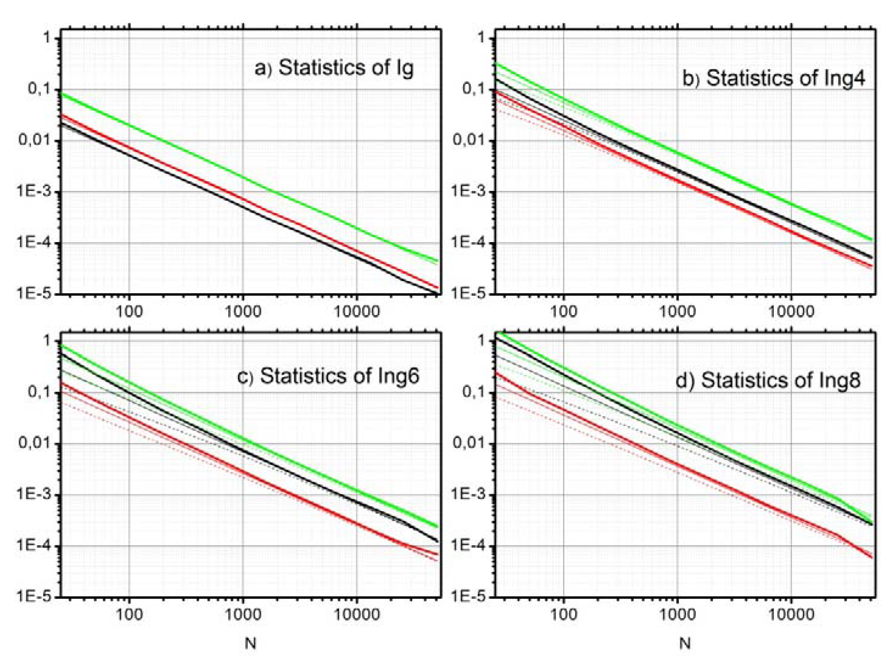
We have presented the theoretical expressions for the bias, variance and distribution, both for the Gaussian correlation test (42) and for the ME non-Gaussianity test of order j (46–48). Now we validate those expressions by comparing their results with statistics from large Monte-Carlo ensembles of ME computations. For that purpose, we have generated $N_{rea}=5000$ independent synthetic datasets of N iid uncorrelated $(X,Y)$ from a Gaussian random generator. We have set N from a duplication sequence: N=25, 2¹*25,…,2¹¹*25 = 51200. Then, we have computed the 5,000 realizations for the independency test $\delta I_{N,g}$ as well as for the non-Gaussianity tests $\delta I_{N,ng,j}$ for j = 4, 6, 8. In order to minimize errors of type $\delta H$ (8), from the ME functional, we have retained only those Monte-Carlo realizations whose ME-PDF moments are within a relative square error of 10⁻⁵.

In the sequel, we have collected and compared the estimates of bias, standard deviation and the 95%-quantile, all provided by the three approaches: the Monte-Carlo (extended ensemble of ME computations), the semi-analytical (generation of Gaussian surrogates in the Taylor expansion of ME) and the analytical (analytical formulas based on the Theorems 1 and 2). The Figure 3a, b, c and d depict the above statistics of significance tests, respectively for $\delta I_{N,g}$ and $\delta I_{N,ng,j}$ (j = 4, 6, 8). The truth is assumed to be provided by the Monte-Carlo estimate.

As previously expected, significance tests are all scaled by $N^{-1}O(1)$, and consequently their bias, standard deviation and quantiles are $N^{-1}O(1)$ as shown in Figure 3a-d by estimates coming from the different approaches. MinMI biases and significance thresholds (the 95% quantiles) grow for higher number of constraints as in the sequence $I_{N,g}$, $I_{N,ng,j=4}$, $I_{N,ng,j=6}$, $I_{N,ng,j=8}$.

These results mean that those estimators are progressively better (stronger) evaluations of MI (or the MI beyond that explained by Gaussianity), though they call for progressively higher significance thresholds. Therefore, especially in cases of under-sampled data (small N) or very low MI (or Non-Gaussian MI) values (weakly dependent variables or weak joint non-Gaussianity), there must be a tradeoff between N and the number of parameters of the MinMI estimator (here the number of cross constraints).

At this point, we discuss how the analytical and semi-analytical estimates of MinMI error statistics fit the Monte-Carlo (true) statistics. There are three crucial factors in our approximations: (1) The accuracy of the ME Taylor expansion, valid for small enough sampling errors (N large); (2) The convergence rate towards Gaussian statistics (from the CLT) for high N.

Figure 3. Test statistics: bias (black lines), standard deviation (red lines) and 95%-quantiles (green lines), provided by the Monte-Carlo approach (tick full lines), the semi-analytical approach (thin dashed lines) and the analytical approach (tick full lines). The tests are $\delta I_{N,g}$ (a); $\delta I_{N,ng,j=4}$ (b); $\delta I_{N,ng,j=6}$ (c) and $\delta I_{N,ng,j=8}$ (d).

Figure 3. Test statistics: bias (black lines), standard deviation (red lines) and 95%-quantiles (green lines), provided by the Monte-Carlo approach (tick full lines), the semi-analytical approach (thin dashed lines) and the analytical approach (tick full lines). The tests are $\delta I_{N,g}$ (a); $\delta I_{N,ng,j=4}$ (b); $\delta I_{N,ng,j=6}$ (c) and $\delta I_{N,ng,j=8}$ (d).

The analytical bias depends on factors 1 and 3, while formulas for variance, distribution and quantiles depend on all above factors, being only valid for N high enough. From Figure 3a–d, we see that the agreement between analytical and Monte-Carlo statistics is quite good for all tests (with a slight analytical underestimation), though only for large enough $N>N_{test}$ values where $N_{test}$ depends on how later (in N) the factors 1-3 hold together. We have $N_{test}\approx 50,400,1600,3200$, respectively for $\delta I_{N,g}$, $\delta I_{N,ng,j=4}$, $\delta I_{N,ng,j=6}$, $\delta I_{N,ng,j=8}$, growing with the number of constraints. The exception is when N is so large that errors $\delta H$ of the operational ME (typically, round-off errors) are of the same order of the small value tests $\delta I$, starting to influence the Monte-Carlo statistics.

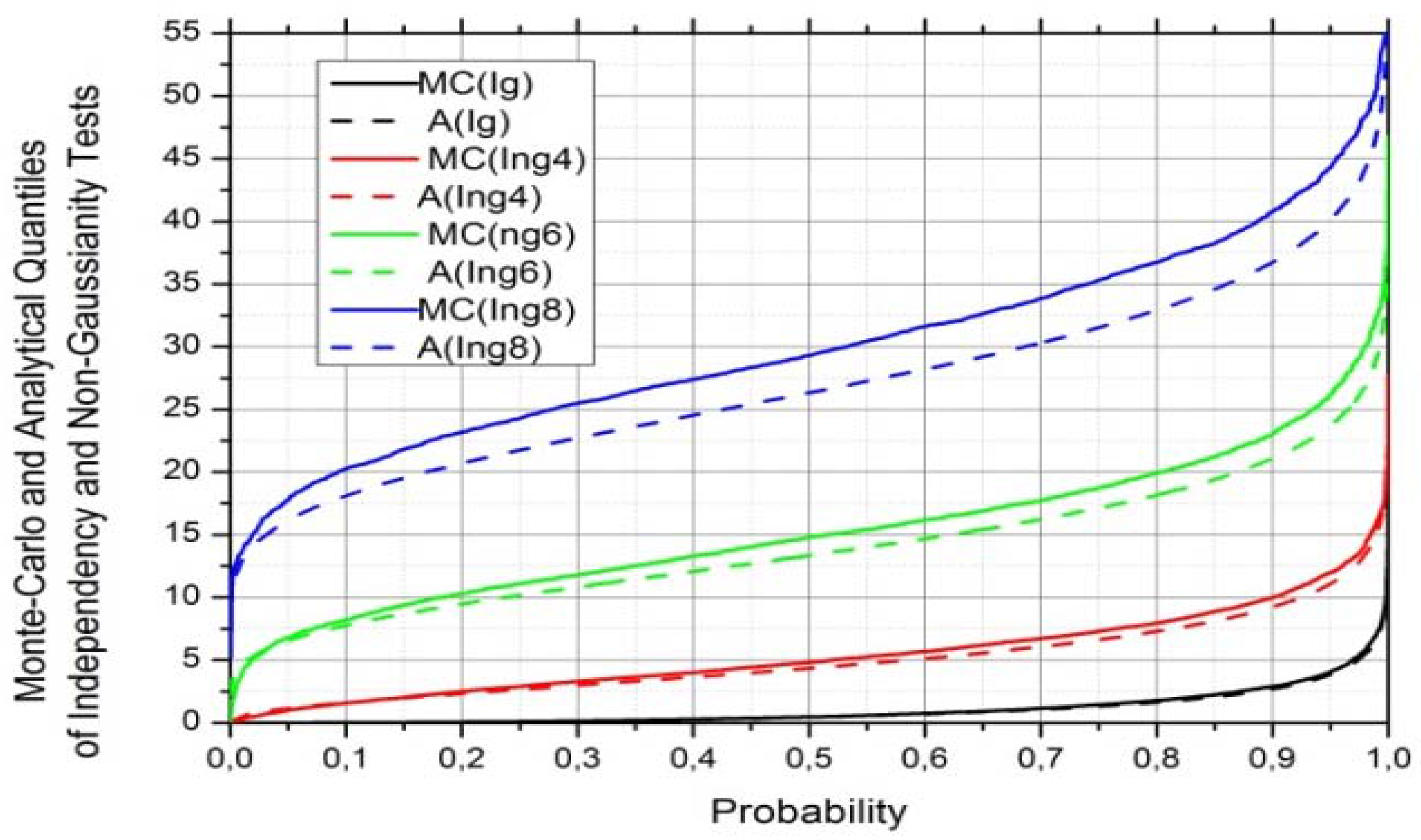
In order to validate the analytical Chi-Squared distributions for the tests, we present in Figure 4, the empirical cumulative histograms, respectively of $2N\delta I_{N,g}$, $2N\delta I_{N,ng,j}$, $2N\delta I_{N,ng,6}$, $2N\delta I_{N,ng,8}$ for $N\approx N_{test}$ and the corresponding theoretical cumulative Chi-Squared PDF fits, respectively ${\chi }_1^2$, ${\chi }_5^2$, ${\chi }_{14}^2$ and ${\chi }_{27}^2$. The agreement is shown to be quite good, with a slight deficit in the theoretical number of degrees of freedom, possibly due to uncontrolled aspects (e.g., the numerical implementation of the ME algorithm and bound effects) leading to extra randomness. In fact, the theoretical prediction of MinMI bias results from two matrices, theoretically equal, which are issued from extraordinary complicated outputs (the MinMI covariance matrix and the covariance matrix of estimators under fixed marginals). The theoretical result depends on the matching of a huge number of algorithmic details. The results provide good support to the presented Theorems, the hypotheses on the basis of the analytical and semi-analytical approaches. The slightly higher MinMI bias than the theoretical one is due to a small difference between the data PDF and the ME-PDF.

Figure 4. Monte-Carlo empirical cumulative histogram (solid lines) and theoretical cumulative Chi-Squared fit (dashed lines) normalized by N: $2N\delta I_{N,g}$ (${\chi }_1^2$) for $N=50$ (black curves); $2N\delta I_{N,ng,j=4}$ (${\chi }_5^2$) for $N=400$ (red curves); $2N\delta I_{N,ng,6}$ (${\chi }_{14}^2$) f