Abstract
A modified form of the Townsend equations for the fluctuating velocity wave vectors is applied to a laminar three-dimensional boundary-layer flow in a methane fired combustion channel flow environment. The objective of this study is to explore the applicability of a set of low dimensional, coupled, nonlinear differential equations for the prediction of possible deterministic ordered structures within a specific boundary-layer environment. Four increasing channel pressures are considered. The equations are cast into a Lorenz-type system of equations, which yields the low-dimensional set of equations. The solutions indicate the presence of several organized flow structures. Singular value decomposition of the nonlinear time series solutions indicate that nearly ninety-eight percent of the fluctuating directed kinetic energy is contained within the first four empirical modes of the decomposition. The empirical entropy computed from these results indicates that these four lowest modes are largely coherent structures with lower entropy rates. Four regions are observed: low-entropy structures over the first four modes; steep increase in entropy over three modes; steady, high entropy over seven modes; and an increase to maximum entropy over the last two modes. A measure, called the empirical exergy, characterizes the extent of directed kinetic energy produced in the nonlinear solution of the deterministic equations used to model the flow environment. The effect of increasing pressure is to produce more distinct ordered structures within the nonlinear time series solutions.
Keywords:
boundary layer flows; internal flow structures; spectral entropy rates; singular value decomposition; empirical entropy; empirical exergy PACS Codes:
05.70.Ce (entropy); 47.15.Fe (stability of boundary layers); 47.27.De (ordered regions)
1. Introduction
Significant progress has been made in recent years in the understanding of the sources of entropy production and exergy destruction in basic combustion processes. Understanding these sources of irreversibility in the combustion process should lead to improvements in thermal and combustion efficiencies of future energy conversion systems. Application of large eddy simulation (LES) techniques for the exergy analysis of turbulent combustion systems by Safari et al. [1] and the use of the direct numerical simulation (DNS) procedure in the analysis of entropy generation in turbulent premixed flames by Farron and Chakraborty [2] have clearly identified that turbulent flow conditions significantly enhance the entropy production of various physical processes within the flame structure. These studies, of necessity, assumed homogeneous turbulence environments, both upstream and downstream of the combustion process, as the bases for their studies. The existence of coherent structures within the turbulent flow environment downstream of the combustion process was not considered in these studies. The basic reason for this is that the small grid sizes required in the DNS approach to identify coherent structures together with the inclusion of all of the necessary chemical reaction effects is a daunting computing exercise.
However, application of LES techniques by Adrian [3] and the use of the DNS technique by Cherubini et al. [4] in shear flows have clearly identified coherent structures in low temperature, non combustion flow environments. The development of low-dimensional dynamical systems leading to models, which can predict these ordered structures within various flow environments, has been very successful over the past several decades. The objective for developing these models is to provide a bridge between the computation of the complicated turbulent flow environments and present computational capabilities. Lumley [5] and Holmes et al. [6] have presented the fundamental mathematical bases for the development of these low-dimensional models and applications to a number of flow environments.
The research results presented in this article are exploratory in nature with the objective of determining if such ordered structures could exist in a combustion channel downstream of a premixed combustion process. The results are presented as appropriate entropy measures for ordered structures predicted in the nonlinear time series solutions of deterministic differential equations of the Lorenz format for the combustion channel flow environment. Three measures are examined: the spectral entropy rates obtained from the power spectral density distributions in the time frame, the empirical entropy obtained from the singular value decomposition of a series of correlation matrices obtained over a series of sets of nonlinear time data along the time-dependent solution, and the corresponding empirical exergy.
The application of low-dimensional mathematical models to laminar boundary-layer flows is an active area of research [6]. The computer experiments reported here present results that indicate that such low-dimensional models may be useful in predicting local, specific regions in laminar boundary-layer flows that may be susceptible to the development of transient, ordered structures within the flow environment. No review references to the literature are included, only sources that were directly used in the development of the results are cited. This study is limited exclusively to the solutions of the low dimensional, coupled, nonlinear differential equations obtained from the Lorenz format in an assumed incompressible flow. All other considerations of stability and compressibility associated with the flow of combustion products in a combustion channel are not included.
A flow stream developing a boundary layer flow over a flat surface within a methane-fired combustion flow is taken as the environment for the study. The combustion process is assumed to consist of methane as the fuel with 300 per cent of theoretical air providing the oxidizer, with combustion completed before the combustion products enter the combustion channel flow environment. We assume an initial span wise component of velocity that yields velocity gradients in the z-y velocity plane. The resulting three-dimensional boundary layer is solved with well-established computational techniques. It has been found (Isaacson [7]) that a three-dimensional approach to the boundary layer velocity profiles is required for the prediction of ordered regions within the laminar boundary layer flow. This requirement is met by the inclusion of a flat-plate surface in the x-z plane of the flow configuration. The source code for the Keller-Cebeci Box method [8] has been implemented and serves as the computational procedure to obtain the numerical values for the velocity gradients across the boundary layers at a specific axial station from the leading edge of the flat plate surface (Isaacson [9]). Thus, similar Blasius velocity profiles (Hansen [10]) are obtained in both the x-y plane and in the z-y plane for inclusion as parameters for the computation of any velocity wave vector fluctuation that may occur within the boundary layer environment.
The Townsend equations [11] are modified into a Lorenz-type set of deterministic equations [7,9] describing the time-dependent behavior of the fluctuating velocity wave vectors of the Fourier transformed system. An internal feedback loop is included as a driver for the nonlinear transfer process between the axial fluctuating velocity wave vector and the vertical and span wise velocity wave vectors. This complete set of equations is termed the “modified Townsend equations”.
These sets of time-dependent modified Townsend nonlinear equations are solved at a specifically chosen vertical location within the three-dimensional boundary-layer structure, with the previously computed boundary layer velocity gradients at that vertical location serving as input parameters for the solution of the modified Townsend equations.
The computational solution of the modified Townsend equations yields nonlinear time series for the three velocity wave vectors for the particular vertical location within the boundary layer. For the selected values of kinematic viscosity and the vertical location within the three-dimensional boundary layer structure, these nonlinear time series solutions indicate the development of regions of aperiodic oscillatory patterns. Although only a limited number of oscillations appear in the time series (of the order of 3 to 4), the number of time steps included within this region is 4,096. Burg’s method (Chen [12] and pp. 572–575 in Press et al. [13]) is used to obtain the power spectral density for segments of limited data content over selected ranges of data within this selected time frame. Burg’s method is particularly well suited for this process, as it has the property of isolating sharp peaks in the spectral data.
The concept of spectral entropy rate production (Powell and Percival [14], Grassberger and Procaccia [15]) is used to characterize the oscillations as “disordered”, “partially-ordered”, or “ordered” regions within the nonlinear time series output. When the spectral entropy production rate for a given segment goes to zero, we classify that region of the time series as “ordered.”
The method of singular value decomposition, or proper orthogonal decomposition [5,6], Jiang and Lai [16]), has been developed and widely applied in the determination of coherent structures occurring in turbulent flows. These methods have yielded useful information concerning coherent structures resulting from the DNS of flow field structures. The method of singular value decomposition is applied to the nonlinear time-series solutions obtained from the modified Townsend equations and yields information about the coherent structures, which occur in the combustion channel flow environment. The introduction of the empirical entropy demonstrates the existence of low-entropy organized structures within the nonlinear time series solutions, together with the coexistence of partially organized structures over a narrow range of mode numbers, the existence of disorganized regions of high entropy within significant range of higher empirical modes in the nonlinear time series, and a fourth region of dissipation into maximum entropy. The introduction of the empirical exergy provides a measure for the useful energy content within the organized structures predicted in the nonlinear time series solutions of the modified Townsend equations.
The effect of raising the channel pressure for each of the entropy transfer measure is to decrease the empirical exergy in each of the respective empirical modes over the distribution of modes for the system. However, the four exergy regions that exist for the initial pressure of PR = 1.0 also exist for the pressure ratios of PR = 5.0, 10.0, and 15.0. The article concludes with a review of the results presented and observations concerning the implications of the presence of ordered structures in the computation of combustion channel flow dynamics.
2. Combustion Chamber Environment
The flow configuration that we are approximating in this exploratory study is shown in Figure 1. The combustion of methane with 100 per cent theoretical air provides the proper amount of oxygen to convert the carbon in the fuel to carbon dioxide and the hydrogen to water vapor with the nitrogen as an inert gas. This stoichiometric process provides the maximum adiabatic flame temperature. When excess air is supplied, additional oxygen and nitrogen are added to the combustion products, thus lowering the adiabatic flame temperature. Thus, the adiabatic flame temperature and the composition of the combustion products may be controlled by the amount of excess air supplied. For the study reported here, the flowing gas is made up of the products of the combustion of methane with 300 per cent theoretical air at various chamber pressures. The products of the combustion process consist of 3.38 per cent CO2, 6.77 per cent H2O, 13.53 per cent O2, and 76.32 per cent N2, with per cent by volume. The initial temperature for each case is taken as 298.15 K. The adiabatic flame temperature for these conditions is 1140.0 K. Dissociation of the products is neglected. Four cases are considered with pressures of 1, 5, 10 and 15 atm., where 1 atm. = 101.325 kPa. The transport properties for mixtures of polyatomic gases are determined by the procedures presented in Dorrance [17], including the Wilke approximation for mixtures of polyatomic gaseous species. The primary parameter required for the computation of the given set of equations is the kinematic viscosity, with the specific values determined by the applied pressure levels. The thermodynamic and transport properties used in the calculations are given in Table 1.

Table 1.
Thermodynamic and transport properties used for the computational results.
| Inlet temperature, ti | 298.15 K |
| Adiabatic flame temperature, Taft | 1140.0 K |
| Static pressure, p1 | 1.013 × 10⁵ N/m2 |
| Kinematic viscosity, ν1 | 1.523 × 10⁻⁴ m2/s |
| Static pressure, p2 | 5.066 × 10⁵ N/m2 |
| Kinematic viscosity, ν2 | 3.047 × 10⁻⁵ m2/s |
| Static pressure, p3 | 1.013 × 10⁵ N/m2 |
| Kinematic viscosity, ν3 | 1.523 × 10⁻⁵ m2/s |
| Static pressure, p4 | 1.520 × 10⁶ N/m2 |
| Kinematic viscosity, ν4 | 1.016 × 10⁻⁵ m2/s |
Figure 1.
Shown is a schematic diagram of the three-dimensional boundary-layer environment for the combustion chamber flow analysis. A Blasius boundary layer profile is also assumed in the x-y plane at the axial location x.
3. Computational Model for the Boundary-Layer Flow
The flow configuration we wish to model is the three-dimensional wall shear layer downstream of an initial starting plane, as indicated in Figure 1. For computational purposes, the free stream velocity normalizes the flow velocities and taking the surface to be a square plate 1 m in length on each side normalizes the distances. This configuration models the flow of combustion products into a flow channel with a span wise component of velocity applied to the flow at the entrance to the channel. The resulting three-dimensional boundary-layer flow environment is computed with well-established computational tools, providing the necessary input parameters for the solution of the time-dependent deterministic equations. A set of computer source codes developed for the computation of various wall shear environments has been presented in [8]. Hansen [10] has indicated that these same computational techniques may be applied to the computation of the boundary-layer velocity profiles in the span wise direction. These source codes have thus been used to create computer programs required to compute the desired three-dimensional boundary-layer flow, including the necessary gradients in the mean velocities in the three-dimensional configuration. The expressions used to calculate the gradients of the mean velocity profiles have been presented in [9].
4. Mathematical Model of the Modified Townsend Equations
The flow environment that we are considering is a low speed three-dimensional laminar boundary-layer flow near the starting plane of the flow. A specific location near the starting plane of the laminar boundary-layer flow is chosen for the computational experiment. All three x-y-z distances to this specific location in the laminar boundary layer are specified a priori. The solutions that we obtain for the derived set of low dimensional coupled, nonlinear differential equations are applicable just for this specific location. The solutions are thus local in nature and do not apply to the overall stability characteristics of the flow. The specific location chosen for the computations is significantly forward of the normal onset of transition to turbulence, with considerably reduced levels of fluctuations within the velocity fields. Hence, connections to the classical areas of stability analysis, bypass transition, or boundary-layer receptivity studies remain to be determined.
We wish to explore the behavior of a low order set of coupled, nonlinear ordinary differential equations of the Lorenz form placed in this three-dimensional shear layer environment. These equations are very sensitive to the applied initial conditions and may lead to chaotic solutions. We wish to explore the possibility that the nonlinear time series solutions of such equations may contain regions of ordered behavior. The nonlinear coupling between the various fluctuating velocity components is an essential component of the low order mathematical model of the flow environment and one of our basic objectives is to determine if such coupling leads to ordered regions within the nonlinear time series solutions.
The velocity fluctuation level within the flow is assumed to be of reduced level and homogeneous in nature. The wall is assumed to be adiabatic and the flow to be of low speed, thus allowing the assumption of incompressibility to be applied. The assumptions are made that the velocity fluctuations are nearly homogeneous in nature and that the gradients of the flow velocities obtained through the laminar boundary layer are sufficiently uniform to allow the application of Townsend’s [11] equations to this flow environment.
Using the Fourier expansion procedure as presented by Townsend [11], the equations of motion for the boundary-layer flow may be separated into steady plus fluctuating values of the velocity components. The velocity fluctuations around the mean values of the velocity components will thus be of primary interest. The equations for the velocity fluctuations may be written as follows:
In these equations, ν is the kinematic viscosity. The pressure term may be transformed as:
In these expressions, the mean velocity components are denoted by Ui, with i = 1,2,3 representing the x, y, and z components, while xj, with j = 1,2,3 denote the x, y and z directions. The three mean velocity components and the nine gradients in the mean velocities are obtained from the solutions for the boundary layer flows as outlined in [7,9].
As pointed out in [11], the pressure is determined by the velocity and temperature fields and is not a local quantity but depends on the entire field of velocity and temperature. The elimination of the pressure fluctuation term introduces nonlinear coupling between the velocity coefficients.
In our work here, we will essentially follow the procedure outlined in [9] and include an internal feedback mechanism that will model the nonlinear interaction process but will allow the resulting equations to be integrated in time. However, there are several significant modifications that we will indicate at the appropriate points.
The Navier-Stokes equations describing this flow are transformed through a Fourier analysis into a Lorenz-type format, specifically keeping the nonlinear coupling terms. The velocity fluctuations may be expanded in terms of a sum of Fourier components as:
The variation with time of each Fourier component of the fluctuation field is then given by the equation for each of the velocity wave vector amplitudes:
The equations for the rate of change of the wave numbers are:
Sagaut and Cambon [18] and Mathieu and Scott [19] have characterized the coefficients of the nonlinear velocity products in the fourth term on the right-hand side of Equation (4):
as a projection matrix, projecting any given velocity wave vector, ai, perpendicular to the direction of the corresponding wave number, ki. These authors interpret this matrix as a transfer operator for the transfer of kinetic energy occurring at low wavenumber modes, as a ‘pumping’ mechanism, toward higher wavenumber modes by nonlinear interactions.
We wish to close the set of equations, Equation (4), by replacing the projection matrix with an appropriate model equation that accomplishes the transfer process. This expression involves a coefficient of the form (1 − K ✕ cos (k(t))), with k (t) as a function of the time t. We have heuristically adopted this format for our model transfer equation. Pradeep and Hussain [20] have employed this format for small amplitude perturbations applied to a vortex column embedded in a shear flow. We have combined these elements is such a manner so that the projection matrix in Equation (4) is replaced by the expression:
K is a small, adjustable amplitude factor [20] and K(t) is the magnitude of the time-dependent axial wave number vector given by:
To simplify the nomenclature, we define F as:
The three deterministic equations for the velocity wave vectors may then be written as:
Note that the internal feedback factor is applied to the nonlinear coupling terms in the equations for and , and not to one of the directly accessible dependent variables. The application of the perturbation factor in this fashion implies that the nonlinear terms in the first-order equations for the velocity wave vector fluctuations represent a “pumping” process, transferring energy from the axial velocity wave vector, ax, into the vertical velocity wave vector, ay, and the span wise velocity wave vector, az.
The set of equations for the time-dependent wave numbers is obtained by including the gradients of the mean velocities in the x-y and z-y boundary layers as follows:
With these approximations, we uncouple the continuity equations for the wave numbers from the solutions of the nonlinear deterministic equations for the velocity fluctuation wave vectors. The equations for the fluctuating velocity components have thus been transformed into a form similar to Lorenz-type equations, as shown by Hellberg and Orszag [21] and Isaacson [22]. The values of the mean velocity gradients as determined by the solution of the boundary-layer flows, the gas mixture kinematic viscosity and an amplitude factor accounting for the degree of internal feedback included in the nonlinear coupling terms in the modified Townsend equations are the significant parameters required for the solution of the resulting set of six simultaneous equations. Our objective is to explore the particular laminar three-dimensional boundary layer for any particular set of these parameters which yields a nonlinear time series solution of these modified Townsend equations that may contain ordered regions within the solution. We then introduce various entropy measures that describe these ordered regions within the output time series solution.
In our initial studies, it was found that three equations of the Lorenz type were required for the solutions to exhibit combinations of ordered and disordered regions. This required the inclusion of the equation for the span wise wave number vector and the equation for the fluctuating span wise velocity wave vector. The flat plate surface in the x-z plane was added to the flow model to provide the boundary layer in the z-y plane for the necessary velocity gradients required in the additional equations. The velocity gradients in the z-y plane are obtained from the solution of the boundary-layer equations for the Blasius boundary-layer flow in the z-y-plane. It has also been found that the flat plate surface in the x-z plane must be small, of the order of z = 0.003 in width, for the overall solutions to exhibit ordered and disordered regions. These observations have led to the fairly complicated three-dimensional flow model adopted in this study. Corresponding results have not been found for two-dimensional boundary-layer flows.
The choice for the initial axial distance (distance in the x-direction) for the computation of the boundary-layer profiles was made to compare the results of the computed boundary-layer profiles with previously published results [8]. It has also been shown previously [7] that boundary-layer ordered fluctuating velocity wave vectors are primarily initiated within the wall shear layer at the vertical station of j = 16. These considerations then lead us to a particular location for the computations of the nonlinear time series solutions of the modified Townsend equations.
The theoretical modeling of the fluctuating velocity components within the boundary-layer flow consists of six simultaneous first-order differential equations, solved at the vertical station of j = 16 within the wall shear layer. The solution of this set of equations yields the velocity-fluctuation wave-vectors in three-dimensions for this particular vertical station at the axial station of nx = 4 (x = 0.08), the span wise station of nz = 4 (z = 0.003), and the value of the vertical location yxz = 0.004 of the z-y plane boundary-layer surface. This location of the x-z surface brings the similar Blasius velocity gradient profile in the z-y plane into proper alignment with the similar Blasius profile in the x-y plane.
The equations are integrated using a fifth-order Runge-Kutta technique with computer source codes as presented on pp. 714–720 in [13]. First, the three first-order differential equations for the wave numbers are integrated in time with the resulting series stored to files on the hard drive. A time step of 0.0001 s is used with a total of 12,288 time steps included in the integration process. The nonlinear time series solution diverges rapidly beyond the time step of n = 12,288 (see [6]). Hence, the integration process is terminated at this point. These stored data files thus become available for the solution of the time-dependent deterministic equations for the fluctuating velocity wave vectors. The resulting axial velocity wave vector (we define the velocity wave vector in the x-direction as the axial velocity wave vector) nonlinear time series signal is then processed to characterize the signal within the various regions and to compute the three entropy measures within those regions.
Figure 2 presents the variation of the fluctuating axial velocity wave vector as a function of the time step. These results indicate that after a period of induction, aperiodic oscillatory large-scale patterns develop in the fluctuating axial velocity wave vector. The axial velocity wave vector is plotted in Figure 2 and Figure 4, Figure 5 and Figure 6 as a function of the time step of the time integration process for comparison with the computational techniques introduced later in the article for the evaluation of the several entropy measures.
Figure 2.
The axial velocity wave component ax from the modified Townsend equations is shown as a function of the time step, n. Parameters: Taft = 1140.0 K, PR = 1.0, x = 0.08, z = 0.003, j = 16 (η = 3.0).
The three-dimensional representation of the fluctuating velocity wave vector trajectories produced by the modified Lorenz system of equations is shown in Figure 3. The familiar saddle-shaped phase space trajectory of the Lorenz system of equations is readily apparent in this figure.
Figure 4 shows the axial velocity wave component ax from the modified Townsend equations as a function of the time step for a channel pressure ratio PR = 5.0. The effect of increasing pressure is apparent in the decrease in the number of large-scale aperiodic cycles represented in the nonlinear time series solution.
Figure 3.
The three-dimensional representation of the fluctuating velocity wave vector trajectories produced by the modified Townsend equations is shown. Parameters: Taft = 1140.0 K, PR = 1.0, x = 0.08, z = 0.003, j = 16 (η = 3.0).
Figure 4.
The axial velocity wave component ax from the modified Townsend equations is shown as a function of the time step, n. Parameters: Τaft = 1140.0 K, PR = 5.0, x = 0.08, z = 0.003, j = 16 (η = 3.0).
Figure 5 and Figure 6 show the axial velocity wave vector ax from the modified Townsend equations for chamber pressure ratios of PR = 10.0 and PR = 15.0 as a function of the time step. The results presented in Figure 4, Figure 5 and Figure 6 indicate that increasing the combustion channel pressure does not eliminate the generation of aperiodic structures within the wall shear layer, and that these structures may be produced in the channel as the pressure is increased into the operational range. It therefore becomes necessary to a gain a better understanding of the nature of these structures and to delineate the ordered activity within the structures. The spectral entropy as discussed in the next section is introduced to provide additional information concerning the nature of the ordered activity within these structures.
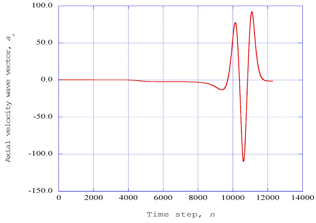
Figure 5.
The axial velocity wave component ax from the modified Townsend equations is shown as a function of the time step, n. Parameters: Taft = 1140.0 K, PR = 10.0, x = 0.08, z = 0.003, j = 16 (η = 3.0).
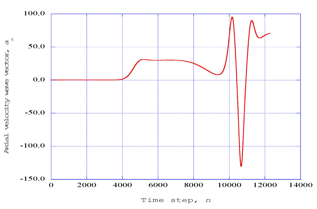
Figure 6.
The axial velocity wave component ax from the modified Townsend equations is shown as a function of the time step, n. Parameters: Taft = 1140.0 K, PR = 15.0, x = 0.08, z = 0.003, j = 16 (η = 3.0).
5. Prediction of Spectral Entropy Rates from the Deterministic Results
The results from the time integration of the modified Townsend equations consist of nonlinear time series outputs for the each of the wave number vectors and for the three fluctuating velocity wave vectors. The results presented in Figure 2, Figure 3, Figure 4, Figure 5 and Figure 6 indicate the prediction of large-scale aperiodic oscillatory patterns in the flow behavior after a time step of 8192. However, we are interested in the fine-scale structure of the nonlinear time series of data within these aperiodic oscillatory patterns. Obtaining an understanding of the fine-scale behavior requires a study of selected sets of data within the time series output. We have used Burg’s method to obtain the power spectral density within selected data sets over the range of time steps indicating the large-scale patterns. A significant advantage of Burg’s method is the enhancement of the spectral peaks in the power spectral density distribution. Our previous experience with Burg’s method [7,9] and the existence of useful source codes for the analysis of the predicted time series led to our use of this method for the evaluation of the power spectral density of the axial velocity wave vector, ax, for each data segment in the time series.
The application of the Fourier transform, Equation (3), to the equations for the fluctuating velocity vectors yields a set of low-order time-dependent deterministic equations for the wave numbers and for the fluctuating velocity wave vectors. The results presented thus far have been concerned with the behavior of the wave numbers and the individual velocity wave vectors as a function of the integration time step. However, we are interested in the behavior of the actual physical fluctuating velocity vectors and to obtain an entropy measure associated with these actual velocity vectors.
To accomplish this extension to the physical plane, we note a very useful property of the Fourier transform in that the norm of the velocity wave vectors as computed from the deterministic equations is equal to the norm of the actual fluctuating velocity vectors through Parseval’s formula (Papoulis [23], Thomas [24]). We, therefore assert, that the power spectral density obtained from the nonlinear time series solution of the modified Townsend deterministic equations for the velocity wave vectors also represents the power spectral density of the time-dependent nonlinear time series for the physical velocity vectors. Thus, the spectral entropy rates obtained in this section are applicable to the spectral entropy rates associated with the various ordered and disordered regions contained within the nonlinear time series solutions of the modified Townsend deterministic equations.
We are interested in the detailed structural characteristics of the nonlinear time series output during the time period of the production of the large-scale patterns. From previous studies [7], the time-dependent internal feedback parameter, F, begins to deviate from its initial value between time steps of 6000 and 8000. As time-dependent control parameters in the modified Townsend equations, variations of the wave numbers will affect the computational output within the overall solutions. Thus, we have selected the time step of n = 8192 as the initial point for the computation of the spectral entropy rates within the nonlinear time series output.
The method of computation used for the prediction of the distribution of the power spectral density rate is the maximum entropy method (Burg’s method) presented by Press et al. pp. 572–575 in [13]. The power spectral density for the axial velocity wave vector time series is computed for 4096 time step data samples from time step of n = 8192 to time step n = 12,288. The selected time series is divided into 128 segments with 32 data sets per segment. Burg’s method (pp. 572–575 in [13]) is applied to each segment of the 128 data sets to obtain 64 spiked values of the power spectral density of the axial velocity wave vector, fr, for each particular segment. The procedure is much like a boxcar averager, with a window of 32 data values each, with the window proceeding from the initiation of the calculations through 128 frames to the end of the overall data set. Thus, at a fixed point in physical space, we are evaluating the spectral entropy rate content of each succeeding 32 data points proceeding over 128 frames in temporal space.
The spectral entropy rate evaluated from the power spectral density is used as a measure of the degree of order within each specific segment of the nonlinear time series obtained from the solution of the modified Townsend equations for the fluctuating axial velocity wave vector. The probability value for the particular power spectral density for a given time segment is first computed from .
The methods of [14,15] are then applied to the probability distributions for each time segment to develop the spectral entropy rate for the given segment. The spectral entropy rate (1/s) is then defined for the j-th time segment as:
The spectral entropy rate results for the modified Townsend system of equations are presented in Figure 7, Figure 8, Figure 9 and Figure 10 for the pressure rations of 1.0, 5.0, 10.0 and 15.0. These spectral entropy rates are computed from 128 time data segments covering the block of nonlinear time series output from the time step of n = 8192 to the time step of n = 12,288 at the vertical boundary-layer stations of j = 16 (η = 3.00) and for the span wise station nz = 4(z = 0.003) at the axial station of nx = 4 (x = 0.08). The spectral entropy rate for a given segment reflects the nature of the data elements within that segment as to whether they are “regular” or “irregular” [14]. Thus, spectral entropy rates only have meaning when they are associated with a grouping of data elements, and not for individual time data elements. The results indicate a significant level of chaotic behavior of high spectral entropy rates (~0.35), interspersed with intermediate regions of lowered spectral entropy rates (~0.20). The important observation, however, is that several downward spikes of spectral entropy rates to zero value indicate the production of ordered structures within the axial velocity wave vector time segments.
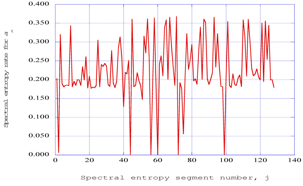
Figure 7.
The spectral entropy rate presented as a function of the segment number for the axial velocity wave vector, ax output from the modified Townsend equations. Parameters: Taft = 1140.0 K, PR = 1.0, x = 0.08, z = 0.003, j = 16 (η = 3.00).
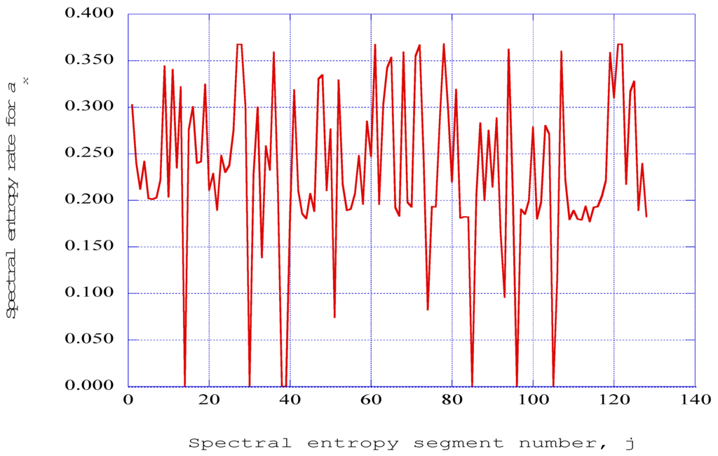
Figure 8.
The spectral entropy rate presented as a function of the segment number for the axial velocity wave vector, ax output from the modified Townsend equations. Parameters: Taft = 1140.0 K, PR = 5.0, x = 0.08, z = 0.003, j = 16 (η = 3.00).
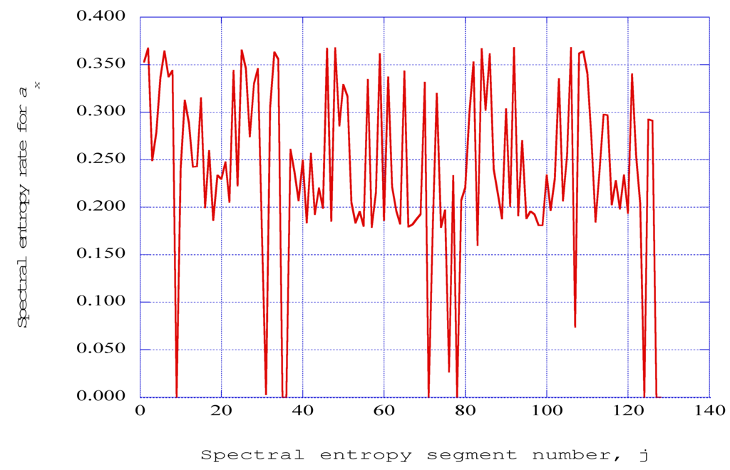
Figure 9.
The spectral entropy rate presented as a function of the segment number for the axial velocity wave vector, ax output from the modified Townsend equations. Parameters: Taft = 1140.0 K, PR = 10.0, x = 0.08, z = 0.003, j = 16 (η = 3.00).
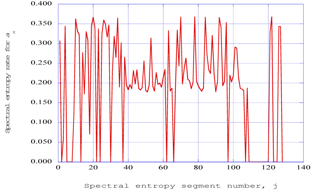
Figure 10.
The spectral entropy rate presented as a function of the segment number for the axial velocity wave vector, ax output from the modified Townsend equations. Parameters: Taft = 1140.0 K, PR = 15.0, x = 0.08, z = 0.003, j = 16 (η = 3.00).
Thus, for the selected location in the boundary-layer spatial coordinates, and for the particular values of amplitude parameter and the initial conditions, the initial computational results for the modified Townsend equation system indicate a time-dependent transition process between ordered, partially ordered, and chaotic states. The spectral entropy is a measure of how concentrated or widespread the ordered structure is within the flow environment. For a channel pressure of PR = 1.0, Figure 7 indicates that the spectral entropy rate goes to zero over a fairly wide range of segment data. As the channel pressure is increased, Figure 8, Figure 9 and Figure 10 indicate that the spectral entropy rates become more concentrated, with closer groupings of zero rates earlier in the data segment number range. The singular value decomposition procedure, as presented in the next section, will provide a clearer understanding of the characteristics of each of these structures and will introduce measures that will quantify these characteristics.
6. Singular Value Decomposition, Empirical Entropy and Empirical Exergy
6.1. Introduction to the Application of the Singular Value Decomposition Method
The spectral entropy rates as computed in the previous section provide an indication that the nonlinear time series solution of the deterministic equations for the fluctuating velocity wave vectors develops ordered structures sequentially within the time series data. It would be of interest to gain information about the temporal structures that are formed within the time series. The method of singular value decomposition, or proper orthogonal decomposition (Lumley [5], Holmes et al. [6], Jiang and Lai [16]), has been developed and widely applied in the determination of coherent structures occurring in turbulent flows. These methods have yielded useful information concerning coherent structures resulting from the DNS of flow field structure. The principle of proper orthogonal decomposition (POD) is the decomposition of the flow field into a weighted linear sum of orthogonal eigenfunctions [16], or as indicated by Holmes et al. [6], sometimes called empirical eigenfunctions, or POD modes. The application of the singular value decomposition procedure (or POD) yields eigenvalues λj that represent twice the value of the kinetic energy in each of the modes . Holmes et al. [6] called these eigenvalues empirical eigenvalues. We will use the term “singular value decomposition procedure” in our presentation because we have used the source code presented by Press et al. (pp. 59–70 in [13]) under this classification.
We have applied the singular value decomposition procedure to the nonlinear time-series solution of the modified Townsend deterministic equations resulting from the Fourier transform of the original Townsend equations. Again, invoking Parseval’s formula [23,24], we assert that the empirical eigenvalues produced by the singular value decomposition procedure represents twice the kinetic energy associated with the fluctuating velocity fields in addition to the fluctuating velocity wave vector fields.
In a similar treatment from information theory and stochastic complexity, Rissanen [25] introduces a term he calls the empirical entropy, Sempj, defined by the expression:
where λj is the empirical eigenvalue computed from the singular value decomposition procedure applied to the nonlinear time-series solution.
We characterize the term, Sempj, as the empirical entropy associated with the eigenvalue λj for the empirical mode j. The empirical entropy of the mode j is associated with the decrease of order within the directed kinetic energy of the fluctuating velocity component over the particular time frame associated with the correlation procedure and the singular value decomposition computation. This decrease in directed kinetic energy is inherent within the solution of the deterministic equations and is apparently not a result of the decay of higher ordered modes.
The first four modes of the decomposition process contain nearly ninety-eight percent of the fluctuating kinetic energy. The lowest mode has essentially negligible empirical entropy, and hence has the potential for maximum conversion into external work without external irreversibility. To define a measure for this potential, we introduce the term thermo mechanical availability or empirical exergy of that state relative to the system dead state (Wark [26]). We define the empirical exergy Eempj by the expression:
This measure will indicate the degree of “order” within the “empirical mode, j” of the deterministic structure over the selected time range of the nonlinear time series output of the computations. Note that the static pressure level of the particular state is not included in this definition of empirical exergy.
6.2. Computational Procedures for the Empirical Entropy and the Empirical Exergy
We wish to present the computational procedures in detail for two fundamental reasons. First, clearly identifying the computational procedures should lead to a better understanding concerning the fundamental significance of each of these measures in characterizing the nature of deterministic structures predicted from low-order time-dependent deterministic models of the fluctuating flow. Second, possible errors in the theoretical fundamentals or in the computational procedures may be identified and corrected in future work.
The first computational process is to determine the autocorrelation of the fluctuating axial velocity wave vectors over the time frame of a selected data set. The correlation source code presented by Press et al. (pp. 545–546 in [13]) is used to prepare the required matrix for processing by the singular value decomposition procedure. A data set of 1024 time data values is separated into 16 sequential windows. Each window allows 64 normalized data values into the correlation process. The correlation process produces 16 output values from the 64 input data values. These 16 correlation output values for each window are then normalized by the maximum in each individual set of 16 values. This process provides an input 16 × 16 matrix of 16 normalized autocorrelation values in each of the 16 sequential windows in the time series data. Application of the singular value decomposition computational procedure (Press et al. pp. 59–70 in [13]) to this matrix then yields the empirical eigenvalues for each of the empirical eigenfunctions for the time frame covering the 1024 chosen time steps.
Figure 11 presents the sum of the fraction of kinetic energy contained within each empirical eigenmode over the range of modes from 1 to 16. It is apparent that close to ninety-nine percent of the directed kinetic energy within the system is contained within the first four eigenmodes. Thus, these four modes represent highly ordered structures. The empirical entropy measure presented in Figure 12 verifies the highly organized nature of these four modes for each of the applied pressure ratios. In addition, the results indicated in Figure 12 bring to light four distinct regions within the nonlinear time series. The first region is the highly organized structure of the first four modes. The second region is the steep increase in empirical entropy over modes five, six and seven, indicating a possible phase transition. The third region is an almost uniform region of high empirical entropy of disorganized structures over modes eight through fourteen. The final region, from modes fifteen to sixteen, indicates a region of maximum empirical entropy.
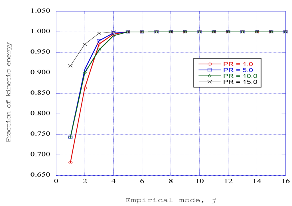
Figure 11.
The sum of the fraction of kinetic energy over the empirical mode numbers for each of the chamber pressure ratios. Parameters: Taft = 1140.0 K, x = 0.08, z = 0.003, j = 16 (η = 3.00).
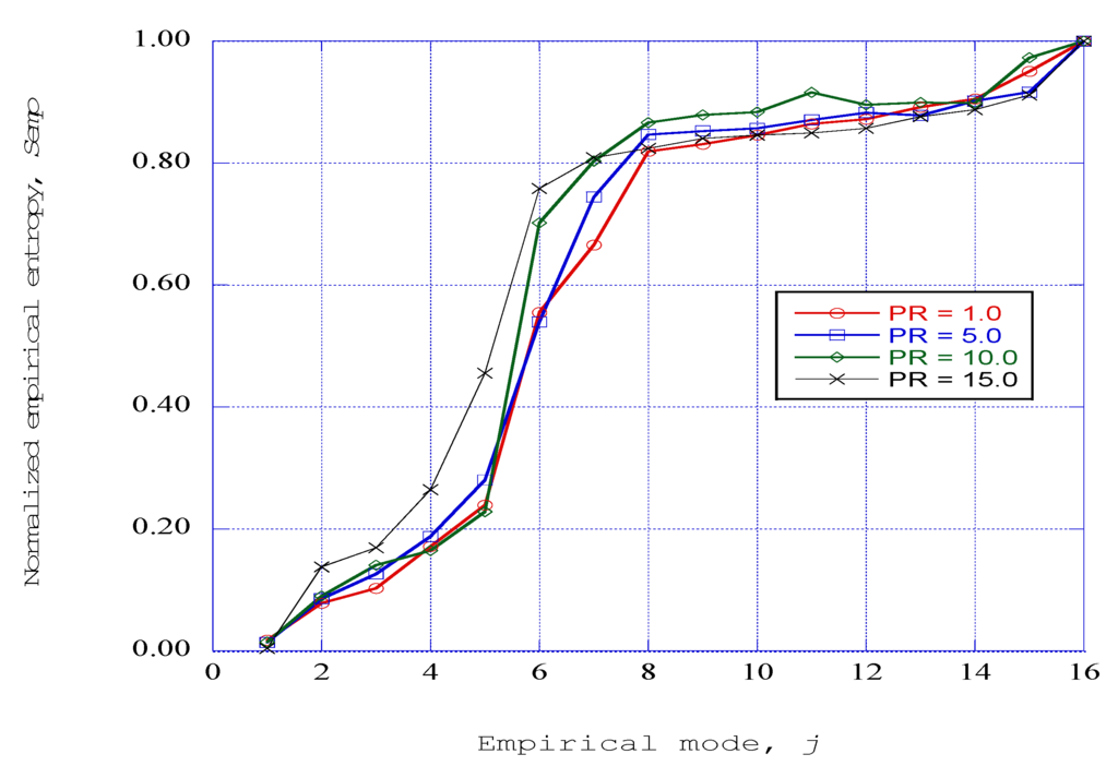
Figure 12.
The normalized empirical entropy over the empirical mode numbers for each of the chamber pressure ratios. Parameters: Taft = 1140.0 K, x = 0.08, z = 0.003, j = 16 (η = 3.00).
The normalized empirical exergy as a function of the empirical mode number for a channel pressure ratio of 1.0 is shown in Figure 13. Here, the four regions identified by the empirical entropy over the nonlinear time series are clearly identified. Logarithmic curve fit equations are given in this figure for each of the four identified regions. These expressions may be helpful in studies directed at evaluating the loss of exergy within similar energy producing flow systems.
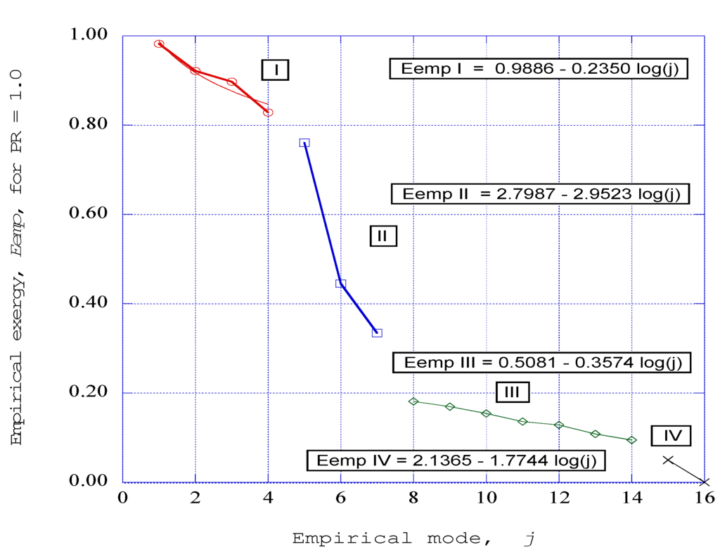
Figure 13.
The normalized empirical exergy over the empirical mode numbers for a chamber pressure ratio, PR = 1.0. Parameters: Taft = 1140.0 K, x = 0.08, z = 0.003, j = 16 (η = 3.00).
Figure 14 presents the empirical exergy as a function of empirical mode number for each of the channel pressure ratios considered in this study. The effect of increasing the operating pressure within the channel is to increase the loss of exergy from the ordered structures in the first four empirical modes. The steep loss of exergy begins at the third mode and extends over modes four, five, and six. The third region of disorganized structures with low exergy is spread over a wide range of mode numbers from seven to fifteen, with dissipation of remaining exergy to zero at mode sixteen.
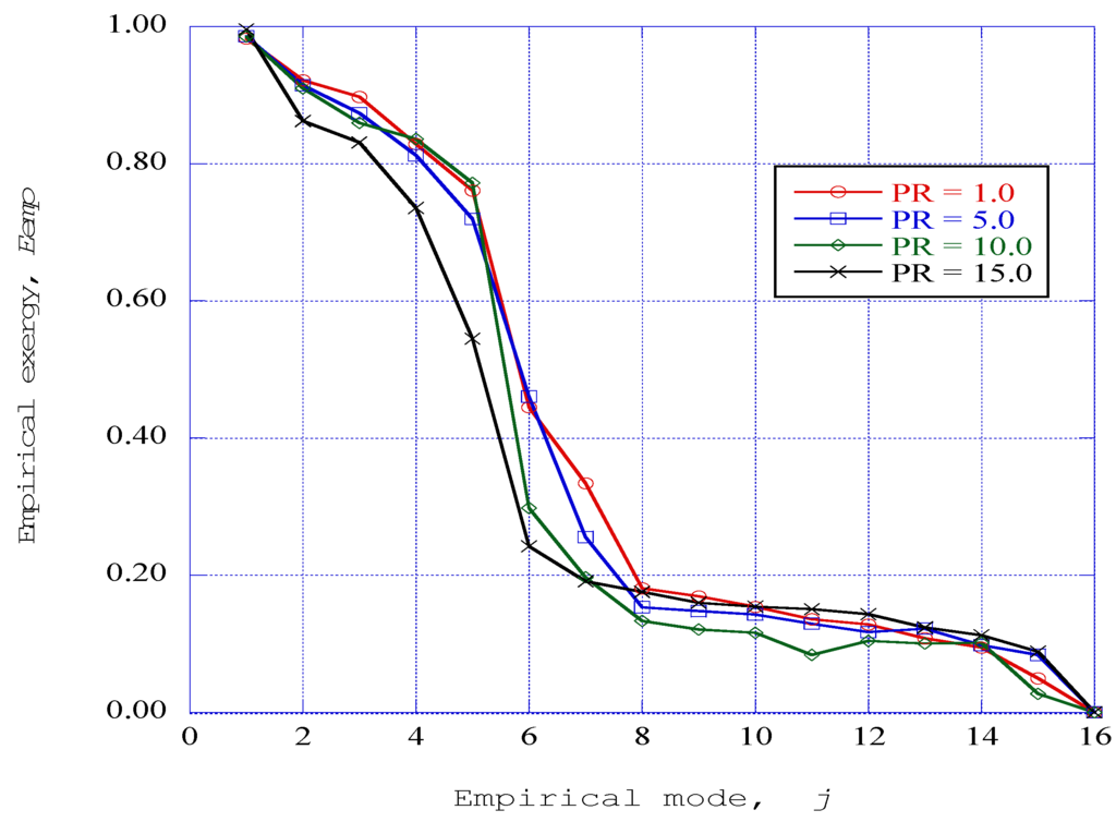
Figure 14.
The normalized empirical exergy over the empirical mode numbers for each chamber pressure ratio. Parameters: Taft = 1140.0 K, x = 0.08, z = 0.003, j = 16 (η = 3.00).
7. Discussion
The fundamental objective of this exploratory study has been to gain a better understanding of the nature of deterministic structures predicted by modified Townsend equations applied to a three-dimensional laminar boundary layer at the entrance to a combustion channel fired by the products of a methane-fueled combustion process. Three entropy-related measures have been computed from the nonlinear time series solution of the Lorenz form of the modified Townsend equations. These entropy measures have been computed for four pressure levels within the combustion channel.
The first measure, the spectral entropy rate, has been computed over a sequence of time-data segments of the nonlinear time series results of the time integration of the modified Townsend equations. For the initial pressure level within the combustion channel, (PR = 1.0), the spectral entropy rates indicate the presence of regions of organized structure, with spectral entropy rates of zero at several interior segments of the process. Also included in the results are regions of partially ordered structures and regions of disorganized structures.
As the pressure level within the combustion channel is raised, the number of segments in which the spectral entropy rates which go to zero increases, with the indication of ordered structures occurring earlier in the time integration process. At the maximum pressure level considered (PR = 15.0), the spectral entropy rates presented in Figure 10 indicate the clustering of ordered structures in the earliest spectral entropy segment numbers. Thus, the effect of increasing the pressure is to bring about a consolidation of the ordered structures into a more compact form.
The second entropy measure examined, the empirical entropy, has been computed through the use of the singular value decomposition method. The singular value decomposition computational method yields a set of empirical eigenfunctions (empirical modes) over which the directed kinetic energy of the fluctuating axial velocity field is distributed. The resulting normalized empirical eigenvalues then represent the fraction of the kinetic energy that resides in each of the empirical modes. For the initial pressure (PR = 1.0) within the combustion channel, the fraction of kinetic energy in the first mode is of the order of sixty-eight percent. Over ninety-eight percent of the kinetic energy resides in the first four empirical modes of the decomposition.
As the pressure level is raised to the maximum considered in this study (PR = 15.0), the fraction of kinetic energy in the first mode increases to a level of approximately ninety-two percent. Again, the first four modes of the decomposition contain nearly ninety-nine percent of the kinetic energy in the system.
The empirical entropy is computed from the distribution of eigenvalues. The first four empirical modes, which contain the majority of the kinetic energy, show a very low level of empirical entropy, slightly increasing from the first mode to the fourth mode. Then there is a steep increase in empirical entropy over modes five, six, and seven, which represents a significant increase of disorder within these regions within the nonlinear time series solution of the modified Townsend equations. The empirical entropy is approximately constant over empirical modes eight through fourteen, apparently representing the existence of disordered structures in this range. Finally, from mode fifteen to sixteen, there is an abrupt increase to maximum empirical entropy, apparently indicating the complete “dissipation” of kinetic energy.
The effect of raising the channel pressure is to increase the empirical entropy in each of the respective empirical modes over the distribution of modes for the system. The four entropy regions shown for the initial pressure of PR = 1.0 also exist for the pressure ratios of PR = 5.0, 10.0, and 15.0.
The introduction of the empirical exergy, or availability, provides a measure of the order within a particular empirical mode obtained from the singular value decomposition computation. With the maximum fraction of kinetic energy in the first empirical mode, the empirical exergy for that mode is approximately unity. The exergy for the first four modes indicates a slightly decreasing value from the maximum value. This is to be expected from the observation that nearly ninety-nine percent of the kinetic energy resides in these four modes. Then, for modes five, six, and seven, there is a steep decrease in exergy. These regions coexist with the first four, ordered regions, and may represent the presence of a “sheath” type of structure [20] surrounding the ordered structures. This observation clearly is speculation and this question needs to be resolved. The third region in the representation of exergy is the existence of low exergy structures across modes eight through fourteen. Finally, the exergy decreases to zero at mode sixteen.
The effect of raising the channel pressure is to decrease the empirical exergy in each of the respective empirical modes over the distribution of modes for the system. However, the four exergy regions that exist for the initial pressure of PR = 1.0 also exist for the pressure ratios of PR = 5.0, 10.0, and 15.0.
The demonstration that the primary structures within the system consist of the first four empirical modes of the singular value decomposition computation provides a proper basis for the consideration of the low-dimensional model represented by the modified Townsend equations (Holmes, et al. [6]). In addition, it should be noted that the range of kinematic viscosities covered by the composition of the combustion products, the adiabatic flame temperature, and the range of applied pressure ratios is significant. Since the value of the kinematic viscosity is a key parameter in the overall solution of the modified Townsend equations, we should anticipate that other applications, which have kinematic viscosity in this range, might also exhibit these types of structures.
The primary objective of this study has been to explore the possibility that certain laminar boundary layers may encounter conditions that may lead to the initiation of time-dependent ordered structures. We have delineated specific conditions within a combustion channel that exhibit such time-dependent ordered structures for various pressure levels within the channel. We should not anticipate that our results would be directly applicable to the computation of entropy within such channels. Rather, a better understanding of the time-dependent flow dynamics within the channel may lead to more accurate dynamic numerical simulations which then should provide more accurate design information for operational systems. Our studies are being extended to the application of the modified Townsend equations in other flow environments and configurations and very interesting results are being obtained. These results will be reported in future publications.
We should note that the modified Townsend equations, as cast in this study, are a very quirky set of equations. As is true for Lorenz-type nonlinear equations in general, the solutions for these equations are highly sensitive to the initial conditions applied to the equations. In addition, the computations are sensitive to the values for the kinematic viscosity and the weighting factor. Considerable persistence and patience are required to obtain consistent solutions.
8. Conclusions
A set of low dimensional, coupled, nonlinear differential equations in the Lorenz format have been solved for a three-dimensional Blasius boundary layer flow in a combustion products environment. The Townsend equations for the fluctuating velocity components have been Fourier-transformed into a set of six ordinary coupled differential equations, three linear equations for the time dependent wave vector numbers and three nonlinear, coupled equations for the time dependent fluctuating velocity wave vectors. Burg’s method has been used to obtain the power spectral density for the axial component of the fluctuating velocity wave component over a sequence of time data segments, from which the spectral entropy rate has been computed for each segment. Invoking Parseval’s formula, we assert that the resulting series of spectral entropy rates also apply to the fluctuating axial velocity components from which the wave vectors were originally obtained. These results indicate the production of ordered, partially ordered, disorganized, and dissipative regions within the nonlinear time-series solution. Application of the singular value decomposition computational technique to a series of autocorrelation values of the fluctuating axial wave velocity component yields values of empirical entropy, and hence empirical exergy for a selected range of time data values. For a range of sixteen empirical eigenfunctions, or empirical modes, the results indicate the presence of four distinct regions within the nonlinear time series output. The first four modes contain almost ninety-nine percent of the fluctuating kinetic energy, with low empirical entropy and high availability, or empirical exergy. Modes five to seven indicate a steep progression from a nearly organized structure to a somewhat disorganized structure, closely resembling a sheath type structure surrounding the four ordered structures. Modes eight to fourteen form a nearly continuous region of low kinetic energy, disorganized structures, while modes fifteen to sixteen indicate a “dissipation” process into maximum empirical entropy with essentially no availability or empirical exergy. These four regions coexist over the entire ensemble of the complete time range of the nonlinear time series solution. The primary effect of raising the chamber operating pressure is to bring a significantly higher fraction of directed kinetic energy into the first four empirical modes, thus producing more distinct ordered structures in the first four empirical modes. In conclusion, the indication of the presence of ordered structures in the combustion channels ahead of work-producing systems, such as gas turbines, will require the evaluation of these losses for both the useful energy outputs and the mechanical performances of these systems.
Acknowledgments
The author would like to thank the editor and referees for their timely and helpful suggestions. Incorporation of these suggestions has significantly strengthened the presentation.
Conflicts of Interest
The author declares no conflict of interest.
Nomenclature:
| ai | Fluctuating i-th component of velocity wave vector |
| Eempj | Empirical exergy of the j-th empirical mode |
| fr | Power spectral density of the fluctuating axial velocity wave vector |
| F | Time-dependent perturbation factor |
| j | Vertical station number in the boundary-layer computations Eagle medium |
| j | Empirical mode number assay |
| j | Time series data segment |
| k | Time-dependent wave number magnitude |
| ki | Fluctuating i-th wave number of Fourier expansion |
| K | Adjustable weighting factor |
| n | Time step number |
| nx | Axial station number in the boundary-layer computations |
| nz | Span wise station number for the boundary-layer computations |
| pi | Hydrostatic channel pressure |
| PR | Channel pressure ratio, pi/p1 with p1 = 101.325 kPa |
| Pr | Probability of the power spectral density of the r-th spectral segment |
| sj_spent | Spectral entropy rate over the j-th spectral segment |
| Sempj | Empirical entropy of the j-th empirical mode |
| t | Time |
| t1 | Reactants initial temperature |
| Taft | Adiabatic flame temperature |
| u | Axial boundary-layer velocity (velocity in the x-direction) |
| ue | Axial velocity at the outer edge of the x-y plane boundary layer |
| ui | Fluctuating i-th component of velocity |
| Ui | Mean velocity in the i-th direction |
| v | Vertical boundary-layer velocity |
| Vy | Mean vertical velocity in the x-y plane |
| Vz | Mean vertical velocity in the z-y plane |
| w | Span wise boundary-layer velocity |
| we | Span wise velocity at the outer edge of the z-y plane boundary layer |
| W | Mean velocity in the span wise direction |
| x | Axial distance (distance in the x-direction) |
| xi | i-th direction |
| xj | j-th direction |
| y | Vertical distance |
| yxz | Vertical distance to the x-z surface |
| z | Span wise distance |
| Greek Letters | |
| δlm | Kronecker delta |
| η | Transformed vertical parameter |
| λj | Empirical eigenvalue of the j-th mode |
| ν | Kinematic viscosity of the gas mixture |
Empirical eigenfunction of the j-th mode | |
| Subscripts | |
| i, j, l, m | Tensor indices |
| r | The r-th index in the j-th time series data segment |
| x | Component in the x-direction |
| y | Component in the y-direction |
| z | Component in the z-direction |
References
- Safari, M.; Sheikhi, M.R.H.; Janbozorgi, M.; Metghalchi, H. Entropy Transport Equation in Large Eddy Simulation for Exergy Analysis of Turbulent Combustion Systems. Entropy 2010, 12, 434–444. [Google Scholar] [CrossRef]
- Farran, R.; Chakraborty, N. A Direct Numerical Simulation-Based Analysis of Entropy Generation in Turbulent Premixed Flames. Entropy 2013, 15, 1540–1566. [Google Scholar] [CrossRef]
- Adrian, R.J. Hairpin vortex organization in wall turbulence. Phys. Fluids 2007, 19, 041301. [Google Scholar] [CrossRef]
- Cherubini, S.; de Palma, P.; Robinet, J.-Ch.; Bottaro, A. Edge states in a boundary layer. Phys. Fluids 2011, 23, 051705. [Google Scholar] [CrossRef]
- Lumley, J.L. Stochastic Tools in Turbulence; Academic Press: New York, NY, USA, 1970; pp. 54–57. [Google Scholar]
- Holmes, P.; Lumley, J.L.; Berkooz, G.; Rowley, C.W. Turbulence, Coherent Structures, Dynamical Systems and Symmetry, 2nd ed.; Cambridge University Press: Cambridge, UK, 2012; pp. 68–88. [Google Scholar]
- Isaacson, L.K. Ordered Regions Within a Nonlinear Time Series Solution of a Lorenz Form of the Townsend Equations for a Boundary-Layer Flow. Entropy 2013, 15, 53–79. [Google Scholar] [CrossRef]
- Cebeci, T.; Bradshaw, P. Momentum Transfer in Boundary Layers; Hemisphere: Washington, DC, USA, 1977. [Google Scholar]
- Isaacson, L.K. Spectral Entropy in a Boundary-Layer Flow. Entropy 2011, 13, 402–421. [Google Scholar] [CrossRef]
- Hansen, A.G. Similarity Analyses of Boundary Value Problems in Engineering; Prentice-Hall: Englewood Cliffs, NJ, USA, 1964. [Google Scholar]
- Townsend, A.A. The Structure of Turbulent Shear Flow, 2nd ed.; Cambridge University Press: Cambridge, UK, 1976; pp. 45–49. [Google Scholar]
- Chen, C.H. Digital Waveform Processing and Recognition; CRC Press: Boca Raton, FL, USA, 1982. [Google Scholar]
- Press, W.H.; Teukolsky, S.A.; Vetterling, W.T.; Flannery, B.P. Numerical Recipes in C: The Art of Scientific Computing, 2nd ed.; Cambridge University Press: Cambridge, UK, 1992. [Google Scholar]
- Powell, G.E.; Percival, I.C. A spectral entropy method for distinguishing regular and irregular motions for Hamiltonian systems. J. Phys. Math. Gen. 1979, 12, 2053–2071. [Google Scholar] [CrossRef]
- Grassberger, P.; Procaccia, I. Estimation of the Kolmogorov entropy from a chaotic signal. Phys. Rev. A 1983, 28, 2591–2593. [Google Scholar] [CrossRef]
- Jiang, X.; Lai, C.-H. Numerical Techniques for Direct and Large-Eddy Simulations; CRC Press: Boca Raton, FL, USA, 2009; pp. 127–138. [Google Scholar]
- Dorrance, W.H. Viscous Hypersonic Flow; McGraw-Hill: New York, NY, USA, 1962; pp. 276–315. [Google Scholar]
- Sagaut, P.; Cambon, C. Homogeneous Turbulence Dynamics; Cambridge University Press: New York, NY, USA, 2008; pp. 38–41. [Google Scholar]
- Mathieu, J.; Scott, J. An Introduction to Turbulent Flow; Cambridge University Press: New York, NY, USA, 2000; pp. 251–261. [Google Scholar]
- Pradeep, D.S.; Hussain, F. Core Dynamics of a Coherent Structure: A Prototypical Physical-space Cascade Mechanism? In Turbulence Structure and Vortex Dynamics; Hunt, J.C.R., Vassilicos, J.C., Eds.; Cambridge University Press: Cambridge, UK, 2000; pp. 54–82. [Google Scholar]
- Hellberg, C.S.; Orszag, S.A. Chaotic behavior of interacting elliptical instability modes. Phys. Fluids 1988, 31, 6–8. [Google Scholar] [CrossRef]
- Isaacson, L.K. Deterministic Prediction of the Entropy Increase in a Sudden Expansion. Entropy 2011, 13, 402–421. [Google Scholar] [CrossRef]
- Papoulis, A. The Fourier Integral and Its Application; McGraw-Hill: New York, NY, USA, 1962; pp. 27–28. [Google Scholar]
- Thomas, J.W. Numerical Partial Differential Equations: Finite Difference Methods; Springer: New York, NY, USA, 1995; pp. 97–102. [Google Scholar]
- Rissanen, J. Information and Complexity in Statistical Modeling; Springer: New York, NY, USA, 2007; pp. 57–60. [Google Scholar]
- Wark, K., Jr. Advanced Thermodynamics for Engineers; McGraw-Hill: New York, NY, USA, 1995; pp. 104–110. [Google Scholar]
© 2013 by the authors; licensee MDPI, Basel, Switzerland. This article is an open access article distributed under the terms and conditions of the Creative Commons Attribution license (http://creativecommons.org/licenses/by/4.0/).