Tsallis Relative Entropy and Anomalous Diffusion

Abstract

In this paper we utilize the Tsallis relative entropy, a generalization of the Kullback–Leibler entropy in the frame work of non-extensive thermodynamics to analyze the properties of anomalous diffusion processes. Anomalous (super-) diffusive behavior can be described by fractional diffusion equations, where the second order space derivative is extended to fractional order $\alpha \in (1,2).$ They represent a bridging regime, where for $\alpha =2$ one obtains the diffusion equation and for $\alpha =1$ the (half) wave equation is given. These fractional diffusion equations are solved by so-called stable distributions, which exhibit heavy tails and skewness. In contrast to the Shannon or Tsallis entropy of these distributions, the Kullback and Tsallis relative entropy, relative to the pure diffusion case, induce a natural ordering of the stable distributions consistent with the ordering implied by the pure diffusion and wave limits.

1. Introduction

Anomalous diffusion processes differ from regular diffusion in that the dispersion of particles proceeds faster (superdiffusion) or slower (subdiffision) than for the regular case. Examples for physical anomalous diffusion processes are observed for instance in porous media [1,2], in biological tissues [3,4,5], or in chemical systems [6]; other examples are superdiffusive processes like target search (for instance foraging of albatrosses) [7,8,9] or turbulent diffusion [10,11]. In order to describe anomalous diffusive processes analytically a number of different evolution equations based on fractional derivatives [12,13,14,15,16,17,18,19,20] have been developed to describe the spreading of the probability to find a particle at a certain distance from the origin of the diffusive process. While some descriptions use non-linear dependencies on the probability density functions (PDF) (for instance see E. K. Lenzi [21,22]) we here focus on the space-fractional diffusion equation

$$\frac{\partial }{\partial t}P(x,t)=D\frac{{\partial }^{\alpha }}{\partial x^{\alpha }}P(x,t)$$

(1)

where the PDF $P(x,t)$ is defined on $-\infty <x<\infty$ and $0\le t<\infty$ and $D\ge 0$ is the diffusion constant.

Here we focus on the space-fractional diffusion equation not as a modeling tool for a highly interesting class of superdiffusion processes with remarkable features [23,24] but as a bridge to link the usually unrelated regular diffusion equation (a paradigm for fully irreversible processes) to the wave equation (a paradigm for completely reversible processes). For that the parameter α must vary between 1 (the (half) wave case) and 2 (the diffusion case).

This bridge thus not only provides a continuous mapping between diffusion and waves but also a continuously ordered sequence of equations between them. This in turn implies a continuous sequence of PDF’s running from the Gaussian density to the delta function limit for the wave equation. That sequence provides an inherent ordering in which we can compare any two members of the bridging PDF family to say which is “closer” to pure diffusion than the other. In that sense we can say which PDF is “closer” to a Gaussian. This ordering as mentioned is the most rudimentary but essential property of the notion of a distance, without specifying a metrical property. We will refer to this ordering as the “bridge ordering”.

We have been exploring this specific bridging domain between irreversible and reversible processes and found that it has some surprising properties with broader implications. One such property is known as the entropy production paradox [23,24,25,26]. Contrary to the ordering implied by the fractional exponent α (the bridge ordering) the entropy production does not decrease as the reversible end of the bridging regime is approached. The same behavior was observed for a different one-parameter path defining a continuous sequence of fractional differential equations that connect the diffusion equation to the wave equation based on time-fractional diffusion equations [25,26]. Over several papers [23,24,25,26] it became increasingly clear that both distinct families exhibited remarkably comparable behaviors from a “thermodynamic” viewpoint. In particular entropies (classical, Tsallis, and Rényi) and their rates exhibited common features, suggesting that the bridge ordering of the fractional diffusion equations is not compatible with their increase or decrease.

We thus turned to the problem of ordering on a more fundamental basis. Ordering for functions or vectors is not an inherent property. One can of course impose an ordering, but generally there is no absolute ranking or ordering for functions or finite dimensional vectors. One can alter any imposed orderings simply by altering how the functions or vectors are mapped to $\mathbb{R}$. With one scheme, the ordering can call for a certain pair of functions to be ranked in one manner, while with another scheme the ranking can as easily be reversed. The reversal property can be illustrated simply with two row vectors $\mathbf{a}=(2.1,0)$ and $\mathbf{b}=(2,1)$. In terms of ℓ-norms, $2.1={\parallel \mathbf{a}\parallel }_{\infty }>{\parallel \mathbf{b}\parallel }_{\infty }=2$ while $\sqrt{5}={\parallel \mathbf{b}\parallel }_2>{\parallel \mathbf{a}\parallel }_2=2.1$. The ordering is reversed without altering the vector in any way but by simply changing the ℓ-norm. Generally, if some exterior criterion imposes a particular mapping scheme then the ordering may only make sense in terms of that particular mapping scheme.

Ordering may also be used as a rudimentary form of distance, serving as an alternative to discussing “near” and “far” by recognizing that things between an object and a common reference, due to the ordering, are “closer” to the reference, independent of any metrical structure. Of course metric structure, like ordering, is not inherent between functions or vectors either. But ordering will often serve to discuss distance in a broader context, which often happens in physical applications. For example, in the framework of thermodynamical applications one may speak of physical systems being near or far from equilibrium, or of processes being more “irreversible” than another for example. Obviously these vague statements need specific frameworks to avoid unanticipated reversals arising from changes in context.

In this paper we will analyze the ordering implied by the Kullback–Leibler entropy or relative entropy and its extension in the non-extensive framework, the Tsallis relative entropy. In practice we compute relative entropy and its Tsallis generalization as a function of the bridging parameter α. If there are no maxima or minima in the resulting graphs over the bridging interval then the ordering is consistent between the relative entropy picture and the bridging picture. Tsallis relative entropies come into play because Kullback–Leibler can be divergent in some cases when comparing Gaussian PDF’s to the fat tail distributions emerging in the bridging regime. This problem does not seem to emerge for Tsallis relative entropies. Moreover the broader class of relative entropies can convey robustness in terms of the basic notion of entropy. As well, in so much as the various relative entropies are physically consistent, one should expect that they would have significance to the physically meaningful questions of irreversibility versus reversibility.

The strategy of this paper is to specify the equations of the bridging regime and the resulting PDF’s. We will limit discussion to the space-fractional case for simplicity and brevity. The relevant properties of the family of PDF’s noting the ordering with respect to the parameter α will be presented. We define the relative entropies and the Tsallis generalization, and then set up the ordering in terms of the relative entropy using the irreversible (Gaussian case) as the reference PDF. This is the only sensible choice as at the wave limit the family of bridging PDFs goes to a delta function. The cases where the relative entropy diverges and converges are outlined. Then finally the graphs comparing ordering are presented.

2. Introduction to Relative Entropies

What is now known as the Kullback entropy [27], Kullback–Leibler entropy, relative entropy or information loss is a measure to compare two probability distributions given on the same domain. While being an information-theoretic concept it is also intimately connected to properties of thermodynamic systems [28]. The relative entropy is typically used in cases of reliability [29], which is important in the robust dynamic pricing problems [30] and keystroke dynamics [31], or in order to compare dynamical systems [32] and Markov models [33] as well as to measure their complexity, called thermodynamic depth [34,35]. Furthermore the relative entropy is an important measure in the quantum information theory [36,37], quantum mechanics [38,39], computer graphics [40], or ecology [41].

The Kullback–Leibler entropy $K(P,P_0)$ is here defined as [27,28,42]

$$\begin{array}{cc}\hfill K(P,P_0)& \equiv {\int }_{\Sigma }P\left(x\right)ln\left(\frac{P\left(x\right)}{P_0\left(x\right)}\right)\mathrm{d}x\hfill \\ & ={\int }_{-\infty }^{\infty }P\left(x\right)lnP\left(x\right)\mathrm{d}x-{\int }_{-\infty }^{\infty }P\left(x\right)ln{P}_0\left(x\right)\mathrm{d}x=S\left(P\right)+K^{†}(P,P_0)\hfill \end{array}$$

(2)

where the first term is the (negative) Shannon entropy $S\left(P\right)$ and $K^{†}(P,P_0)$ represents the cross entropy. It is a (positive) measure for the information gain possible if a probability distribution $P\left(x\right)$ is described by an encoding optimal for $P\left(x\right)$ rather than for a reference distribution $P_0\left(x\right)$.

In 1998 C. Tsallis introduced a generalization of the Kullback–Leibler entropy in the framework of the non-extensive thermodynamics [42,43,44], the Tsallis relative entropy or q-relative entropy, which is given as

$$\begin{array}{cc}\hfill T_q(P,P_0)& \equiv {\int }_{\Sigma }P\left(x\right)\frac{{[P\left(x\right)/P_0\left(x\right)]}^{q-1}-1}{q-1}\mathrm{d}x\hfill \\ & =\frac{1}{q-1}\left({\int }_{\Sigma }P\left(x\right){\left(\frac{P\left(x\right)}{P_0\left(x\right)}\right)}^{q-1}\mathrm{d}x-1\right)=\frac{1}{q-1}\left({\int }_{\Sigma }P{\left(x\right)}^q{P}_0{\left(x\right)}^{1-q}\mathrm{d}x-1\right)\hfill \end{array}$$

(3)

For uniform $P_0\left(x\right)$ the Tsallis relative entropy reduces to the (negative) Tsallis entropy $S_q^{\text{T}}\left(P\right)$, for details see [24].

Reference [45] indicates that both relative entropies, the Kullback–Leibler and the Tsallis relative entropies, are useful for finding approximate time dependent solutions of fractional diffusion (or Fokker–Planck) equations. In the limit of $q\to 1$ the Tsallis relative entropy becomes the Kullback–Leibler entropy. Both relative entropies are not symmetric, i.e., $K(P,P_0)\ne K(P_0,P)$ and $T_q(P,P_0)\ne T_q(P_0,P)$.

3. Space-Fractional Diffusion Equation and Stable Distributions

In the one-dimensional space-fractional diffusion equation (1) the fractional differential operator $\frac{{\partial }^{\alpha }}{\partial x^{\alpha }}P\left(x\right)$ is defined via the Fourier transformation $\mathcal{F}\left\{P\right\}={\int }_{-\infty }^{\infty }P\left(x\right)e^{ikx}\mathrm{d}x$ as

$$\frac{{\partial }^{\alpha }}{\partial x^{\alpha }}P\left(x\right)={\mathcal{F}}^{-1}\left\{{\left(ik\right)}^{\alpha }\mathcal{F}\left\{P\left(x\right)\right\}\right\}$$

(4)

Choosing the initial distribution to be the δ-function

$$P(x,t=0)=\delta \left(x\right)$$

(5)

we can determine the solution of the space-fractional diffusion equation (1) in terms of a stable distribution $\mathbf{S}\left(\left.x\right|\alpha ,\beta ,\gamma ,{\delta }_n;n\right)$ and using the definition given in [46] and represent it as

$$P_{\alpha }(x,t)=\mathbf{S}\left(\left.x\right|\alpha ,1,{\left(D_{\alpha }t\right)}^{1/\alpha },0;1\right)$$

(6)

where $D_{\alpha }=-Dcos\left(\frac{\alpha \pi }{2}\right)$ and the parameters are chosen appropriately with

$$\begin{array}{cc}\hfill \beta & =1\hfill \end{array}$$

(7)

$$\begin{array}{cc}\hfill \gamma & ={\left(-Dtcos\left(\frac{\alpha \pi }{2}\right)\right)}^{1/\alpha }={\left(D_{\alpha }t\right)}^{1/\alpha }\equiv {\gamma }_{\alpha }\hfill \end{array}$$

(8)

$$\begin{array}{cc}\hfill {\delta }_1& =0\hfill \end{array}$$

(9)

$$\begin{array}{cc}\hfill n& =1\hfill \end{array}$$

(10)

We stress that (6) is a solution to the fractional diffusion equation (1) only for $\alpha \in (1,2]$. In the fully asymmetric case of interest here with $\beta =1$ we find in the limit $\alpha \to 1$ that the stable distribution has the scale parameter (dispersion indicator) $\gamma ={(-Dtcos(\alpha \pi /2))}^{1/\alpha }\to 0$ and the mode (i.e., the maximum of the distribution) ${\widehat{x}}_{\alpha }\to -Dt$. This represents a δ-function moving in time centered at $-Dt$, which is the one-sided solution of the wave equation with the initial distribution (5) .

The stable distribution $\mathbf{S}\left(\left.x\right|\alpha ,\beta ,\gamma ,{\delta }_n;n\right)$ is defined on the whole real axis with $\alpha \in (0,2],\beta \in [-1,1],\gamma \ge 0$, and ${\delta }_n\in \mathbb{R}$ [46]. Their definition is based on their characteristic functions via a Fourier transformation. In the literature different definitions exist for the same choice of the parameters. These are indexed by n [46], here we will use only those with $n=0$ and $n=1$. For $\alpha \in (1,2]$ the characteristic function is given in the parametrization $n=0$ by

$$\mathcal{F}\left\{\mathbf{S}\left(\left.x\right|\alpha ,\beta ,\gamma ,{\delta }_0;0\right)\right\}=exp\left(-{\gamma }^{\alpha }{\left|k\right|}^{\alpha }[1+i\beta tan\left(\frac{\alpha \pi }{2}\right)\mathrm{sign}\left(k\right){\left(\right|\gamma k|}^{1-\alpha }-1\left)\right]+i{\delta }_{0}k\right)$$

(11)

while for $n=1$ the characteristic function is

$$\mathcal{F}\left\{\mathbf{S}\left(\left.x\right|\alpha ,\beta ,\gamma ,{\delta }_1;1\right)\right\}=exp\left(-{\gamma }^{\alpha }{\left|k\right|}^{\alpha }[1-i\beta tan\left(\frac{\alpha \pi }{2}\right)\mathrm{sign}\left(k\right)]+i{\delta }_{1}k\right)$$

(12)

In these definitions the characteristic exponent α (or index of stability) and the skewness parameter β determine the form of the distribution. The scale parameter γ is a measure for the dispersion of the distribution, and finally, the location parameter ${\delta }_n$ is related to the position of the mean and the mode.

In the parametrizations $n=0$ and $n=1$ the parameters $\alpha ,\beta$, and γ are the same, but the location parameter ${\delta }_n$ differs. In order to distinguish between the two parametrizations we supplement the location parameter ${\delta }_n$ with the index n. Then, we have for $\mathbf{S}\left(\left.x\right|\alpha ,\beta ,\gamma ,{\delta }_0;0\right)=\mathbf{S}\left(\left.x\right|\alpha ,\beta ,\gamma ,{\delta }_1;1\right)$ the relation

$${\delta }_1={\delta }_0-\beta \gamma tan\left(\frac{\alpha \pi }{2}\right)$$

(13)

which allows to shift between the two parametrizations.

Furthermore, the following useful mathematical properties of stable distributions are known [24,46]:

• The stable distribution rescales as

  $$\mathbf{S}\left(\left.x\right|\alpha ,\beta ,\gamma ,{\delta }_n;n\right)=\frac{1}{\gamma }\mathbf{S}\left(\left.\frac{x-{\delta }_n}{\gamma }\right|\alpha ,\beta ,1,0;n\right)$$

  (14)
• For $n=0,1$ stable distributions satisfy the reflection property [47]

  $$\mathbf{S}\left(\left.x\right|\alpha ,\beta ,1,0;n\right)=\mathbf{S}\left(\left.-x\right|\alpha ,-\beta ,1,0;n\right)$$

  (15)
• The position of the mean μ of the distribution is given by

  $$\mu ={\delta }_1={\delta }_0-\beta \gamma tan\left(\frac{\pi \alpha }{2}\right)$$

  (16)
• Stable distributions are unimodal distributions. The mode ${\widehat{x}}_{\alpha }$ depends on the parametrization and on the location parameter. For $\mathbf{S}\left(\left.x\right|\alpha ,\beta ,\gamma ,{\delta }_0;0\right)=\mathbf{S}\left(\left.x\right|\alpha ,\beta ,\gamma ,{\delta }_1;1\right)$ it is given by

  $$\begin{array}{cc}\hfill {\widehat{x}}_{\alpha }& =\gamma m(\alpha ,\beta )+{\delta }_0=\gamma m(\alpha ,\beta )+{\delta }_1+\beta \gamma tan\left(\frac{\pi \alpha }{2}\right)\hfill \end{array}$$

  (17)

  in the range $\alpha \in (1,2]$, where $m(\alpha ,\beta )$ is a function which for the case of interest below, $\beta =1$, stays bounded between 0 and 1 and can be determined numerically.
• For $\alpha \in (0,2)$ the stable distributions do not have a finite second moment, i.e., a finite variance.

From (16) and (17) we find that in the $n=1$ parametrization the location parameter indicates the mean of the distribution, whereas in the $n=0$ parametrization the location parameter indicates where the mode and thus the bulk of the probability is located. Note that for $\gamma \to 0$ the location parameter gives the mode.

Although the inverse Fourier transforms of (11) and (12) are in general not known in a closed form, it is possible to give the asymptotic tail behavior [46]. In general, for $\alpha \in (0,2)$ and $\beta \in (-1,1)$, the left and the right tail follows asymptotic power laws:

$$\begin{array}{cc}\hfill \mathbf{S}\left(\left.x\right|\alpha ,\beta ,\gamma ,{\delta }_0;0\right)& \sim \alpha {\gamma }^{\alpha }{c}_{\alpha }(1+\beta )x^{-(\alpha +1)}\hfill \\ & x\to \infty ,\alpha \in (0,2),\beta \in (-1,1]\hfill \end{array}$$

(18)

$$\begin{array}{cc}\hfill \mathbf{S}\left(\left.x\right|\alpha ,\beta ,\gamma ,{\delta }_0;0\right)& \sim \alpha {\gamma }^{\alpha }{c}_{\alpha }(1-\beta ){(-x)}^{-(\alpha +1)}\hfill \\ & x\to -\infty ,\alpha \in (0,2),\beta \in [-1,1)\hfill \end{array}$$

(19)

with $c_{\alpha }=sin\left(\frac{\alpha \pi }{2}\right)\Gamma \left(\alpha \right)/\pi$ and $\Gamma \left(\alpha \right)$ being the Gamma-function. In the fully asymmetric cases $\beta =1$ the left tail and $\beta =-1$ the right tail have a different tail behavior. Here we give the tail behavior for the case $\beta =1$, as this case represents the solution of the space-fractional diffusion equation (1)

$$\begin{array}{cc}\hfill \mathbf{S}\left(\left.x\right|\alpha ,1,1,0;1\right)& \sim C_1{(-x)}^{(2-\alpha )/(2\alpha -2)}exp(-C_2{(-x)}^{\alpha /(\alpha -1)})\hfill \\ & x\in \mathbb{R},x\to -\infty ,\alpha \in (1,2)\hfill \end{array}$$

(20)

with the constants

$$\begin{array}{cccc}\hfill C_1& =\frac{1}{\sqrt{2\pi |1-\alpha |}}{\left(\frac{\alpha }{|cos\left(\frac{\alpha \pi }{2}\right)|}\right)}^{1/(2-2\alpha )}\text{and}\hfill & \hfill C_2& =|1-\alpha |{\left(\frac{{\alpha }^{\alpha }}{|cos\left(\frac{\alpha \pi }{2}\right)|}\right)}^{1/(1-\alpha )}\hfill \end{array}$$

which are both positive. The $\beta =-1$ case can be obtained via the reflection property (15) .

4. Reference Distribution

The aim of this paper is to analyze the Kullback–Leibler entropy and its Tsallis generalization as a means to establish an ordering of the solutions $P_{\alpha }$ and in particular study its compatibility with bridge ordering expressed by α. As a reference we will use the solution to the $\alpha =2$ regular diffusion case, for which the PDF is the well known Gaussian. Thus, for $\alpha =2$ the space-fractional diffusion equation (1) reduces to the normal diffusion equation. Correspondingly the stable distribution $\mathbf{S}\left(\left.x\right|\alpha ,1,{\left(D_{\alpha }t\right)}^{1/\alpha },0;1\right)$ becomes the (Gaussian) normal distribution

$$P_{\mathrm{D}}(x,t)=\mathbf{S}\left(\left.x\right|2,1,\sqrt{Dt},0;1\right)=\mathcal{N}(0,2Dt)=\frac{1}{2\sqrt{\pi Dt}}exp\left(-\frac{x^2}{4Dt}\right)$$

(21)

where $\mathcal{N}(\mu ,{\sigma }^2)$ is the normal distribution with mean μ and variance ${\sigma }^2$, here $\mu =0$ and ${\sigma }^2=2Dt$, thus the standard deviation $\sigma =\sqrt{2Dt}$ [46].

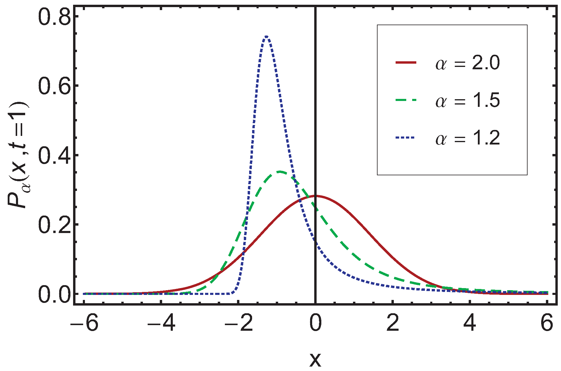
In Figure 1 a comparison plot is given, where the stable distribution $\mathbf{S}\left(\left.x\right|\alpha ,1,{\left(D_{\alpha }t\right)}^{1/\alpha },0;1\right)$ is depicted over x for $\alpha =2,1.5,1.2$. Note that $t=1$ and $D=1$ is chosen.

Figure 1. In this graph the solution $P_{\alpha }(x,t)$ for $t=1$ and $D=1$ is shown for different values of $\alpha =2.0,1.5$, and $1.2$. Note that for $\alpha =2$ the notation $P_{\mathrm{D}}(x,t)$ is used in the following.

Figure 1. In this graph the solution $P_{\alpha }(x,t)$ for $t=1$ and $D=1$ is shown for different values of $\alpha =2.0,1.5$, and $1.2$. Note that for $\alpha =2$ the notation $P_{\mathrm{D}}(x,t)$ is used in the following.

5. Kullback–Leibler Entropy

In this section we will use the Kullback–Leibler entropy as a comparison measure for the solutions of the space-fractional diffusion equation for different α. We thus aim to calculate $K(P_{\alpha },P_{\mathrm{D}})$ and $K(P_{\mathrm{D}},P_{\alpha })$.

While for standard distributions falling of fast enough as x approaches $\pm \infty$ this poses no problem, we are here concerned with distributions with heavy tails, for which we already know, that higher moments do not exist. Thus, we first have to address the question whether the Kullback–Leibler entropy exists at all. We will discuss the convergence question by using a generic Gaussian $P_{\mathrm{G}}=\mathcal{N}(\mu ,{\sigma }^2)$ and a generic $\mathbf{S}\left(\left.x\right|\alpha ,1,\gamma ,0;1\right)$ with yet unspecified γ. At the end we will replace γ by ${\gamma }_{\alpha }$.

As our aim is to establish an ordering of the distributions obtained for different α we are here interested in $K(P_{\alpha },P_{\mathrm{G}})$ as well as $K(P_{\mathrm{G}},P_{\alpha })$. We start with $K(P_{\alpha },P_{\mathrm{G}})$ and find

$$\begin{array}{cc}\hfill K(P_{\alpha },P_{\mathrm{G}})& ={\int }_{\Sigma }{P}_{\alpha }(x,t)ln\left(\frac{P_{\alpha }(x,t)}{P_{\mathrm{G}}(x,t)}\right)\mathrm{d}x\hfill \\ & ={\int }_{\Sigma }{P}_{\alpha }(x,t)ln{P}_{\alpha }(x,t)\mathrm{d}x-{\int }_{\Sigma }{P}_{\alpha }(x,t)ln{P}_{\mathrm{G}}(x,t)\mathrm{d}x\hfill \end{array}$$

(22)

The first integral of Equation (22) converges as shown in [24], whereas we will show below that the second integral does not converge and thus $K(P_{\alpha },P_{\mathrm{G}})$ does not exist. We mention here that the use of escort distributions provide an interesting route to the analysis of heavy tailed distributions in the context of the Kullback–Leibler and the q-relative entropies. For details see [48]. Their implications for the ordering of the distributions and its comparison to the bridge ordering is beyond the scope of this paper, but provides certainly an interesting starting point for further research.

For this and the following analysis we divide the integrals into three parts, the left tail, the middle part, and the right tail. Due to the known asymptotic tail behavior (18) – (20) the left tail and right tail integral can be analyzed analytically, whereas the middle part is always finite and has to be determined numerically. We split the integration domain for an arbitrary $f(x,t)$ as follows

$$\begin{array}{c}\hfill {\int }_{\Sigma }f(x,t)\mathrm{d}x={\int }_{-\infty }^{x_{-}}f(x,t)\mathrm{d}x+{\int }_{x_{-}}^{x_{+}}f(x,t)\mathrm{d}x+{\int }_{x_{+}}^{\infty }f(x,t)\mathrm{d}x\end{array}$$

(23)

where $x_{-}<0$ and $x_{+}>0$ are chosen such that for the numerical treatment the stable distributions can be well approximated by their asymptotic tail behavior. Accordingly, we have

$$\begin{array}{c}\hfill K^{†}(P_{\alpha },P_{\mathrm{G}})=K^{†}{(P_{\alpha },P_{\mathrm{G}})}_{-}+K^{†}{(P_{\alpha },P_{\mathrm{G}})}_{\pm }+K^{†}{(P_{\alpha },P_{\mathrm{G}})}_{+}\end{array}$$

(24)

We start with $K^{†}{(P_{\alpha },P_{\mathrm{G}})}_{+}$. Taking the logarithm of $P_{\mathrm{G}}(x,t)$ we find

$$ln{P}_{\mathrm{G}}(x,t)=-ln\left(\sqrt{2\pi }\sigma \right)-\frac{{(x-\mu )}^2}{2{\sigma }^2}$$

(25)

which leads to

$$\begin{array}{cc}\hfill K^{†}{(P_{\alpha },P_{\mathrm{G}})}_{+}& =ln\left(\sqrt{2\pi }\sigma \right)+{\int }_{x_{+}}^{\infty }\alpha {\gamma }^{\alpha }{c}_{\alpha }{x}^{-(\alpha +1)}\frac{{(x-\mu )}^2}{{\sigma }^2}\mathrm{d}x\hfill \end{array}$$

(26)

for the right tail integral. The range of α here is $\alpha \in (1,2)$, therefore the exponent of x of the integrand in (26) is $-\alpha +1>-1$ and thus the integral does not converge. This is compatible with the non-existence of the second moment for the stable distributions discussed here. As a result we cannot use $K(P_{\alpha },P_{\mathrm{G}})$ and thus $K(P_{\alpha },P_{\mathrm{D}})$ as a basis for defining a distance measure on the distributions in the transition regime between reversible and irreversible processes.

As the Kullback–Leibler entropy is an asymmetric measure, the non-existence of $K(P_{\alpha },P_{\mathrm{G}})$ does not imply the non-existence of $K(P_{\mathrm{G}},P_{\alpha })$ which we now analyze

$$\begin{array}{cc}\hfill K(P_{\mathrm{G}},P_{\alpha })& ={\int }_{\Sigma }{P}_{\mathrm{G}}(x,t)ln\left(\frac{P_{\mathrm{G}}(x,t)}{P_{\alpha }(x,t)}\right)\mathrm{d}x\hfill \\ & ={\int }_{\Sigma }{P}_{\mathrm{G}}(x,t)ln{P}_{\mathrm{G}}(x,t)\mathrm{d}x-{\int }_{\Sigma }{P}_{\mathrm{G}}(x,t)ln{P}_{\alpha }(x,t)\mathrm{d}x\hfill \end{array}$$

(27)

The first integral yields

$$\begin{array}{cc}\hfill {\int }_{\Sigma }{P}_{\mathrm{G}}(x,t)ln{P}_{\mathrm{G}}(x,t)\mathrm{d}x& =-1/2(1+ln\left(2\pi {\sigma }^2\right))\hfill \end{array}$$

(28)

which is finite.

For the further discussion below we recall that

$$\begin{array}{c}\hfill {\int }_{x_{+}}^{\infty }{x}^a{e}^{-c{x}^d}\mathrm{d}x<\infty \mathrm{and}{\int }_{x_{+}}^{\infty }ln\left(x\right)e^{-c{x}^d}\mathrm{d}x<\infty \end{array}$$

(29)

for any given $c>0$, $d>0$, and a arbitrary but fixed. The logarithm $ln{P}_{\alpha }(x,t)$ within the second integral of (27) is obtained from the asymptotic tail behavior. For the right tail we get

$$\begin{array}{cc}\hfill ln\left(P_{\alpha }(x\to +\infty ,t)\right)& =ln\left(2\alpha c_{\alpha }\right)+ln{\gamma }^{\alpha }-(\alpha +1)lnx\hfill \end{array}$$

(30)

which according to (29) converges. For the left tail we have

$$\begin{array}{cc}\hfill ln\left(P_{\alpha }(x\to -\infty ,t)\right)& =ln{C}_1+\frac{2-\alpha }{2\alpha -2}ln\left(-\frac{x}{\gamma }\right)-C_2{\left(-\frac{x}{\gamma }\right)}^{\frac{\alpha }{\alpha -1}}\hfill \end{array}$$

(31)

Multiplied with $P_{\mathrm{G}}$, one finds from (29) that the integrals converge for $\alpha \in (1,2)$.

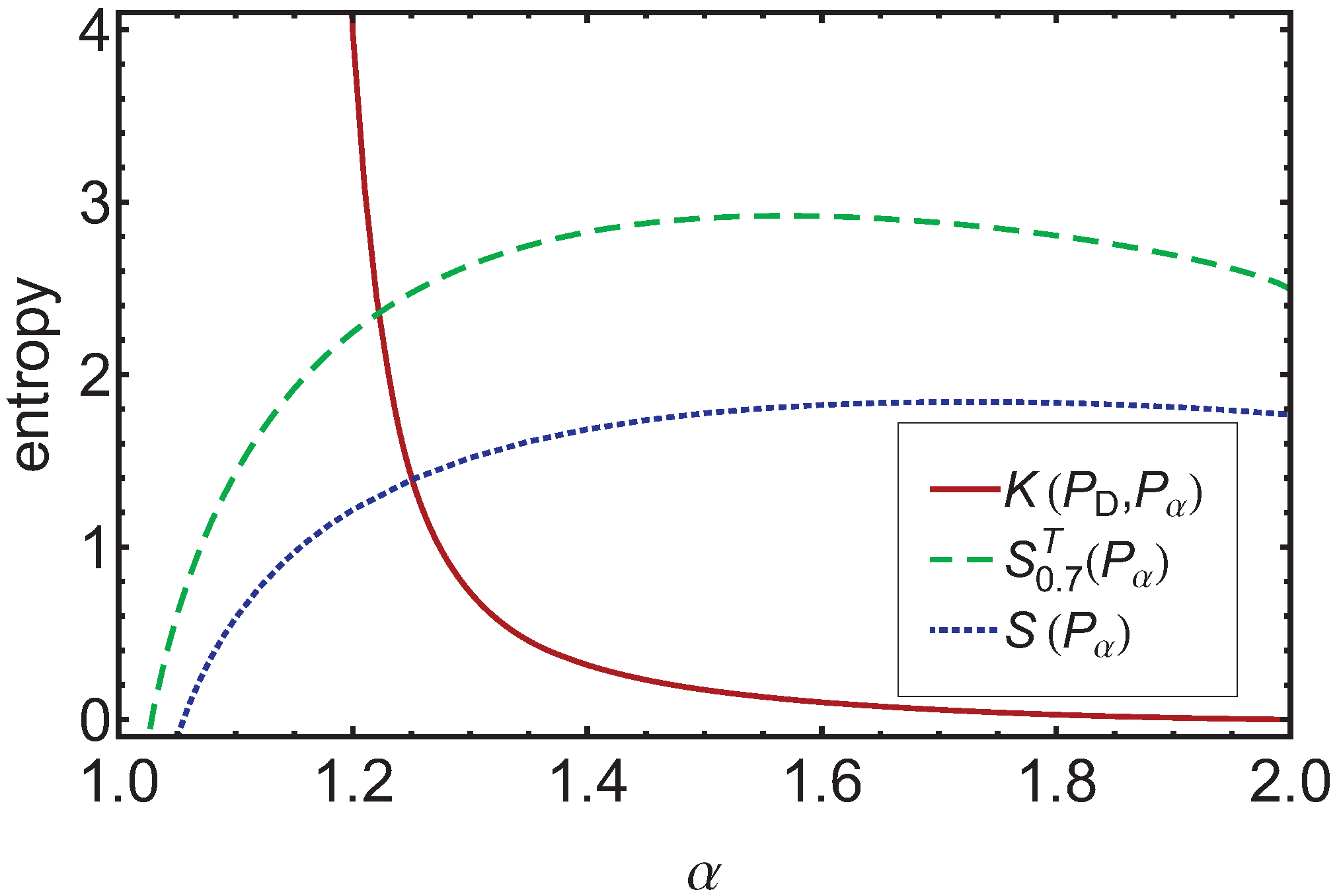
As a result $K(P_{\mathrm{G}},P_{\alpha })$ and thus $K(P_{\mathrm{D}},P_{\alpha })$ can provide a new basis of comparison between the probability distributions for different α. In Figure 2 we show $K(P_{\mathrm{D}},P_{\alpha })$ as a function of α for time $t=1$. The monotonous dependence indicates that $K(P_{\mathrm{D}},P_{\alpha })$ provides the same ordering of the diffusion processes in the bridging regime as does the entropy production rate, albeit in reversed order. The $K(P_{\mathrm{D}},P_{\alpha })$-ordering is fully compatible with the ordering obtained by using the Shannon entropy and the Tsallis entropy as a means of comparison, when the appropriate times are chosen for the different processes, such that the internal quickness is separated out [24]. If one does not separate out the internal quickness, then the Shannon entropy $S\left(P_{\alpha }\right)$ as well as the Tsallis entropy $S_q^{\mathrm{T}}\left(P_{\alpha }\right)$, see [24], provides an ordering not compatible with the bridge ordering. The corresponding curves for $t=1$ are shown in Figure 2, too.

Figure 2. Here the Kullback–Leibler entropy $K(P_{\mathrm{D}},P_{\alpha })$, the Tsallis entropy $S_{q=0.7}^{\mathrm{T}}\left(P_{\alpha }\right)$ and the Shannon entropy $S\left(P_{\alpha }\right)$ are plotted over α at $t=1$. We can see that the Kullback–Leibler entropy shows a monotonic decreasing behavior for increasing α, whereas the Tsallis and the Shannon entropy exhibit a maximum. Thus, $K(P_{\mathrm{D}},P_{\alpha })$ is an appropriate ordering measure for the bridging regime even when other measure candidates are not monotonic.

Figure 2. Here the Kullback–Leibler entropy $K(P_{\mathrm{D}},P_{\alpha })$, the Tsallis entropy $S_{q=0.7}^{\mathrm{T}}\left(P_{\alpha }\right)$ and the Shannon entropy $S\left(P_{\alpha }\right)$ are plotted over α at $t=1$. We can see that the Kullback–Leibler entropy shows a monotonic decreasing behavior for increasing α, whereas the Tsallis and the Shannon entropy exhibit a maximum. Thus, $K(P_{\mathrm{D}},P_{\alpha })$ is an appropriate ordering measure for the bridging regime even when other measure candidates are not monotonic.

6. Tsallis Relative Entropy

Now, we turn to the Tsallis relative entropy. In the following section we will analyze for which values of the non-extensivity parameter q the integrals do converge. For this analysis we assume again a generic Gaussian and a generic stable distribution. Afterwards, we present the numerical results.

We start with $T_q(P_{\alpha },P_{\mathrm{G}})$, for which we have

$$\begin{array}{cc}\hfill T_q(P_{\alpha },P_{\mathrm{G}})& =\frac{1}{q-1}\left({\int }_{\Sigma }\frac{P_{\alpha }^q(x,t)}{P_{\mathrm{G}}^{q-1}(x,t)}\mathrm{d}x-1\right)\hfill \\ & =\frac{1}{q-1}\left({\int }_{\Sigma }{\left(\sqrt{2\pi }\sigma \right)}^{q-1}\frac{\mathbf{S}{\left(\left.x\right|\alpha ,1,\gamma ,0;1\right)}^q}{exp{\left(-\frac{{(x-\mu )}^2}{2{\sigma }^2}\right)}^{q-1}}\mathrm{d}x-1\right)\hfill \\ & =\frac{1}{q-1}\left(\frac{{\left(\sqrt{2\pi }\sigma \right)}^{q-1}}{{\gamma }^q}{\int }_{\Sigma }\frac{\mathbf{S}{\left(\left.\frac{x}{\gamma }\right|\alpha ,1,1,0;1\right)}^q}{exp{\left(-\frac{{(x-\mu )}^2}{2{\sigma }^2}\right)}^{q-1}}\mathrm{d}x-1\right)\hfill \end{array}$$

(32)

In analogy to the analysis of the Kullback–Leibler entropy, (23) and (24) , we split the Tsallis relative entropy integral into three parts, left tail, middle part, and right tail. Due to the asymptotic tail behavior of the stable distribution given in (18) and (20) we can investigate the left and the right tail analytically. For the Tsallis relative entropy we thus have

$$\begin{array}{cc}\hfill T_q(P_{\alpha },P_{\mathrm{G}})& =\frac{1}{q-1}\left((T_q{(P_{\alpha },P_{\mathrm{G}})}_{-}+T_q{(P_{\alpha },P_{\mathrm{G}})}_{\pm }+T_q{(P_{\alpha },P_{\mathrm{G}})}_{+})-1\right)\hfill \end{array}$$

(33)

The left tail integral yields

$$\begin{array}{c}{T}_q{(P_{\alpha },P_{\mathrm{G}})}_{-}\hfill \end{array}$$

$$\begin{array}{cc}& =\frac{{\left(\sqrt{2\pi }\sigma \right)}^{q-1}}{{\gamma }^q}{\int }_{-\infty }^{x_{-}}{\left(C_1{\left(-\frac{x}{\gamma }\right)}^{\frac{2-\alpha }{2\alpha -2}}exp\left(-C_2{\left(-\frac{x}{\gamma }\right)}^{\frac{\alpha }{\alpha -1}}\right)\right)}^{q}exp{\left(-\frac{{(x-\mu )}^2}{2{\sigma }^2}\right)}^{1-q}\mathrm{d}x\hfill \\ & =\frac{{\left(\sqrt{2\pi }\sigma \right)}^{q-1}}{{\gamma }^q}{\int }_{-\infty }^{x_{-}}{C}_1^q{\left(-\frac{x}{\gamma }\right)}^{\frac{q(2-\alpha )}{2\alpha -2}}exp\left(-q{C}_2{\left(-\frac{x}{\gamma }\right)}^{\frac{\alpha }{\alpha -1}}-(1-q)\frac{{(x-\mu )}^2}{2{\sigma }^2}\right)\mathrm{d}x\hfill \end{array}$$

(34)

First, we note that the constant $C_2$ takes values from 0 to $\frac{1}{4}$ monotonically increasing for $\alpha \in (1,2)$. Also we find that the exponent $\alpha /(\alpha -1)$ lies within the range of $(\infty ,2)$ for $\alpha \in (1,2)$. Thus, the first term in the exponent of the exponential will dominate the second one and the integral will converge if the prefactor $-q{C}_2$ of that term is negative, whereas for $q=1$ the second term takes over. This sets $q\ge 0$ as a first requirement.

For the right tail integral $T_q{(P_{\alpha },P_{\mathrm{G}})}_{+}$ we obtain

$$\begin{array}{cc}\hfill T_q{(P_{\alpha },P_{\mathrm{G}})}_{+}& ={\int }_{x_{+}}^{\infty }{\left(2\alpha \gamma c_{\alpha }{x}^{-(\alpha +1)}\right)}^q{\left(\sqrt{2\pi }\sigma \right)}^{q-1}exp{\left(-\frac{{(x-\mu )}^2}{2{\sigma }^2}\right)}^{1-q}\mathrm{d}x\hfill \\ & ={\int }_{x_{+}}^{\infty }{\left(2\alpha \gamma c_{\alpha }\right)}^q{\left(\sqrt{2\pi }\sigma \right)}^{q-1}{x}^{-q(\alpha +1)}exp\left(-(1-q)\frac{{(x-\mu )}^2}{2{\sigma }^2}\right)\mathrm{d}x\hfill \end{array}$$

(35)

that converges for $1-q>0$ or $q<1$. This sets the second requirement on q. Overall, the Tsallis relative entropy $T_q(P_{\alpha },P_{\mathrm{G}})$ and thus $T_q(P_{\alpha },P_{\mathrm{D}})$ exist for $q\in [0,1)$.

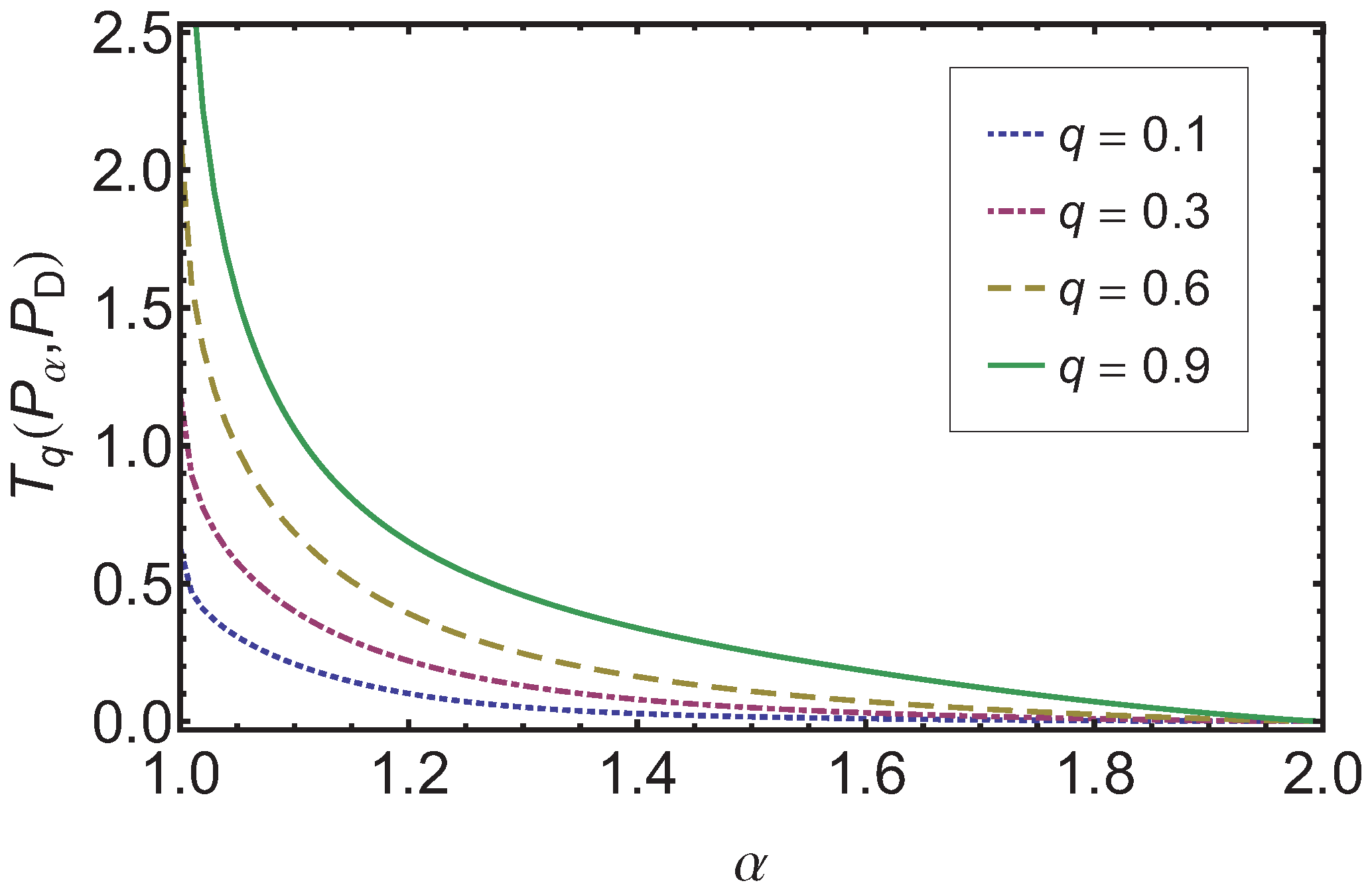
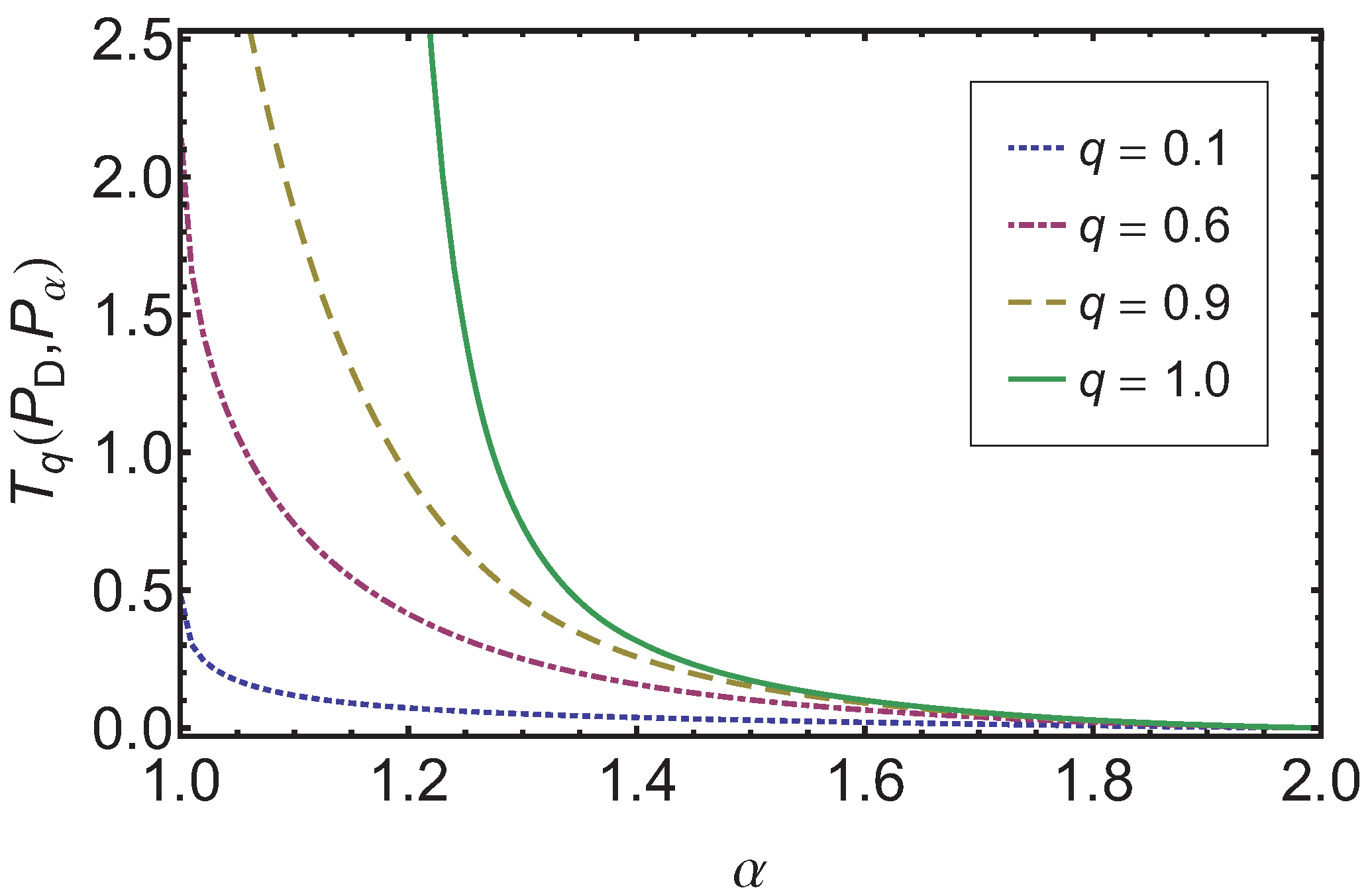
In Figure 3 the dependence of $T_q(P_{\alpha },P_{\mathrm{D}})$ on α is shown. Again one finds an ordering compatible with the original order as established by α, the bridge ordering. This holds independent of the q value used as long as $q\in [0,1)$. We note that the larger q is the easier it is to separate two processes with different α. Also as expected for $\alpha \to 2$ the measure goes to zero, independent of $q\in [0,1)$.

Figure 3. The results for the Tsallis relative entropy $T_q(P_{\alpha },P_{\mathrm{D}})$ are shown over α for four different values of q ($q=0.1,0.3,0.6$, and $0.9$). As expected $T_q(P_{\alpha },P_{\mathrm{D}})$ goes to zero as α approaches 2, independent of q.

Figure 3. The results for the Tsallis relative entropy $T_q(P_{\alpha },P_{\mathrm{D}})$ are shown over α for four different values of q ($q=0.1,0.3,0.6$, and $0.9$). As expected $T_q(P_{\alpha },P_{\mathrm{D}})$ goes to zero as α approaches 2, independent of q.

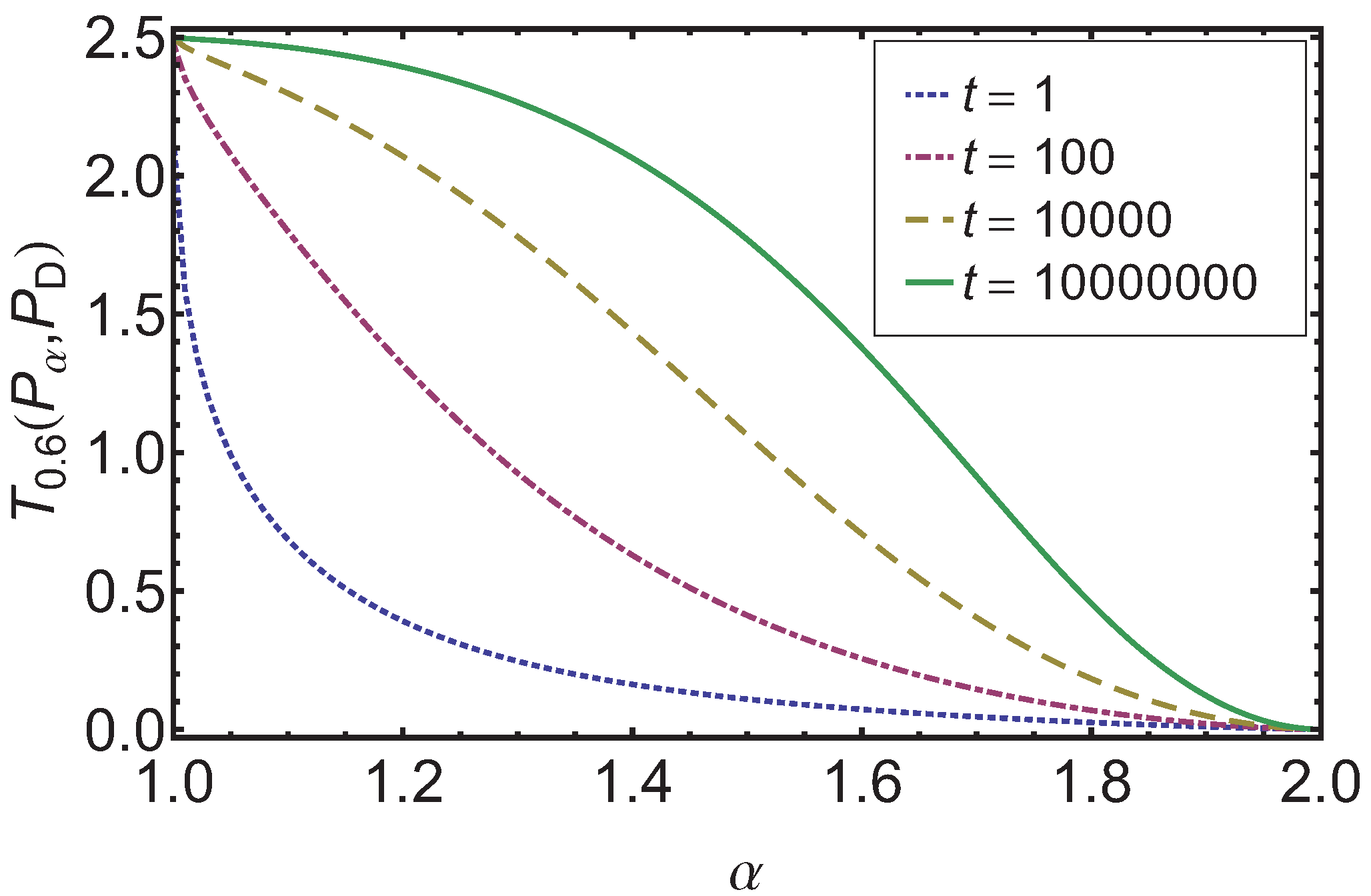
While the complete discussion of the time development of the Tsallis relative entropy is beyond the scope of this paper, we show in Figure 4 how $T_q(P_{\alpha },P_{\mathrm{D}})$ (for $q=0.6$) behaves for different times. One sees that the monotonic behavior is preserved. An interesting question for future research is whether one can formulate an extension of the H-theorem for this measure.

Figure 4. For the case of $q=0.6$ the results for the Tsallis relative entropy $T_{0.6}(P_{\alpha },P_{\mathrm{D}})$ for different times t is given over α. One can observe that with increasing time the monotonic decreasing behavior is preserved.

Figure 4. For the case of $q=0.6$ the results for the Tsallis relative entropy $T_{0.6}(P_{\alpha },P_{\mathrm{D}})$ for different times t is given over α. One can observe that with increasing time the monotonic decreasing behavior is preserved.

Finally, we analyze for which values of q the Tsallis relative entropy $T_q(P_{\mathrm{G}},P_{\alpha })$ does exist. It is given as

$$\begin{array}{cc}\hfill T_q(P_{\mathrm{G}},P_{\alpha })& =\frac{1}{q-1}\left({\int }_{\Sigma }{\left(\frac{1}{\sqrt{2\pi }\sigma }\right)}^q\frac{exp{\left(-\frac{{(x-\mu )}^2}{2{\sigma }^2}\right)}^q}{\mathbf{S}{\left(\left.x\right|\alpha ,1,\gamma ,0;1\right)}^{q-1}}\mathrm{d}x-1\right)\hfill \\ & =\frac{1}{q-1}\left({\int }_{\Sigma }\frac{{\gamma }^{(q-1)}}{{\left(\sqrt{2\pi }\sigma \right)}^q}\frac{exp{\left(-\frac{{(x-\mu )}^2}{2{\sigma }^2}\right)}^q}{\mathbf{S}{\left(\left.\frac{x}{\gamma }\right|\alpha ,1,1,0;1\right)}^{q-1}}\mathrm{d}x-1\right)\hfill \end{array}$$

(36)

Again we have to investigate the tail integrals based on the asymptotic tail behaviors that are given in (20) and (18) . We split our integral into three part as explained in (33) and in the case of the (36) we obtain the subsequent left tail integral $T_q{(P_{\mathrm{G}},P_{\alpha })}_{-}$ as

$$\begin{array}{cc}& T_q{(P_{\mathrm{G}},P_{\alpha })}_{-}\hfill \end{array}$$

$$\begin{array}{cc}& =\frac{{\gamma }^{(q-1)}}{{\left(\sqrt{2\pi }\sigma \right)}^q}{\int }_{-\infty }^{x_{-}}exp{\left(-\frac{{(x-\mu )}^2}{2{\sigma }^2}\right)}^q{\left(C_1{\left(\frac{-x}{\gamma }\right)}^{\frac{2-\alpha }{2\alpha -2}}exp\left(-C_2{\left(\frac{-x}{\gamma }\right)}^{\frac{\alpha }{\alpha -1}}\right)\right)}^{1-q}\mathrm{d}x\hfill \\ & =\frac{{\gamma }^{(q-1)}}{{\left(\sqrt{2\pi }\sigma \right)}^q}{\int }_{-\infty }^{x_{-}}{C}_1^{1-q}{\left(\frac{-x}{\gamma }\right)}^{\frac{(1-q)(2-\alpha )}{2\alpha -2}}exp\left(-q\frac{{(x-\mu )}^2}{2{\sigma }^2}-(1-q)C_2{\left(\frac{-x}{\gamma }\right)}^{\frac{\alpha }{\alpha -1}}\right)\mathrm{d}x\hfill \end{array}$$

(37)

In order to find the requirement on q we proceed in analogy to the discussion for (34) . Here the second term of the exponent of the exponential in the integrand will dominate the first term for large enough $\left|x\right|$. Thus the prefactor must not be negative for convergence, i.e., $(1-q)C_2>0$, or it is zero and then the first term takes over, and thus the requirement is $q<1$, as for $q=1$ the Tsallis relative entropy is not defined.

For the right tail integral $T_q{(P_{\mathrm{G}},P_{\alpha })}_{+}$ we get

$$\begin{array}{cc}\hfill T_q{(P_{\mathrm{G}},P_{\alpha })}_{+}& ={\int }_{x_{+}}^{\infty }{\left(\frac{1}{\sqrt{2\pi }\sigma }exp\left(-\frac{{(x-\mu )}^2}{2{\sigma }^2}\right)\right)}^q{\left(2\alpha {\gamma }^{\alpha }{c}_{\alpha }{x}^{-(\alpha +1)}\right)}^{1-q}\mathrm{d}x\hfill \\ & ={\int }_{x_{+}}^{\infty }{\left(\frac{1}{\sqrt{2\pi }\sigma }\right)}^q{\left(2\alpha {\gamma }^{\alpha }{c}_{\alpha }\right)}^{1-q}{x}^{-(1-q)(\alpha +1)}exp\left(-q\frac{{(x-\mu )}^2}{2{\sigma }^2}\right)\mathrm{d}x\hfill \end{array}$$

(38)

which converges for all $\alpha \in (1,2)$ for $q\ge 0$. Therefore, q has to be in the range $[0,1)$ in order to insure that the Tsallis relative entropy $T_q(P_{\mathrm{G}},P_{\alpha })$ has a finite value.

In Figure 5 we show the dependence of $T_q(P_{\mathrm{D}},P_{\alpha })$ on α. The ordering of the superdiffusion processes in the bridging regime induced by $T_q(P_{\mathrm{D}},P_{\alpha })$ is again in full agreement with the bridge ordering by α.

Figure 5. Here, the Tsallis relative entropy $T_q(P_{\mathrm{D}},P_{\alpha })$ is depicted over α for different values of q. We find that for $\alpha \to 2$$T_q(P_{\mathrm{D}},P_{\alpha })$ goes down to zero, independent of q. Note that in the case of $q=1$ the corresponding Kullback–Leibler entropy is shown.

Figure 5. Here, the Tsallis relative entropy $T_q(P_{\mathrm{D}},P_{\alpha })$ is depicted over α for different values of q. We find that for $\alpha \to 2$$T_q(P_{\mathrm{D}},P_{\alpha })$ goes down to zero, independent of q. Note that in the case of $q=1$ the corresponding Kullback–Leibler entropy is shown.

As both relative entropies, the Kullback–Leibler $K(P_{\mathrm{D}},P_{\alpha })$ as well as the Tsallis relative entropy $T_q(P_{\mathrm{D}},P_{\alpha })$, preserve the ordering of the processes in the superdiffusion regime as induced by α, it is interesting to study their relative behavior. In Figure 6 a log-log-plot of $K(P_{\mathrm{D}},P_{\alpha })$ versus $T_q(P_{\mathrm{D}},P_{\alpha })$ is shown for different q and identical $P_{\alpha }$ and $P_{\mathrm{D}}$. The graph shows a clear monotonic relationship independent of the q value used. As $T_q(P_{\mathrm{D}},P_{\alpha })$ approaches $K(P_{\mathrm{D}},P_{\alpha })$ in the limit $q\to 1$ the close to straight line for $q=0.95$ is expected. Interestingly, the curves for the other q values also show this feature for small values of the relative entropies.

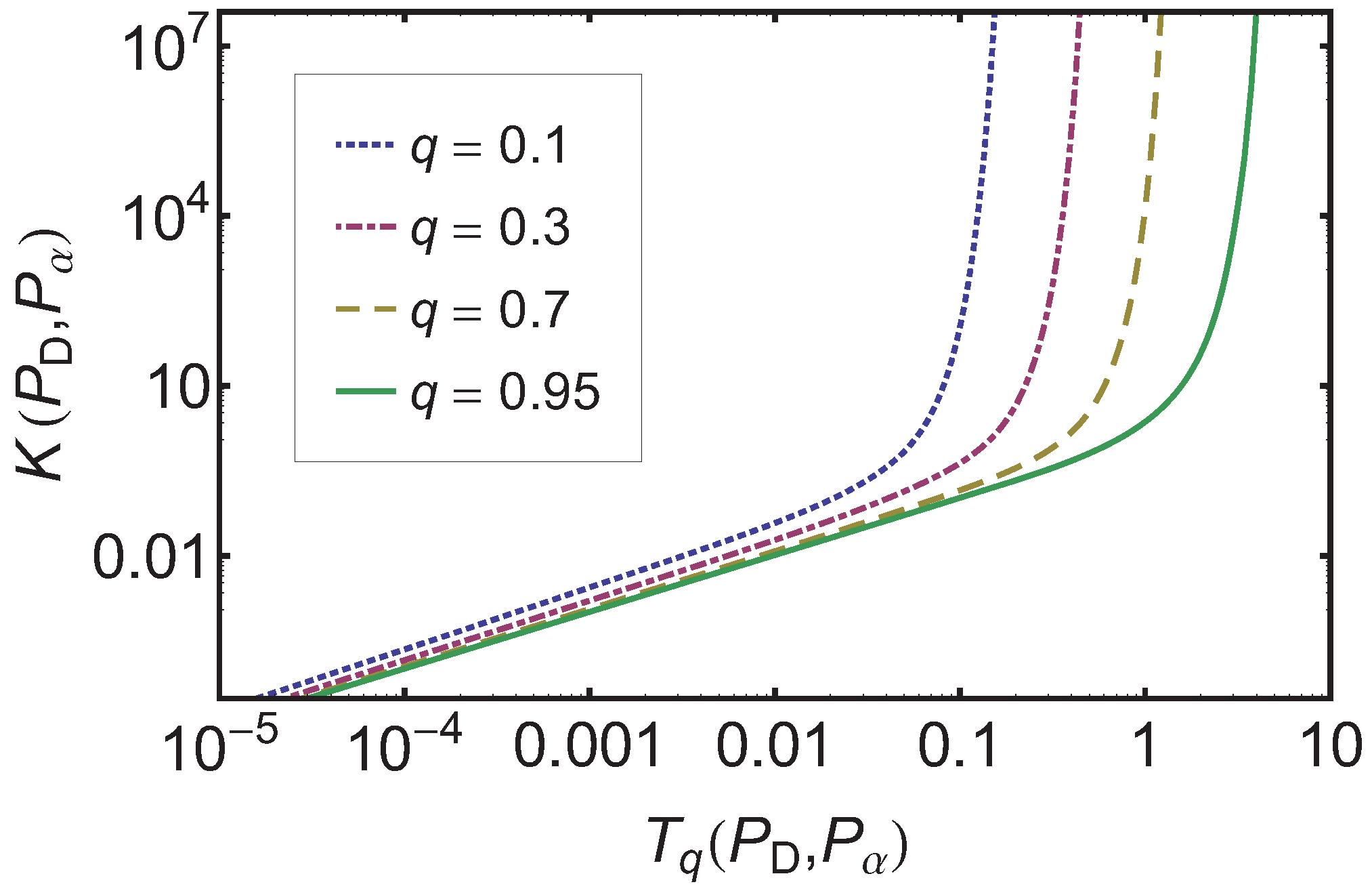
Figure 6. The log-log-plot of the Kullback–Leibler entropy $K(P_{\mathrm{D}},P_{\alpha })$ over the Tsallis relative entropy $T_q(P_{\mathrm{D}},P_{\alpha })$ for different q-values is given. A clear monotonic monotonic relationship is observed independent of q.

Figure 6. The log-log-plot of the Kullback–Leibler entropy $K(P_{\mathrm{D}},P_{\alpha })$ over the Tsallis relative entropy $T_q(P_{\mathrm{D}},P_{\alpha })$ for different q-values is given. A clear monotonic monotonic relationship is observed independent of q.

7. Summary and Discussion

The bridge ordering by α of the space-fractional diffusion equations and of the corresponding PDFs $P_{\alpha }(x,t)$ had previously shown a structure not compatible with an ordering based on the Shannon, the Tsallis, and the Rényi entropies, and their respective rates. While we were able to resolve this behavior known as the entropy production paradox by an in depth analysis of the intricate coupling of internal quickness to the form change of the PDFs, we here found that the Kullback or Kullback–Leibler entropy and its generalization, the Tsallis relative entropy, naturally establish an ordering on the $P_{\alpha }(x,t)$ consistent with the bridge ordering. We did this by calculating the Kullback entropy and the Tsallis relative entropy with respect to the solution of the regular diffusion equation, i.e., the $\alpha =2$ case of the space-fractional diffusion equation.

We found that the Kullback–Leibler entropy for a $P_{\alpha }$ versus a general Gaussian distribution does not exist as the integrals diverge. The reason for this divergence is rooted in the heavy tails of the stable distributions. These heavy tails lead to the non-existence of higher moments, and considering the fact that the logarithm of a Gaussian is proportional to the second moment, the divergence of the Kullback–Leibler entropy is not surprising.

The Tsallis relative entropy, which is a non-extensive extension of the Kullback–Leibler entropy depending on a non-extensivity parameter $q\in \mathbb{R}/\left\{1\right\}$, however does exist and thus proves to be a highly useful generalization of the Kullback–Leibler entropy. In particular we showed that the Tsallis relative entropy can be determined for q-values in the range $q\in [0,1)$. Within that range the Tsallis relative entropy of $P_{\alpha }$ with respect to $P_{\mathrm{D}}$ as well as Tsallis relative entropy of $P_{\mathrm{D}}$ with respect to $P_{\alpha }$ for all q show an ordering of the $P_{\alpha }$ consistent with the bridge ordering as induced by α.