Thermodynamic Modeling for Open Combined Regenerative Brayton and Inverse Brayton Cycles with Regeneration before the Inverse Cycle

Abstract

A thermodynamic model of an open combined regenerative Brayton and inverse Brayton cycles with regeneration before the inverse cycle is established in this paper by using thermodynamic optimization theory. The flow processes of the working fluid with the pressure drops and the size constraint of the real power plant are modeled. There are 13 flow resistances encountered by the working fluid stream for the cycle model. Four of these, the friction through the blades and vanes of the compressors and the turbines, are related to the isentropic efficiencies. The remaining nine flow resistances are always present because of the changes in flow cross-section at the compressor inlet of the top cycle, regenerator inlet and outlet, combustion chamber inlet and outlet, turbine outlet of the top cycle, turbine outlet of the bottom cycle, heat exchanger inlet, and compressor inlet of the bottom cycle. These resistances associated with the flow through various cross-sectional areas are derived as functions of the compressor inlet relative pressure drop of the top cycle, and control the air flow rate, the net power output and the thermal efficiency. The analytical formulae about the power output, efficiency and other coefficients are derived with 13 pressure drop losses. It is found that the combined cycle with regenerator can reach higher thermal efficiency but smaller power output than those of the base combined cycle at small compressor inlet relative pressure drop of the top cycle.

1. Introduction

Thermodynamic optimization theory [1,2,3,4,5,6,7,8,9,10,11,12,13,14,15,16,17,18,19,20,21,22,23,24] is a powerful tool for the performance analysis and optimization of various thermodynamic processes and cycles. In the current studies, performance analysis for Brayton (gas turbine) cycles has made tremendous progress by using thermodynamic optimization theory. For the open Brayton cycles, which are widely used in industry practice, the principle of optimally tuning the air flow rate and subsequent distribution of pressure drops has been used [25,26,27,28,29,30,31]. The analogy between the irreversibility of heat transfer across a finite temperature difference (thermal resistance) and the irreversibility of fluid flow across a finite pressure drop (fluid flow resistance) was exploited by Bejan [25] and Radcenco [26], and was further studied by Bejan [27,28], Chen et al. [29,30] and Hu and Chen [31]. It had been proved that there existed an optimal pressure drop for fluid flow process.

A thermodynamic model of an open simple Brayton cycle with pressure drop irreversibility was established by Radcenco et al. [32]. They derived the function relations about the compressor power input, the heat released rate produced by the burning fuel, the turbine power output, the rate of heat released by the exhaust, the cycle power output, the cycle thermal efficiency and the pressure loss of the components due to the flow irreversibility of the working fluid versus the compressor inlet relative pressure drop. They also provided numerical results for the analysis and optimization of the cycle power output, and the analysis and optimization results of the cycle thermal efficiency under the constrains of the fuel consumption and the overall flow area, respectively. Chen et al. [33] optimized the power and efficiency of an open-cycle regenerative Brayton cycle by using a similar method. It was found that the regenerative Brayton cycle can attain higher thermal efficiency than that of the simple Brayton cycle but with smaller power output. Wang et al. [34] optimized the power and the efficiency of an open-cycle intercooled Brayton cycle. The numerical examples showed that the increase in the effectiveness of intercooler increases both the maximum cycle thermodynamic first-law efficiency and the maximum net power output. Zhang et al. [35,36] optimized the performance of an open-cycle gas turbine power plant with a refrigeration cycle for compressor inlet air cooling. It was found that the net power output and thermal efficiency are improved by using the refrigeration cycle for compressor air inlet cooling. Chen et al. [37] optimized the performance of a thermodynamic model for an open regenerative cycle of an externally fired micro gas turbine power plant.

In order to meet the increased request to the effective thermodynamic cycles, more and more new cycle models have been proposed in recently years. Agnew et al. [38] proposed combined Brayton and inverse Brayton cycles in 2003, and performed the first law analysis of the combined cycle by using the commercial process simulation package. It revealed that this combined cycle’s performance is superior to the simple gas turbine cycle and suitable for low-grade cogeneration applications. The exergy analysis and optimization of the combined Brayton and inverse Brayton cycles were performed by Zhang et al. [39]. Based on the combined Brayton and inverse Brayton cycles, Alabdoadaim et al. [40,41,42] proposed its developed configurations including regenerative cycle and reheat cycle, and using two parallel inverse Brayton cycles as bottom cycles. They found that the system with regeneration attains higher heat efficiency than that of the base system, but with smaller work output based on the first law analysis. Zhang et al. [43] performed exergy analysis of the combined Brayton and two parallel inverse Brayton cycles.

Analysis of thermodynamic cycles based on the first law and the second law are usually used when proposing new cycle configurations such as the combined Brayton and (two parallel) inverse Brayton cycles. In order to know more about the performance of the new configurations, Zhang et al. [44] studied the performance of the combined Brayton and inverse Brayton cycles by using the thermodynamic optimization theory. The power and the thermal efficiency were optimized by adjusting the bottom cycle pressure ratio and the mass flow rate. Moreover, they studied the performance of the combined Brayton and two parallel inverse Brayton cycles [45,46]. A further step of this paper beyond [37,42,44,45,46] is to analyze and optimize the performance of the combined regenerative Brayton and inverse Brayton cycles proposed in [42] with consideration of the pressure drops and the size constraints by using similar principles and methods as used in [25,26,27,28,29,30,31].

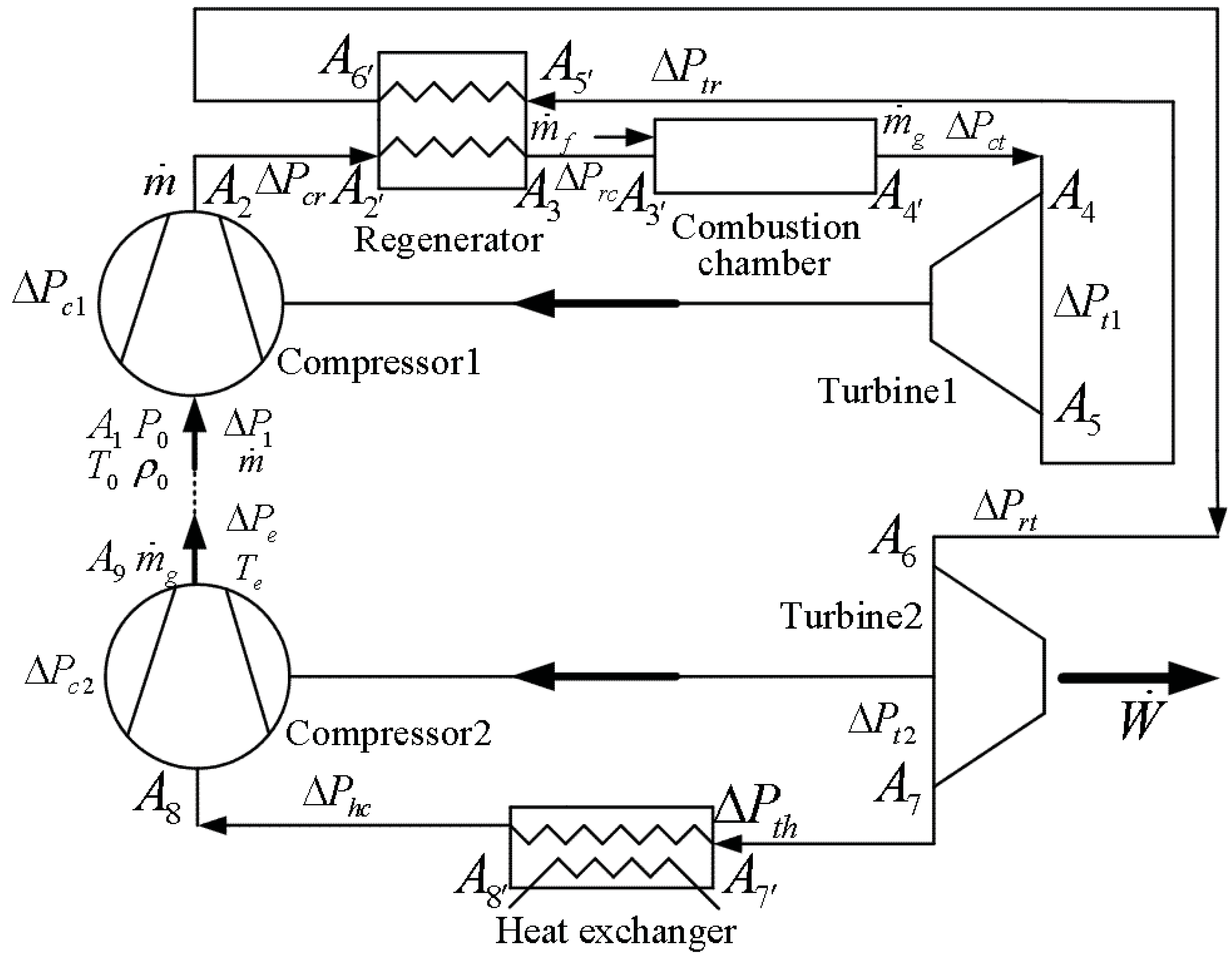
2. Physical Model

The system proposed in [42] is shown in Figure 1. It is constructed from a top cycle (regenerative Brayton cycle) and a bottom cycle (inverse Brayton cycle). The top cycle is used as a gas generator to power the bottom cycles. The purpose of the turbine in the top cycle is solely to power the compressor of the top cycle. The power output of the combined cycle is totally produced by the bottom cycle. This combined regenerative Brayton and inverse Brayton cycles recover heat energy before the working fluid entering the turbine of the inverse Brayton cycle.

Figure 1. Pressure drop and mass flow rate distributions for the combined regenerative Brayton and inverse Brayton cycles.

Figure 1. Pressure drop and mass flow rate distributions for the combined regenerative Brayton and inverse Brayton cycles.

Proceeding along the path followed by the working fluid, the following modeling assumptions are made:

(1)

The working fluid (air, gas) is an ideal gas with a specific heat that depends on temperature and composition.

(2)

The air flows into the compressor of the top cycle (process 0 − 1) irreversibly and accompanied by the pressure drop $\Delta P_1=P_0-P_1$ and the entropy increase $\Delta s_1$ at the ambient temperature $T_0$ [26]. In the following analysis, $P$ represents overall pressure.

(3)

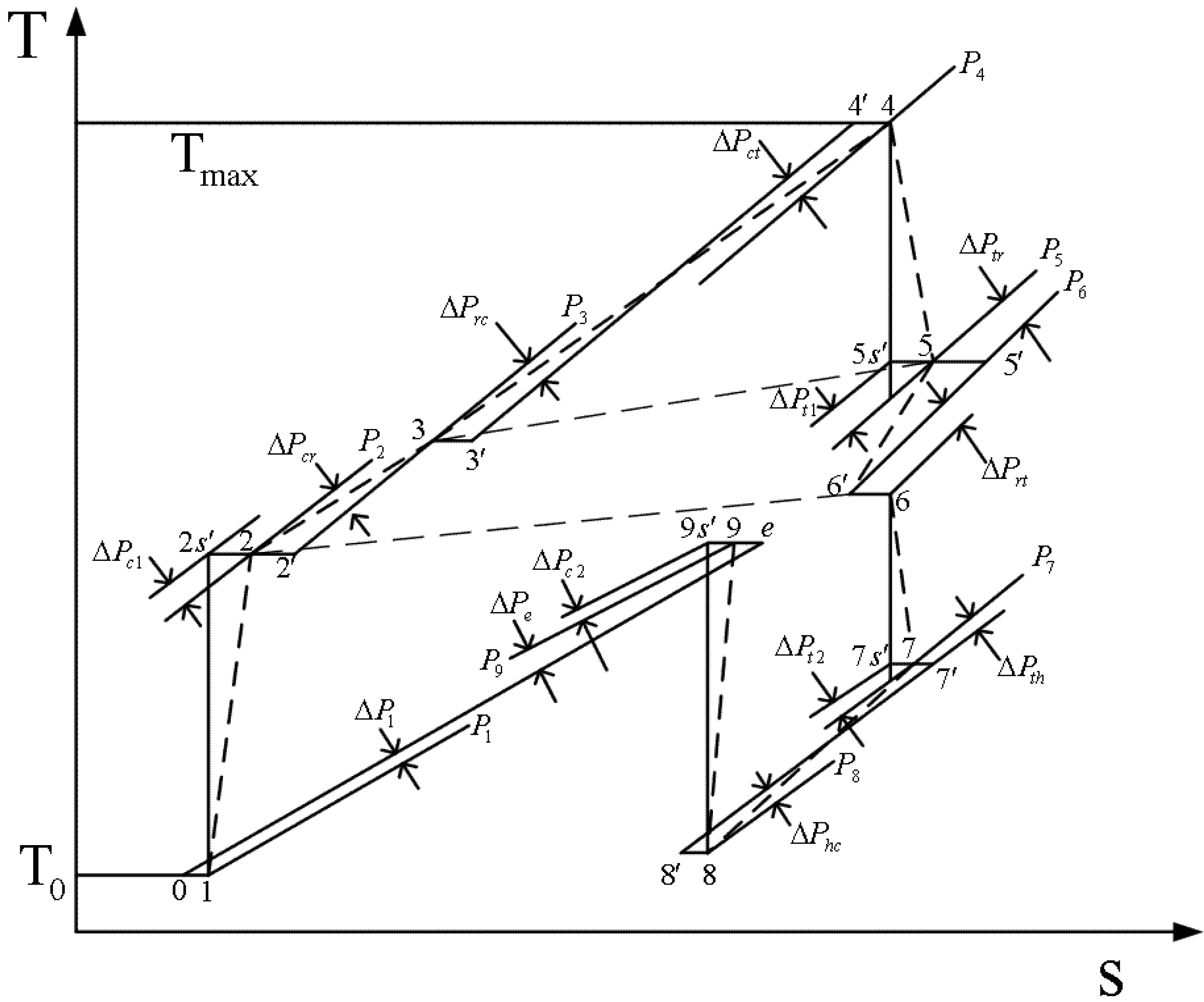
The air compression process 1 − 2 of the top cycle is adiabatic and irreversible, leading to the entropy increase $\Delta s_{c1}$. In Figure 2 this process is represented schematically by the isentropic compression $1-2s^{\prime }$ followed by the throttling process $2s^{\prime }-2$, which accounts for the pressure drop $\Delta P_{c1}$ associated with fluid friction through the compressor stages of the top cycle.

(4)

The air flows into the cold-side of the regenerator (process 2 − 3) irreversibly and accompanied by the pressure drop $\Delta P_{cr}$. In Figure 2 this process is represented schematically by the throttling process $2-2^{\prime }$ (entropy increase is $\Delta s_{cr}$) followed by the isobaric absorbed heat process $2^{\prime }-3$ (pressure is $P^{\prime }=P_3=P_2-\Delta P_{cr}$).

(5)

The combustion process (process $3-4^{\prime }$) and flow through the combustion chamber are characterized by the pressure drop $\Delta P_{rc}$. In Figure 2 this process is represented schematically by the throttling process $3-3^{\prime }$ (entropy increase $\Delta s_{rc}$) followed by the isobaric absorbed heat process $3^{\prime }-4^{\prime }$ (pressure is $P^{″}=P_{4^{\prime }}=P_3-\Delta P_{rc}$). A fraction (${\dot{Q}}_{cf}$) of the heating rate produced by the burning fuel (${\dot{Q}}_f$) leaks directly into the ambient through the walls of the combustion chamber [25,26,28].

(6)

The pressure drop associated with the flow out of the combustion chamber and into the turbine 1 (process $4^{\prime }-4$) is $\Delta P_{ct}$. The process is a accompanied by the entropy increase $\Delta s_{ct}$.

(7)

The turbine 1 expansion process 4 − 5 of the top cycle is modeled as adiabatic and irreversible with the entropy increase $\Delta s_{t1}$. In Figure 2 this process is represented schematically by the isentropic expansion $4-5s^{\prime }$ from $P_4=P_{4^{\prime }}-\Delta P_{ct}$ to $P_{5s^{\prime }}=P_5+\Delta P_{t1}$, followed by the adiabatic throttling process $5s^{\prime }-5$ accounting for the pressure drop $\Delta P_{t1}$ through the blades and vanes of the turbine of the top cycle.

(8)

The air flows into the hot-side of the regenerator (process $5-6^{\prime }$) irreversibly and accompanied by the pressure drop $\Delta P_{tr}$. In Figure 2 this process is represented schematically by the throttling process $5-5^{\prime }$ (entropy increase is $\Delta s_{tr}$) followed by the isobaric evolved heat process $5^{\prime }-6^{\prime }$ (pressure is $P_{6^{\prime }}=P_5-\Delta P_{tr}$).

(9)

The pressure drop associated with the flow out of the hot-side of the regenerator and into the turbine 2 (process $6^{\prime }-6$) is $\Delta P_{rt}$. The process is a accompanied by the entropy increase $\Delta s_{rt}$.

(10)

The turbine expansion process $6-7$ of the top cycle is modeled as adiabatic and irreversible with the entropy increase $\Delta s_{t2}$. In Figure 2 this process is equivalent to the isentropic expansion $6-7s^{\prime }$ from $P_6$ to $P_{7s^{\prime }}=P_7+\Delta P_{t2}$, followed by the throttling process $7s^{\prime }-7$ accounting for the pressure drop $\Delta P_{t2}$ through the blades and vanes of the turbine of the top cycle.

(11)

The flow through the heat exchanger (process $7-8^{\prime }$) is characterized by the overall pressure drop $\Delta P_{th}$. In Figure 2 this process is represented schematically by the throttling process $7-7^{\prime }$ followed by the isobaric evolved heat process $7^{\prime }-8^{\prime }$ at pressure $P_{7^{\prime }}$, which accounts for the pressure drop associated with fluid friction through the heat exchanger. The effectiveness of the heat exchanger is defined as $\epsilon =\left(T_7-T_8\right)/\left(T_7-T_0\right)$.

(12)

The flow into the compressor (process $8^{\prime }-8$) of the bottom cycle is irreversible and accompanied by the pressure drop $\Delta P_{hc}$ and the entropy increase $\Delta s_2$ at the ambient temperature $T_0$.

(13)

The flow compression process $8-9$ of the bottom cycle is adiabatic and irreversible, leading to the entropy increase $\Delta s_{c2}$. In Figure 2 this process is represented schematically by the isentropic compression $8-9_{s^{\prime }}$ followed by the throttling process $9_{s^{\prime }}-9$, which accounts for the pressure drop $\Delta P_{c2}$ associated with fluid friction through the compressor stages of the bottom cycle.

(14)

The discharge of the gas stream from the compressor of the bottom cycle (process $9-e$) causes another pressure drop $\Delta P_e=P_9-P_0$ and entropy increase $\Delta s_e$ at temperature $T_0$.

Figure 2. Temperature-entropy diagram and the flow resistances for the combined regenerative Brayton and inverse Brayton cycles.

Figure 2. Temperature-entropy diagram and the flow resistances for the combined regenerative Brayton and inverse Brayton cycles.

3. Cycle Analysis

There are 13 flow resistances encountered by the gas stream for the combined regenerative Bratyton and inverse Brayton cycles. Four of these, the friction through the blades and vanes of the compressors and the turbines, are related to the isentropic efficiencies ${\eta }_{c1}$, ${\eta }_{t1}$, ${\eta }_{t2}$ and ${\eta }_{c2}$, respectively. In principle, these resistances can be rendered negligible by minimizing friction in the compressors and turbines in the limit (${\eta }_{c1}$, ${\eta }_{t1}$, ${\eta }_{t2}$, ${\eta }_{c2}$) → 1. However, the remaining nine flow resistances are always present because of the changes in flow cross-section at the compressor inlet of the top cycle, regenerator inlet and outlet, combustion inlet and outlet, turbine outlet of the top cycle, turbine outlet of the bottom cycle, heat exchanger inlet, and compressor inlet of the bottom cycle. These resistances control the air flow rate $\dot{m}$ and the net power output $\dot{W}$ [26,27,28,29,30,31,32,33,34,35,36,37,38,39,43,44,45,46]. For example, the pressure drop at the compressor inlet of the top cycle is given by:

$$\Delta P_1=K_1({\rho }_0{V}_1^2/2)$$

(1)

where $K_1$ is the contraction pressure loss coefficient, and $V_1$ is average air velocity through the inlet flow cross-section $A_1$, see Figure 2. It is assumed that the flow is highly turbulent and, as a first approximation, $K_1$ is a constant when the change in the flow cross-section is fixed [47]. The air mass flow rate through the same cross-section is $\dot{m}=A_1{\rho }_0{V}_1$, or:

$$\dot{m}=A_1{(2{\rho }_0{P}_0/K_1)}^{1/2}{{\psi }_1}^{1/2}$$

(2)

where ${\psi }_1=\Delta P_1/P_0$ is the relative pressure drop associated with the first flow resistance.

The modeling of the flow through the compressor stages of the top cycle continues with the apparent compressor pressure ratio ${\beta }_1=P_2/P_0$ as an input parameter [47]. The effective pressure ratio ${\beta }_{c1}=P_2/P_1={\beta }_1/(1-{\psi }_1)$ is related to the isentropic temperature ratio ${\theta }_{c1s}$ across the compressor, ${\theta }_{c1s}=T_{2s}/T_1={{\beta }_{c1}}^{\left({\gamma }_{a1}-1\right)/{\gamma }_{a1}}$, where the ratio of the air specific heats ${\gamma }_{a1}={\left(C_p/C_v\right)}_{air}$ decreases as the mean air temperature $T_{ma}$ increases. The empirical correlation for ${\gamma }_{a1}$ was developed by Radcenco [49]:

$${\gamma }_{a1}=1.438-\left(1.05\times {10}^{-4}{K}^{-1}\right)\cdot T_{ma}$$

(3)

and is valid with 0.5% in the range $350K<T_{ma}<1000K$, where $T_{ma}=T\left(1+{\theta }_{c1s}\right)/2_0$.

The specific work required by the compressor of the top cycle, $w_{c1}={{\eta }_{c1}}^{-1}\left(h_{2s}-h_1\right)={{\eta }_{c1}}^{-1}{\gamma }_{a1}R{T}_0\left({\theta }_{c1s}-1\right)/\left({\gamma }_{a1}-1\right)$, can be related to the pressure drop through the blades and vanes by writing ${\theta }_{c1}=T_2/T_1=1+({\theta }_{c1s}-1)/{\eta }_{c1}$, and noting that $h_{2s^{\prime }}=h_2$ and ${\psi }_{c1}=\Delta P_{c1}/P_2={\left({\theta }_{c1}/{\theta }_{c1s}\right)}^{{\gamma }_{a1}/\left({\gamma }_{a1}-1\right)}-1$. Taking the constant $A_1{(2R{T}_0/K_1)}^{1/2}{P}_0$ whose unit is the same as that of the energy interaction as the denominator [32], the resulting dimensionless expression for the compressor power input ${\dot{W}}_{c1}=\dot{m}{w}_{c1}$ of the top cycle is:

$${\overline{W}}_{c1}=\frac{{\dot{W}}_{c1}}{A_1{\left(2/K_1\right)}^{1/2}{P}_0{\left(R{T}_0\right)}^{1/2}}=\frac{{\gamma }_{a1}\left({\theta }_{c1s}-1\right)}{{\eta }_{c1}\left({\gamma }_{a1}-1\right)}{{\psi }_1}^{1/2}$$

(4)

The pressure drop associated with the flow of compressed air into the hot-side of the regenerator is $\Delta P_{cr}=K_2{\rho }_2{V}_2^2/2$, where $K_2$ is the contraction pressure loss coefficient, which is treated as a constant, and $V_2$ is the mean velocity based on the compressor 1 outlet flow cross-sectional area $A_2$. The relative pressure drop ${\psi }_{cr}=\Delta P_{cr}/P_2$ is determined from mass conservation $\dot{m}=A_1{\rho }_0{V}_1=A_2{\rho }_2{V}_2$. The result is:

$${\psi }_{cr}=\frac{{\theta }_{c1}{\psi }_1}{{\beta }_1^2{(A_2/A_1)}^2(K_1/K_2)}$$

(5)

The heat transfer rate received by the cold-side of the regenerator is:

$${\dot{Q}}_{rl}=\dot{m}(h_3-h_2)=\frac{\dot{m}R{\gamma }_{grl}(T_3-T_2)}{{\gamma }_{grl}-1}$$

(6)

The pressure drop associated with the flow into the combustion chamber is $\Delta P_{rc}=K_3{\rho }_3{V}_3^2/2$, where $K_3$ is the contraction pressure loss coefficient, which is treated as a constant, and $V_3$ is the mean velocity based on the cold-side of the regenerator outlet flow cross-sectional area $A_3$. The relative pressure drop ${\psi }_{rc}=\Delta P_{rc}/P_3$ is determined from mass conservation $\dot{m}=A_1{\rho }_0{V}_1=A_3{\rho }_3{V}_3$. The result is:

$${\psi }_{rc}=\frac{T_3/T_0}{{(1-{\psi }_{cr})}^2{\beta }_1^2{(A_3/A_1)}^2(K_1/K_3)}{\psi }_1$$

(7)

The heat leakage from the combustor to the ambient is accounted for in terms of combustor efficiency:

$${\eta }_{cf}=\frac{\dot{Q}}{{\dot{Q}}_f}=1-\frac{{\dot{Q}}_{cf}}{{\dot{Q}}_f}$$

(8)

The heat transfer rate received by the gas stream is $\dot{Q}={\eta }_{cf}{\dot{Q}}_f={\dot{m}}_g{c}_{pg}(T_4-T_3)$, where ${\dot{m}}_g$ is the gas mass flow rate, ${\dot{m}}_g=\dot{m}+{\dot{m}}_f={\dot{m}}_f(\lambda L_0+1)$, $\lambda$ and $L_0$ are the excess air ratio and theoretical air quantity:

$$\lambda =\frac{1}{L_0}\left(\frac{{\gamma }_{gc}-1}{{\gamma }_{gc}}\cdot \frac{Q_f}{R{T}_0}\cdot \frac{{\eta }_{cf}}{\tau -T_3/T_0}-1\right)$$

(9)

where $\tau =T_4/T_0$ and $Q_f={\dot{Q}}_f/{\dot{m}}_f$. The fuel considered in this study is kerosene with a composition by weight of 86.08% carbon and 13.92% hydrogen, theoretical air $L_0$ = 14.64 (kg air)/(kg fuel), and $Q_f$ = 43100 kJ/(kg fuel) [50]. The ratio of specific heats of the gas in the combustor, ${\gamma }_{gc}={(c_p/c_v)}_{gas}$, has been correlated [49] as a function of $\lambda$ and a average gas temperature $T_{mgc}=T_0(T_3/T_0+\tau )/2$:

$${\gamma }_{gc}=1.254-0.0372/\lambda +76.7/T_{mgc}$$

(10)

The heat transfer produced by the burning fuel can be nondimensionalized and expressed as follows:

$${\overline{Q}}_f=\frac{{\dot{Q}}_f}{A_1{(2/K_1)}^{1/2}{P}_0{(R{T}_0)}^{1/2}}=\frac{Q_f{\psi }^{1/2}}{\lambda L_{0}R{T}_0}=\left(1+\frac{1}{\lambda L_0}\right)\frac{{\gamma }_{gc}(\tau -T_3/T_0)}{({\gamma }_{gc}-1){\eta }_{cf}}{\psi }_1^{1/2}$$

(11)

The corresponding heat transfer received by the gas stream is:

$$\overline{Q}={\eta }_{cf}{\overline{Q}}_f=\left(1+\frac{1}{\lambda L_0}\right)\frac{{\gamma }_{gc}(\tau -T_3/T_0)}{({\gamma }_{gc}-1)}{\psi }_1^{1/2}$$

(12)

The pressure drop associated with the flow into the turbine inlet of the top cycle is $\Delta P_{ct}=K_4{\rho }_4{V}_4^2/2$, where $K_4$ is the contraction pressure loss coefficient, which is treated as a constant, and $V_4$ is the mean velocity based on the turbine 1 inlet flow cross-sectional area $A_4$. The relative pressure drop ${\psi }_{ct}=\Delta P_{ct}/P_{4^{\prime }}$ is determined from mass conservation ${\dot{m}}_g=\dot{m}+{\dot{m}}_f$ $=\dot{m}[1/(\lambda L_0)+1]=A_1{\rho }_0{V}_1[1/(\lambda L_0)+1]=A_4{\rho }_4{V}_4$. The result is:

$${\psi }_{ct}(1-{\psi }_{ct})=\frac{\tau {[1/(\lambda L_0)+1]}^2}{(K_1/K_4){(A_4/A_1)}^2{(1-{\psi }_{ci})}^2{(1-{\psi }_{cr})}^2{\beta }_1^2}{\psi }_1$$

(13)

The modeling of the flow though the turbine of the top cycle continues with the apparent turbine pressure ratio ${\beta }_2=P_{4^{\prime }}/P_5$ as an input parameter. The effective pressure ratio ${\beta }_{t1}=P_4/P_5={\beta }_2(1-{\psi }_{ct})$ is related to the isentropic temperature ratio ${\theta }_{t1s}=T_4/T_{5s}={{\beta }_{t1}}^{({\gamma }_{g1}-1)/{\gamma }_{g1}}$ across the turbine of the top cycle where the ratio ${\gamma }_{g1}$ of the air specific heats is evaluated based on the same Equation (10) where the average temperature is $T_{mg1}=\tau T_0(1+1/{\theta }_{t1s})/2$. The specific power output of the turbine of the top cycle is $w_{t1}={\eta }_{t1}R{T}_0\tau (1-1/{\theta }_{t1s}){\gamma }_{g1}/({\gamma }_{g1}-1)$, where the ${\eta }_{t1}$ is related to the pressure drop associated with the friction through the turbine blades and vanes, ${\psi }_{t1}=\Delta P_{t1}/P_5$. Taking note of ${\theta }_{t1}=T_4/T_5=1/(1-{\eta }_{t1}+{\eta }_{t1}/{\theta }_{t1s})$ and $h_{5s^{\prime }}=h_{5s}$ (see Figure 2), one can get ${\psi }_{t1}={\left({\theta }_{t1s}/{\theta }_{t1}\right)}^{({\gamma }_{g1}-1)/{\gamma }_{g1}}-1$, where ${\theta }_{t1}$ is a function of ${\eta }_{t1}$. Therefore, the turbine power output of the top cycle ${\dot{W}}_{t1}={\dot{m}}_g{w}_{t1}$ can be expressed in dimensionless form as:

$${\overline{W}}_{t1}=\frac{{\dot{W}}_{t1}}{A_1{\left(2/K_1\right)}^{1/2}{P}_0{\left(R{T}_0\right)}^{1/2}}=\left[1+1/(\lambda L_0)\right]\frac{{\eta }_{t1}\tau (1-1/{\theta }_{t1s}){\gamma }_{g1}}{{\gamma }_{g1}-1}{\psi }_1^{1/2}$$

(14)

Because of the turbine of the top cycle is utilized to drive the compressor of the top cycle, i.e., ${\overline{W}}_{c1}={\overline{W}}_{t1}$, it can be obtained:

$$\frac{{\gamma }_{a1}\left({\theta }_{c1s}-1\right)}{{\eta }_{c1}\left({\gamma }_{a1}-1\right)}=\left[1+1/(\lambda L_0)\right]\frac{{\eta }_{t1}\tau (1-1/{\theta }_{t1s}){\gamma }_{g1}}{{\gamma }_{g1}-1}$$

(15)

The pressure drop associated with the flow into the hot-side of the regenerator is $\Delta P_{tr}=K_5{\rho }_5{V}_5^2/2$, where $K_5$ is the contraction pressure loss coefficient, which is treated as a constant, and $V_5$ is the mean velocity based on the turbine 1 outlet flow cross-sectional area $A_5$. The relative pressure drop ${\psi }_{tr}=\Delta P_{tr}/P_5$ is determined from mass conservation ${\dot{m}}_g=\dot{m}[1/(\lambda L_0)+1]=A_1{\rho }_0{V}_1[1/(\lambda L_0)+1]=A_5{\rho }_5{V}_5$. The result is:

$${\psi }_{tr}=\frac{\tau {[1/(\lambda L_0)+1]}^2{\beta }_2^2}{(K_1/K_5){(A_5/A_1)}^2{(1-{\psi }_{ct})}^2{(1-{\psi }_{cr})}^2{\beta }_1^2{\theta }_{t1}}{\psi }_1$$

(16)

The pressure drop associated with the flow into the turbine of the bottom cycle is $\Delta P_{rt}=K_6{\rho }_6{V}_6^2/2$, where $K_6$ is the contraction pressure loss coefficient, which is treated as a constant, and $V_6$ is the mean velocity based on the turbine 2 inlet flow cross-sectional area $A_6$. The relative pressure drop ${\psi }_{rt}=\Delta P_{rt}/P_{6^{\prime }}$ is determined from mass conservation ${\dot{m}}_g=\dot{m}[1/(\lambda L_0)+1]=A_6{\rho }_6{V}_6$. The result is:

$${\psi }_{rt}=\frac{\tau (T_6/T_5){[1/(\lambda L_0)+1]}^2{\beta }_2^2}{(K_1/K_6){(A_6/A_1)}^2{(1-{\psi }_{tr})}^2{(1-{\psi }_{ct})}^2{(1-{\psi }_{cr})}^2{\beta }_1^2{\theta }_{t1}}{\psi }_1$$

(17)

The modeling of the flow through the turbine of the bottom cycle continues with the apparent turbine pressure ratio ${\beta }_3=P_{6^{\prime }}/P_7$ as an input parameter. The effective pressure ratio ${\beta }_{t2}=P_6/P_7={\beta }_3(1-{\psi }_{rt})$ is related to the isentropic temperature ratio ${\theta }_{t2s}$ across the turbine of the bottom cycle, ${\theta }_{t2s}=T_{6^{\prime }}/T_{7s}={\beta }_{t2}^{({\gamma }_{g2}-1)/{\gamma }_{g2}}$, where the ratio of the gas specific heats ${\gamma }_{g2}$ in the temperature range occupied by the turbine of the bottom cycle is correlated by the same Equation (10) where the average temperature is $T_{mg2}=\tau T_0(1+1/{\theta }_{t2s})(T_6/T_5)/(2{\theta }_{t1})$. The specific work output of the bottom cycle is $w_{t2}={\eta }_{t2}R{T}_0\tau (1-1/{\theta }_{t2s})(T_6/T_5){\gamma }_{g1}/\left[({\gamma }_{g1}-1){\theta }_{t1}\right]$, where the isentropic efficiency ${\eta }_{t2}$ is related to the turbine blades and vanes, ${\psi }_{t2}=\Delta P_{t2}/P_7$. Taking note of ${\theta }_{t2}=T_{6^{\prime }}/T_7=1/(1-{\eta }_{t2}+{\eta }_{t2}/{\theta }_{t2s})$ and $h_{7s^{\prime }}=h_7$ (see Figure 2), one can get ${\psi }_{t2}={({\theta }_{t2s}/{\theta }_{t2})}^{{\gamma }_{g2}/({\gamma }_{g2}-1)}-1$, where ${\theta }_{t2}$ is a function of ${\eta }_{t2}$. Therefore, the turbine power output of the bottom cycle ${\dot{W}}_{t2}={\dot{m}}_g{w}_{t2}$ can be expressed in dimensionless form as:

$${\overline{W}}_{t2}=\frac{{\dot{W}}_{t2}}{A_1{\left(2/K_1\right)}^{1/2}{P}_0{\left(R{T}_0\right)}^{1/2}}=\left[1+1/(\lambda L_0)\right]\frac{{\eta }_{t2}\tau (1-1/{\theta }_{t2s})(T_6/T_5){\gamma }_{g2}}{({\gamma }_{g2}-1){\theta }_{t1}}{\psi }_1^{1/2}$$

(18)

The pressure drop associated with the flow out the turbine and into the heat exchanger of the bottom cycle is $\Delta P_{th}=K_7{\rho }_7{V}_7^2/2$, where $K_7$ is the contraction pressure loss coefficient, which is treated as a constant, and $V_7$ is the mean velocity based on the turbine 2 outlet flow cross-sectional area $A_7$. The relative pressure drop ${\psi }_{th}=\Delta P_{th}/P_7$ is determined from mass conservation ${\dot{m}}_g=$ $\dot{m}[1/(\lambda L_0)+1]=A_7{\rho }_7{V}_7$. The result is:

$${\psi }_{th}=\frac{\tau (T_6/T_5){[1/(\lambda L_0)+1]}^2{\beta }_2^2{\beta }_3^2}{(K_1/K_7){(A_7/A_1)}^2{(1-{\psi }_{tr})}^2{(1-{\psi }_{ct})}^2{(1-{\psi }_{cr})}^2{\beta }_1^2{\theta }_{t1}{\theta }_{t2}}{\psi }_1$$

(19)

The heat transfer rate in heat exchanger is:

$${\dot{Q}}_i={\dot{m}}_g(h_7-h_8)=\dot{m}\left[1+1/(\lambda L_0)\right]R{T}_0\left(1-\frac{1}{{\theta }_i}\right)\frac{{\gamma }_{gth}\tau ({T_6/T}_5)}{({\gamma }_{gth}-1){\theta }_{t1}{\theta }_{t2}}$$

(20)

where ${\theta }_i=T_7/T_8=1/\left[1-\epsilon -(\epsilon {\theta }_{t1}{\theta }_{t2}{T}_5)/(T_6\tau )\right]$ is the inlet and outlet temperature ratio of the working fluid through the heat exchanger, and ${\gamma }_{gth}$ in the temperature range occupied by the heat exchanger is correlated by the same Equation (10), where the average temperature is $T_{mgth}=\left[T_0\tau (T_6/T_5)(1+1/{\theta }_i)\right]/(2{\theta }_{t1}{\theta }_{t2})$. ${\dot{Q}}_i$ can be nondimensionalized and expressed as follows:

$${\overline{Q}}_i=\frac{{\dot{Q}}_i}{A_1{\left(2/K_1\right)}^{1/2}{P}_0{\left(R{T}_0\right)}^{1/2}}=\left[1+1/(\lambda L_0)\right]\frac{(1-1/{\theta }_i)\tau ({T_6/T}_5){\gamma }_{gth}}{({\gamma }_{gth}-1){\theta }_{t1}{\theta }_{t2}}{\psi }_1^{1/2}$$

(21)

The pressure drop associated with the flow out the heat exchanger and into the compressor of the bottom cycle is $\Delta P_{hc}=K_8{\rho }_8{V}_8^2/2$, where $K_8$ is the contraction pressure loss coefficient, which is treated as a constant, and $V_8$ is the mean velocity based on the compressor 2 inlet flow cross-sectional area $A_8$. The relative pressure drop ${\psi }_{hc}=\Delta P_{hc}/P_{7^{\prime }}$ is determined from mass conservation ${\dot{m}}_g=\dot{m}[1/(\lambda L_0)+1]=A_8{\rho }_8{V}_8$. The result is:

$${\psi }_{hc}=\frac{\tau (T_6/T_5){[1/(\lambda L_0)+1]}^2{\beta }_2^2{\beta }_3^2{\beta }_i}{(K_1/K_8){(A_8/A_1)}^2(1-{\psi }_{th})(1-{\psi }_{tr})(1-{\psi }_{ct})(1-{\psi }_{cr}){\beta }_1^2{\theta }_{t1}{\theta }_{t2}{\theta }_i}{\psi }_1$$

(22)

where ${\beta }_i$ (${\beta }_i=P_0/P_8$) is the ratio of the ambient pressure to the pressure of the compressor inlet of the bottom cycle.

The modeling of the flow through the turbine of the bottom cycle continues with the apparent turbine pressure ratio ${\beta }_4=P_9/P_{8^{\prime }}$ as an input parameter. The effective pressure ratio ${\beta }_{c2}=P_9/P_8={\beta }_4/(1-{\psi }_{hc})$ is related to the isentropic temperature ratio ${\theta }_{c2s}$ across the turbine of the bottom cycle, ${\theta }_{c2s}=T_{9s}/T_8={\beta }_{c2}^{({\gamma }_{gc2}-1)/{\gamma }_{gc2}}$, and ${\gamma }_{gc2}$, the ratio of the gas specific heats in the temperature range occupied by the turbine of the bottom cycle is correlated by the same Equation (10) where the average temperature is $T_{mgc2}=\left[T_0\tau (T_6/T_5)(1+{\theta }_{c2s})\right]/(2{\theta }_i{\theta }_{t1}{\theta }_{t2})$. The specific work output of the bottom cycle is $w_{c2}=(h_{9s}-h_8)/{\eta }_{c2}=$ ${\gamma }_{gc2}\left[T_0\tau (T_6/T_5)({\theta }_{c2s}-1)\right]{({\theta }_i{\theta }_{t1}{\theta }_{t2}{\eta }_{c2})}^{-1}/({\gamma }_{gc2}-1)$, where the isentropic efficiency ${\eta }_{c2}$ is related to the turbine blades and vanes, ${\psi }_{c2}=\Delta P_{c2}/P_9$. Taking note of ${\theta }_{c2}=T_9/T_8=1+({\theta }_{c2s}-1)/{\eta }_{c2}$ and $h_{9s^{\prime }}=h_{9s}$ (see Figure 2), one can get ${\psi }_{c2}={({\theta }_{c2}/{\theta }_{c2s})}^{{\gamma }_{gc2}/({\gamma }_{gc2}-1)}-1$, where ${\theta }_{c2}$ is a function of ${\eta }_{c2}$. Therefore, the turbine power input of the bottom cycle ${\dot{W}}_{c2}={\dot{m}}_g{w}_{c2}$ can be expressed in dimensionless form as:

$${\overline{W}}_{c2}=\frac{{\dot{W}}_{c2}}{A_1{\left(2/K_1\right)}^{1/2}{P}_0{\left(R{T}_0\right)}^{1/2}}=\left[1+1/(\lambda L_0)\right]\frac{\tau (T_6/T_5)({\theta }_{c2s}-1){\gamma }_{gc2}}{{\eta }_{c2}({\gamma }_{gc2}-1){\theta }_i{\theta }_{t1}{\theta }_{t2}}{\psi }_1^{1/2}$$

(23)

The pressure drop associated with the flow out the compressor of the bottom cycle is $\Delta P_e=K_9{\rho }_9{V}_9^2/2$, where $K_9$ is the contraction pressure loss coefficient, which is treated as a constant, and $V_9$ is the mean velocity based on the compressor 2 outlet flow cross-sectional area $A_9$. The relative pressure drop ${\psi }_e=\Delta P_e/P_0$ is determined from mass conservation ${\dot{m}}_g=\dot{m}[1/(\lambda L_0)+1]=A_9{\rho }_9{V}_9$. The result is:

$${\psi }_e\cong {\psi }_e{(1+{\psi }_e)}^2=\frac{{\left[1+1/(\lambda L_0)\right]}^2(T_6/T_5)\tau {\theta }_{c2}}{{(A_9/A_1)}^2(K_1/K_9){\theta }_i{\theta }_{t1}{\theta }_{t2}}{\psi }_1$$

(24)

The cooling rate experienced by the exhaust as it reaches the ambient temperature $T_0$ is ${\dot{Q}}_0={\dot{m}}_g(h_e-h_0)$, or in dimensionless form:

$${\overline{Q}}_0=\frac{{\dot{Q}}_0}{A_1{\left(2/K_1\right)}^{1/2}{P}_0{\left(R{T}_0\right)}^{1/2}}=\left(1+\frac{1}{\lambda L_0}\right)\left[\frac{(T_6/T_5)\tau {\theta }_{c2}}{{\theta }_i{\theta }_{t1}{\theta }_{t2}}-1\right]\frac{{\gamma }_{g0}}{{\gamma }_{g0}-1}{\psi }_1^{1/2}$$

(25)

where ${\gamma }_{g0}$ is evaluated based on Equation (10) with $T_{mg0}=\frac{T_0}{2}\left[\frac{(T_6/T_5)\tau {\theta }_{c2}}{{\theta }_i{\theta }_{t1}{\theta }_{t2}}+1\right]$.

Because of the energy conservation and the definition of the effectiveness of the regenerator, one has:

$${\dot{Q}}_R={\epsilon }_R{\dot{Q}}_{25}={\dot{Q}}_{RH}={\dot{Q}}_{RL}=\frac{{\dot{m}}_g{\gamma }_{g52}R{\epsilon }_R(T_5-T_2)}{{\gamma }_{g52}-1}=\frac{{\dot{m}}_g{\gamma }_{gtr}R(T_5-T_6)}{{\gamma }_{gtr}-1}=\frac{\dot{m}{\gamma }_{gcr}R(T_3-T_2)}{{\gamma }_{gcr}-1}$$

(26)

where ${\epsilon }_R$ is the effectiveness of the regenerator and ${\gamma }_{g52}$ is evaluated based on Equation (10) with $T_{mg52}=(T_5+T_2)/2$. The numerical values of the working fluid temperature $T_3$ and $T_6$ can be obtained accurately by using the method of iterative computation.

The overall energy balance for the power plant indicates that $\dot{W}={\dot{W}}_{t2}-{\dot{W}}_{c2}$ is the net power output. The first law efficiency of the combined cycle power plants is:

$${\eta }_1=\frac{\dot{W}}{{\dot{Q}}_f}=\frac{{\dot{W}}_{t2}-{\dot{W}}_{c2}}{{\dot{Q}}_f}=\frac{\overline{W}}{{\overline{Q}}_f}={\eta }_{cf}\frac{\overline{W}}{\overline{Q}}$$

(27)

where $\overline{W}/\overline{Q}$ is the thermal conversion efficiency $\eta$ of the cycle as follows:

$$\eta =\frac{({\gamma }_{gc}-1)}{{\gamma }_{gc}(\tau -T_3/T_0)}\left[\frac{{\eta }_{t2}\tau (1-1/{\theta }_{t2s})(T_6/T_5){\gamma }_{g2}}{({\gamma }_{g2}-1){\theta }_{t1}}-\frac{\tau (T_6/T_5)({\theta }_{c2s}-1){\gamma }_{gc2}}{{\eta }_{c2}({\gamma }_{gc2}-1){\theta }_i{\theta }_{t1}{\theta }_{t2}}\right]$$

(28)

The objective of this study is to solve $\partial \overline{W}/\partial {\psi }_1=0$ and $\partial \overline{W}/\partial {\beta }_i=0$ numerically, and to determine the optimal fuel flow rate and pressure drops that maximize the net power output.

4. Numerical Examples

The effects of the bottom cycle pressure ratio, the air mass flow rate and pressure drops on the net power output are examined by using numerical examples. The range covered by the calculations is $0\le {\psi }_1\le 0.2$, $5\le {\beta }_1\le 40$, $1\le {\beta }_i\le 2.5$, $4\le \tau \le 6$, $P_0=0.1013MPa$, ${\eta }_{c1}=0.9$, ${\eta }_{c2}=0.87$, ${\eta }_{t1}=0.85$, ${\eta }_{t2}=0.83$, ${\eta }_{cf}=0.99$, $\epsilon =0.9$ and ${\epsilon }_R=0.9$. The ratio of the outermost equivalent flow cross-sections (compressor inlet of the top cycle/turbine outlet of the bottom cycle) covered the range $0.25\le a_{1-9}\le 4$, where $a_{1-9}$ is the dimensionless group:

$$a_{1-9}=\frac{A_1}{A_9}{(\frac{K_9}{K_1})}^{1/2}$$

(29)

$$a_{1-i}=\frac{A_1}{A_i}{(\frac{K_i}{K_1})}^{1/2},i=2,3,4,5,6,7,8,9$$

(30)

In the calculations, it is set that $a_{1-4}=1/2$, $a_{1-2}=a_{1-3}=a_{1-5}=a_{1-6}=a_{1-7}=a_{1-8}=a_{1-9}=1/3$, and $T_0=300K$.

Figure 3, Figure 4, Figure 5 and Figure 6 show the influence of the effectiveness (${\epsilon }_R$) of the regenerator on the $\overline{W}-{\psi }_1$, $\eta -{\psi }_1$, $\overline{Q}-{\psi }_1$, ${\overline{Q}}_i-{\psi }_1$ and ${\overline{Q}}_0-{\psi }_1$ characteristics, respectively. They show that the thermal efficiency ($\eta$) of the system with regenerator (${\epsilon }_R=0.9$) is always larger than that of the system without regenerator (${\epsilon }_R=0$) when the compressor inlet relative pressure drop (${\psi }_1$) of the top cycle is small than a critical value, and the thermal efficiencies in the both cases (${\epsilon }_R=0.9$ and ${\epsilon }_R=0$) decrease with the increase in ${\psi }_1$. They also show that there exists an optimal ${({\psi }_{1opt})}_W$ which lead to the maximum dimensionless power outputs (${\overline{W}}_{\max }$) in the both cases (${\epsilon }_R=0.9$ and ${\epsilon }_R=0$), dimensionless power output ($\overline{W}$) of the system with regenerator (${\epsilon }_R=0.9$) is always smaller than that of the system without regenerator (${\epsilon }_R=0$), and there exists an optimal ${\beta }_{iopt}$ which lead to the optimal thermal efficiency ${\eta }_{opt}$ and the maximum dimensionless power output ${\overline{W}}_{\max }$ in the both cases (${\epsilon }_R=0.9$ and ${\epsilon }_R=0$). $\overline{Q}$, ${\overline{Q}}_i$ and ${\overline{Q}}_0$ of the system with regenerator are always larger than those of the system without regenerator versus ${\psi }_1$. Furthermore, $\overline{Q}$, ${\overline{Q}}_i$ and ${\overline{Q}}_0$ increase with the increase in ${\psi }_1$ in the both cases (${\epsilon }_R=0.9$ and ${\epsilon }_R=0$). They also indicate that the permissible range of ${\psi }_1$ of the system with regenerator (${\epsilon }_R=0.9$) is less than that of the system without regenerator (${\epsilon }_R=0$).

Figure 3. The influence of ${\epsilon }_R$ on the $\overline{W}-{\psi }_1$ and $\eta -{\psi }_1$ characteristics.

Figure 3. The influence of ${\epsilon }_R$ on the $\overline{W}-{\psi }_1$ and $\eta -{\psi }_1$ characteristics.

Figure 4. The influence of ${\epsilon }_R$ on the $\overline{Q}-{\psi }_1$, ${\overline{Q}}_i-{\psi }_1$ and ${\overline{Q}}_0-{\psi }_1$ characteristics.

Figure 4. The influence of ${\epsilon }_R$ on the $\overline{Q}-{\psi }_1$, ${\overline{Q}}_i-{\psi }_1$ and ${\overline{Q}}_0-{\psi }_1$ characteristics.

Figure 5. The influence of ${\epsilon }_R$ on the $\overline{W}-{\beta }_i$ and $\eta -{\beta }_i$ characteristics.

Figure 5. The influence of ${\epsilon }_R$ on the $\overline{W}-{\beta }_i$ and $\eta -{\beta }_i$ characteristics.

Figure 6. The influence of ${\epsilon }_R$ on the $\overline{Q}-{\beta }_i$, ${\overline{Q}}_i-{\beta }_i$ and ${\overline{Q}}_0-{\beta }_i$ characteristics.

Figure 6. The influence of ${\epsilon }_R$ on the $\overline{Q}-{\beta }_i$, ${\overline{Q}}_i-{\beta }_i$ and ${\overline{Q}}_0-{\beta }_i$ characteristics.

5. Conclusion

A thermodynamic model for combined regenerative Brayton and inverse Brayton cycles is established in this paper by considering the pressure drops of the working fluid along the flow processes using thermodynamic optimization theory based on the first law analysis of [42]. The analytical formulae for the relations between power output, thermal efficiency, and the compressor pressure ratio of the top cycle are derived. To summarize the analytical formulae of the model, one notes the expressions for compressor input power Equation (4) of the top cycle, heating produced by the fuel Equation (11), turbine power output Equation (14) of the top cycle, turbine power output Equation (18) of the bottom cycle, compressor input power Equation (23) of the bottom cycle and heat rejection Equation (25). Each of these quantities is proportional to the compressor inlet relative pressure drop (ψ₁) of the top cycle, which in turn is proportional to the flow rates ṁ, ṁ_f or ṁ_g. Therefore, the energy interactions Ẇ_c1, ${\stackrel{\cdot }{Q}}_f$, Ẇ_t1, Ẇ_t2, ${\stackrel{\cdot }{Q}}_i$ and ${\stackrel{\cdot }{Q}}_o$ decrease in proportion with the flow rate, for example, the net power output is zero when the flow rate is zero.

The numerical examples show that, for the system with or without regenerator, the dimensionless power output Ẇ reaches its maximum at the optimal value ψ_1opt and that the thermal efficiency η decreases with the increase in ψ₁. The regenerative combined cycle obtains higher thermal efficiency than that of the base combined cycle but smaller power output at small compressor inlet relative pressure drop of the top cycle. They also show that the permissible range of ψ₁ of the system with regenerator is less than that of the system without regenerator. The power and efficiency performance of the combined regenerative Brayton cycle and inverse Brayton cycles will be optimized in a future paper.

References

- Andresen, B. Finite-Time Thermodynamics; Physics Laboratory II, University of Copenhagen: Copenhagen, Denmark, 1983. [Google Scholar]
- Andresen, B.; Salamon, P.; Berry, R.S. Thermodynamics in finite time. Phys. Today 1984, September, 62–70. [Google Scholar] [CrossRef]
- Bejan, A. Entropy generation minimization: The new thermodynamics of finite-size devices and finite-time processes. J. Appl. Phys. 1996, 79, 1191–1218. [Google Scholar] [CrossRef]
- Chen, L.; Wu, C.; Sun, F. Finite time thermodynamic optimization or entropy generation minimization of energy systems. J. Non-Equilib. Thermodyn. 1999, 24, 327–359. [Google Scholar] [CrossRef]
- Salamon, P.; Nulton, J.D.; Siragusa, G.; Andresen, T.R.; Limon, A. Principles of control thermodynamics. Energy 2001, 26, 307–319. [Google Scholar] [CrossRef]
- Bejan, A. Fundamentals of exergy analysis, entropy generation minimization, and the generation of flow architecture. Int. J. Energy Res. 2002, 26, 545–565. [Google Scholar] [CrossRef]
- Wu, F.; Wu, C.; Guo, F.; Li, Q.; Chen, L. Optimization of a thermoacoustic engine with a complex heat transfer exponent. Entropy 2003, 5, 444–451. [Google Scholar] [CrossRef]
- Zheng, T.; Chen, L.; Sun, F.; Wu, C. Effect of heat leak and finite thermal capacity on the optimal configuration of a two-heat-reservoir heat engine for another linear heat transfer law. Entropy 2003, 5, 519–530. [Google Scholar] [CrossRef]
- Chen, L.; Zheng, T.; Sun, F.; Wu, C. Optimal cooling load and COP relationship of a four-heat-reservoir endoreversible absorption refrigerator cycle. Entropy 2004, 6, 316–326. [Google Scholar] [CrossRef]
- Durmayaz, A.; Sogut, O.S.; Sahin, B.; Yavuz, H. Optimization of thermal systems based on finite-time thermodynamics and thermoeconomics. Prog. Energy Combust. Sci. 2004, 30, 175–217. [Google Scholar] [CrossRef]
- Chen, L.; Sun, F. Advances in Finite Time Thermodynamics: Analysis and Optimization; Nova Science Publishers: New York, NY, USA, 2004. [Google Scholar]
- Chen, L. Finite-Time Thermodynamic Analysis of Irreversible Processes and Cycles; Higher Education Press: Beijing, China, 2005. [Google Scholar]
- Ladino-Luna, D. On optimization of a non-endoreversible Curzon-Ahlborn cycle. Entropy 2007, 9, 186–197. [Google Scholar] [CrossRef]
- Sieniutycz, S.; Jezowski, J. Energy Optimization in Process Systems; Elsevier: Oxford, UK, 2009. [Google Scholar]
- Barranco-Jimenez, M.A.; Sanchez-Salas, N.; Rosales, M.A. Thermoeconomic optimum operation conditions of a solar-driven heat engine model. Entropy 2009, 11, 443–453. [Google Scholar] [CrossRef]
- Feidt, M. Optimal thermodynamics-New upperbounds. Entropy 2009, 11, 529–547. [Google Scholar] [CrossRef]
- Feidt, M. Reconsideration of criterious and modeling in order to optimize efficiency of irreversible thermomechanical heat engines. Entropy 2010, 12, 2470–2484. [Google Scholar] [CrossRef]
- Xia, S.; Chen, L.; Sun, F. Power-optimization of non-ideal energy converters under generalized convective heat transfer law via Hamilton-Jacobi-Bellman theory. Energy 2011, 36, 633–646. [Google Scholar] [CrossRef]
- Meng, F.; Chen, L.; Sun, F. A numerical model and comparative investigation of a thermoelectric generator with multi-irreversibilities. Energy 2011, 36, 3513–3522. [Google Scholar] [CrossRef]
- Chen, L.; Ding, Z.; Sun, F. Model of a total momentum filtered energy selective electron heat pump affected by heat leakage and its performance characteristics. Energy 2011, 26, 4011–4018. [Google Scholar] [CrossRef]
- Zhang, H.; Lin, G.; Chen, J. The performance analysis and multi-objective optimization of a typical alkaline fuel cell. Energy 2011, 36, 4327–4332. [Google Scholar] [CrossRef]
- Chen, Y. Maximum profit configuration of commercial engines. Entropy 2011, 13, 1137–1151. [Google Scholar] [CrossRef]
- Barranco-Jiménez, M.A.; Páez-Hernández, R.T.; Reyes-Ramírez, I.; Guzmán-Vargas, L. Local stability analysis of a thermo-economic model of a Chambadal-Novikov-Curzon-Ahlborn heat engine. Entropy 2011, 13, 1584–1594. [Google Scholar] [CrossRef]
- Andresen, B. Current trends in finite-time thermodynamics. Angew. Chem. Int. Ed. 2011, 50, 2690–2704. [Google Scholar] [CrossRef] [PubMed]
- Bejan, A. Entropy Generation through Heat and Fluid Flow; Wiley: New York, NY, USA, 1982. [Google Scholar]
- Radcenco, V. Generalized Thermodynamics; Editura Techica: Bucharest, Romania, 1994. [Google Scholar]
- Bejan, A. Maximum power from fluid flow. Int. J. Heat Mass Transfer 1996, 39, 1175–1181. [Google Scholar] [CrossRef]
- Bejan, A. Entropy Generation Minimization; CRC Press: Boca Raton, FL, USA, 1996. [Google Scholar]
- Chen, L.; Wu, C.; Sun, F.; Yu, J. Performance characteristic of fluid flow converters. J. Inst. Energy 1998, 71, 209–215. [Google Scholar]
- Chen, L.; Bi, Y.; Wu, C. Influence of nonlinear flow resistance relation on the power and efficiency from fluid flow. J. Phys. D. Appl. Phys. 1999, 32, 1346–1349. [Google Scholar] [CrossRef]
- Hu, W.; Chen, J. General performance characteristics and optimum criteria of an irreversible fluid flow system. J. Phys. D. Appl. Phys. 2006, 39, 993–997. [Google Scholar] [CrossRef]
- Radcenco, V.; Vargas, J.V.C.; Bejan, A. Thermodynamics optimization of a gas turbine power plant with pressure drop irreversibilities. J. Energy Resour. Technol. 1998, 120, 233–240. [Google Scholar] [CrossRef]
- Chen, L.; Li, Y.; Sun, F.; Wu, C. Power optimization of open-cycle regenerator gas-turbine power-plants. Appl. Energy 2004, 78, 199–218. [Google Scholar] [CrossRef]
- Wang, W.; Chen, L.; Sun, F.; Wu, C. Performance optimization of an open-cycle intercooled gas turbine power plant with pressure drop irreversibilities. J. Energy Inst. 2008, 81, 31–37. [Google Scholar] [CrossRef]
- Chen, L.; Zhang, W.; Sun, F. Performance optimization for an open cycle gas turbine power plant with a refrigeration cycle for compressor inlet air cooling. Part 1: Thermodynamic modeling. Proc. IMechE Part A: J. Power Energy 2009, 223, 505–513. [Google Scholar] [CrossRef]
- Zhang, W.; Chen, L.; Sun, F. Performance optimization for an open cycle gas turbine power plant with a refrigeration cycle for compressor inlet air cooling. Part 2: Power and efficiency optimization. Proc. IMechE Part A: J. Power Energy 2009, 223, 515–522. [Google Scholar] [CrossRef]
- Chen, L.; Zhang, W.; Sun, F. Thermodynamic optimization for an open cycle of externally fired micro gas turbine (EFmGT). Part 1: Thermodynamic modeling. Int. J. Sustain. Energy 2011, 30, 246–256. [Google Scholar] [CrossRef]
- Agnew, B.; Anderson, A.; Potts, I.; Frost, T.H.; Alabdoadaim, M.A. Simulation of combined Brayton and inverse Brayton cycles. Appl. Therm. Eng. 2003, 23, 953–963. [Google Scholar] [CrossRef]
- Zhang, W.; Chen, L.; Sun, F.; Wu, C. Second-law analysis and optimization for combined Brayton and inverse Brayton cycles. Int. J. Ambient Energy 2007, 28, 15–26. [Google Scholar] [CrossRef]
- Alabdoadaim, M.A.; Agnew, B.; Alaktiwi, A. Examination of the performance envelope of combined Rankine, Brayton and two parallel inverse Brayton cycles. Proc. IMechE Part A: J. Power Energy 2004, 218, 377–386. [Google Scholar] [CrossRef]
- Alabdoadaim, M.A.; Agnew, B.; Potts, I. Examination of the performance of an unconventional combination of Rankine, Brayton and inverse Brayton cycles. Proc. IMechE Part A: J. Power Energy 2006, 220, 305–313. [Google Scholar] [CrossRef]
- Alabdoadaim, M.A.; Agnew, B.; Potts, I. Performance analysis of combined Brayton and inverse Brayton cycles and developed configurations. Appl. Therm. Eng. 2006, 26, 1448–1454. [Google Scholar] [CrossRef]
- Zhang, W.; Chen, L.; Sun, F.; Wu, C. Second law analysis and parametric study for combined Brayton and two parallel inverse Brayton cycles. Int. J. Ambient Energy 2009, 30, 179–192. [Google Scholar] [CrossRef]
- Zhang, W.; Chen, L.; Sun, F. Power and efficiency optimization for combined Brayton and inverse Brayton cycles. Appl. Therm. Eng. 2009, 29, 2885–2894. [Google Scholar] [CrossRef]
- Chen, L.; Zhang, W.; Sun, F. Power and efficiency optimization for combined Brayton and two parallel inverse Brayton cycles, Part 1: Description and modeling. Proc. IMechE Part C: J. Mech. Eng. Sci. 2008, 222, 393–403. [Google Scholar] [CrossRef]
- Zhang, W.; Chen, L.; Sun, F. Power and efficiency optimization for combined Brayton and two parallel inverse Brayton cycles, Part 2: Performance optimization. Proc. IMechE Part C: J. Mech. Eng. Sci. 2008, 222, 405–414. [Google Scholar] [CrossRef]
- Bejan, A. Heat Transfer; Wiley: New York, NY, USA, 1993. [Google Scholar]
- Gordon, C.O. Aerodynamics of Aircraft Engine Components; AIAA: New York, NY, USA, 1985. [Google Scholar]
- Radcenco, V. Optimzation Criteria for Irreversible Thermal Processes; Editura Tehnica: Bucharest, Romania, 1979. [Google Scholar]
- Brown, A.; Jubran, B.A.; Martin, B.W. Coolant optimization of a gas-turbine engine. Proc. IMechE Part A: J. Power Energy 1993, 207, 31–47. [Google Scholar] [CrossRef]
© 2012 by the authors; licensee MDPI, Basel, Switzerland. This article is an open access article distributed under the terms and conditions of the Creative Commons Attribution license (http://creativecommons.org/licenses/by/3.0/).
Share and Cite
Chen, L.; Zhang, Z.; Sun, F. Thermodynamic Modeling for Open Combined Regenerative Brayton and Inverse Brayton Cycles with Regeneration before the Inverse Cycle. Entropy 2012, 14, 58-73. https://doi.org/10.3390/e14010058
Chen L, Zhang Z, Sun F. Thermodynamic Modeling for Open Combined Regenerative Brayton and Inverse Brayton Cycles with Regeneration before the Inverse Cycle. Entropy. 2012; 14(1):58-73. https://doi.org/10.3390/e14010058
Chicago/Turabian StyleChen, Lingen, Zelong Zhang, and Fengrui Sun. 2012. "Thermodynamic Modeling for Open Combined Regenerative Brayton and Inverse Brayton Cycles with Regeneration before the Inverse Cycle" Entropy 14, no. 1: 58-73. https://doi.org/10.3390/e14010058
APA StyleChen, L., Zhang, Z., & Sun, F. (2012). Thermodynamic Modeling for Open Combined Regenerative Brayton and Inverse Brayton Cycles with Regeneration before the Inverse Cycle. Entropy, 14(1), 58-73. https://doi.org/10.3390/e14010058