A Maximum Entropy Estimator for the Aggregate Hierarchical Logit Model

Abstract

A new approach for estimating the aggregate hierarchical logit model is presented. Though usually derived from random utility theory assuming correlated stochastic errors, the model can also be derived as a solution to a maximum entropy problem. Under the latter approach, the Lagrange multipliers of the optimization problem can be understood as parameter estimators of the model. Based on theoretical analysis and Monte Carlo simulations of a transportation demand model, it is demonstrated that the maximum entropy estimators have statistical properties that are superior to classical maximum likelihood estimators, particularly for small or medium-size samples. The simulations also generated reduced bias in the estimates of the subjective value of time and consumer surplus.

1. Introduction

In urban transportation planning, travel demand is frequently represented by multinomial or hierarchical logit discrete choice models, particularly for the selection of destinations, routes, and transportation modes. These models are also used in land use planning for modeling the real estate supply and activity location. Traditionally, both classes of choice models are deduced from the paradigm of the rational user who uses transportation services or real state units so as to maximize his or her utility as given by an assigned probability distribution. Estimation of the model parameters relies on classical statistical criteria, most commonly the method of maximum likelihood.

These models can also been deduced as the solution to certain constrained entropy maximization problems. The Lagrange multipliers of the constraints constitute alternative estimators of the population parameters to those generated by the known maximum likelihood approach, and in this work will be called maximum entropy estimators.

In [1] it was shown that maximum likelihood estimators are identical to maximum entropy estimators in the case of multinomial logit models. Here, this equivalence will be investigated for the hierarchical logit model [2].

The maximum entropy approach has been used primarily to formulate aggregate trip demand models, especially users’ single decisions. Particularly prominent are the spatial trip distribution formulations such as the doubly constrained gravitational model proposed by [3] and its later modifications and extensions (see [4,5,6,7,8,9,10]). Other important applications of maximum entropy are the combined models which integrate the different transportation decisions including trip generation, destination choice, mode choice and route choice. These models first appeared in the early 1980s and were followed over the next two decades by further important developments (e.g., [1,11,12,13,14,15,16,17,18,19,20,21]). In every maximum entropy application reported in the specialized literature, the demand model is the solution of an entropy maximization problem (or an equivalent formulation) with exogenous parameters in its objective function and a set of linear constraints. Applying the optimality conditions to these problems generates combined multinomial or hierarchical logit demand models, depending on the form of the objective function and its constraints. A microeconomic interpretation of the maximum entropy estimator of multinomial logit models and its equivalence to the maximum likelihood estimator is presented in [22].

The endogenous and exogenous parameters of these models are estimated by applying certain statistical techniques used for calibrating econometric models, most notably the maximum likelihood method. This is a sensible strategy for a multinomial logit model given the equivalence of the two estimators noted above, but may not be the best option if the model is hierarchical logit.

To analyze the equivalence of the maximum likelihood and maximum entropy estimators in the context of a hierarchical logit model, we first carry out a theoretical analysis and then calculate both estimators based on Monte Carlo simulations. The estimators are then evaluated in terms of their bias with respect to known population parameters, their efficiency and consistency properties as well as certain general goodness-of-fit criteria such as mean square error. From the results obtained we determine the differences between the two approaches for various data scenarios.

Our conclusion is that the maximum entropy estimators provide a viable alternative for estimating hierarchical logit models; indeed, in the light of the simulations they appear to be superior to maximum likelihood estimates, especially with small sample sizes.

2. Formulation and Estimation of Hierarchical Logit Model

2.1. Formulation of Hierarchical Logit (HL) Model

In the HL model (see [2]) the utility of alternative a in group g for individual q of type i is given by:

$$U_{agqi}=V_{agi}+V_{gi}+{\epsilon }_{agqi}+{\epsilon }_{gqi}\text{\hspace{1em}\hspace{1em}for all }a,g,q=1,\mathrm{...},N_i^0,i$$

(1)

where $N_i^0$ is the number of individuals of type i. If $N_i^0=1\text{ for all }i$, the model is disaggregate by individuals; if not, the sub index q is omitted for simplicity. The terms V_agi and V_gi are the deterministic components of the utility perceived by a type i individual from alternative a and group g, respectively. We assume that both terms are linear functions of attributes (x and w) and parameters (β and γ) that are either generic or specific to an alternative or group and type of individual. Thus:

$$V_{agi}={\displaystyle \sum _k{\beta }_k{x}_{agik}}\text{\hspace{1em}\hspace{1em}for all \hspace{0.17em}}a,g,i$$

(2)

$$V_{gi}={\displaystyle \sum _m{\gamma }_m{w}_{gim}}\text{\hspace{1em}\hspace{1em}for all \hspace{0.17em}}g,i$$

(3)

The ${\epsilon }_{agqi}$ are i.i.d. random variables with a Gumbel distribution (0, μg) where μg > 0. The εgqi variables are such that ${\epsilon }_{gqi}^{\prime }={\epsilon }_{gqi}^{\ast }+{\epsilon }_{gqi}\forall g,q,i$, where the ${\epsilon }_{gqi}^{\prime }$ are i.i.d. r.v.’s with a Gumbel distribution (0, λ), λ > 0 and the ${\epsilon }_{gqi}^{\ast }$ are i.i.d. r.v.’s with a Gumbel distribution (0, μg). The HL model of the probability that a type i individual chooses alternative a in group g ($p_{ag/i}$) is:

$$p_{ag/i}=p_{a/gi}{p}_{g/i}\text{\hspace{1em}\hspace{1em}for all }a,g,i$$

(4)

where $p_{a/gi}$ is the probability that a type i individual chooses alternative a given that he or she chose group g, and $p_{g/i}$ is the probability that a type i individual chooses group g. If we denote $V_{gi}^{\ast }={\displaystyle \frac{1}{{\mu }_g}}\text{ln}\left({\displaystyle \sum _a\text{exp}\left({\mu }_g{V}_{agi}\right)}\right)\text{\hspace{1em}for all }g,i$, the latter two probabilities are then given by:

$$p_{a/gi}=\frac{\text{exp}\left({\mu }_g{V}_{agi}\right)}{{\displaystyle \sum _{a\prime }\text{exp}\left({\mu }_g{V}_{a^{\prime }gi}\right)}}\text{\hspace{1em}\hspace{1em}for all }a,g,i$$

(5)

$$p_{g/i}=\frac{\text{exp}\left(V_{gi}^{\ast }+V_{gi}\right)}{{\displaystyle \sum _{g^{\prime }}\text{exp}\left(V_{g^{\prime }i}^{\ast }+V_{g^{\prime }i}\right)}}\text{\hspace{1em}\hspace{1em}for all }g,i$$

(6)

For (6) we assume that λ = 1 so that the model parameters can be identified. With this assumption, ${\mu }_g\ge 1\text{\hspace{1em}for all }g$; if ${\mu }_g=1\text{\hspace{1em}for all }g$, the HL formulation reduces to the multinomial logit (MNL) model.

2.2. Estimation of HL Model by Maximum Likelihood (ML)

The maximum likelihood estimators for the parameters of the HL model defined by (4)–(6) are obtained as the solution of the following optimization problem (see microeconomic interpretation in Appendix A):

$$\underset{\left\{\mu ,\beta ,\gamma \right\}}{\text{max}}\text{\hspace{0.17em}ln}L={\displaystyle \sum _{i,g}{N}_{gi}^0\text{ln}{p}_{g/i}(\mu ,\beta ,\gamma )}+{\displaystyle \sum _{i,g,a}{N}_{agi}^0\text{ln}{p}_{a/gi}({\mu }_g,\beta )}$$

(7)

where $N_{agi}^0$ is the observed number of type i individuals who chose alternative a in group g, $N_i^0={\displaystyle \sum _{g,a}{N}_{agi}^0}\text{\hspace{1em}for all }i$ and $N_{gi}^0={\displaystyle \sum _a{N}_{agi}^0}\text{\hspace{1em}for all }g,i$:

The first-order conditions of (7) are:

$$\frac{\partial \text{ln}L}{\partial {\beta }_k}={\displaystyle \sum _{i,g}\frac{N_{gi}^0}{p_{g/i}}\frac{\partial p_{g/i}}{\partial {\beta }_k}}+{\displaystyle \sum _{i,g,a}\frac{N_{agi}^0}{p_{a/gi}}\frac{\partial p_{a/gi}}{\partial {\beta }_k}}=0\text{\hspace{1em}\hspace{1em}for all }k$$

(8)

$$\frac{\partial \text{ln}L}{\partial {\mu }_g}={\displaystyle \sum _{i,g}\frac{N_{gi}^0}{p_{g/i}}\frac{\partial p_{g/i}}{\partial {\mu }_g}}+{\displaystyle \sum _{i,a}\frac{N_{agi}^0}{p_{a/gi}}\frac{\partial p_{a/gi}}{\partial {\mu }_g}}=0\text{\hspace{1em}\hspace{1em}for all }g$$

(9)

$$\frac{\partial \text{ln}L}{\partial {\gamma }_m}={\displaystyle \sum _{i,g}\frac{N_{gi}^0}{p_{g/i}}\frac{\partial p_{g/i}}{\partial {\gamma }_m}}=0\text{\hspace{1em}\hspace{1em}for all }m$$

(10)

It is readily demonstrated that:

$$\frac{\partial p_{g/i}}{\partial {\beta }_k}=p_{g/i}\left({\displaystyle \sum _a{p}_{a/gi}{x}_{agik}}-{\displaystyle \sum _{g^{\prime }}{p}_{g^{\prime }/i}{\displaystyle \sum _a{p}_{a/g^{\prime }i}{x}_{a{g}^{\prime }ik}}}\right)\text{\hspace{1em}\hspace{1em}for all }g,i,k$$

(11)

$$\frac{\partial p_{a/gi}}{\partial {\beta }_k}=p_{a/gi}{\mu }_g\left(x_{agik}-{\displaystyle \sum _{a^{\prime }}{p}_{a^{\prime }/gi}{x}_{a\prime gik}}\right)\text{\hspace{1em}\hspace{1em}for all }a,g,i,k$$

(12)

Substituting (11) and (12) in (8) we obtain the following equation associated with ${\beta }_k$:

$${\displaystyle \sum _{i,g,a}\left(N_i^0{p}_{g/i}{p}_{a/gi}+\left({\mu }_g-1\right)\left(N_{gi}^0{p}_{a/gi}-N_{agi}^0\right)\right)x_{agik}}={\displaystyle \sum _{i,g,a}{N}_{agi}^0{x}_{agik}}\text{\hspace{1em}\hspace{1em}for all }k$$

(13)

As we know, if ${\mu }_g=1\text{\hspace{1em}for all }g$, we just have the MNL model and (13) reduces to the well-known expression which states that the sum of the values of attribute x_k for the alternatives chosen by the various individuals is equal to the sum predicted by the estimated choice probabilities. Then, the maximum likelihood estimators of a MNL model reproduce the average values of its explanatory variables (travel time, cost, etc.) and, if specific constants for each alternative are specified, the market (i.e., observed) modal shares.

However, it is evident from (13) that this condition does not hold for the HL model since this would require that the following additional condition be satisfied:

$${\displaystyle \sum _{i,g,a}\left({\mu }_g-1\right)\left(N_{gi}^0{p}_{a/gi}-N_{agi}^0\right)x_{agik}}=0\text{\hspace{1em}\hspace{1em}\hspace{1em}for all }k$$

(14)

Also, if we define a specific constant ${\beta }_{0ag}$ for each alternative a in each group g, the Equation (13) associated with this parameter is:

$${\displaystyle \sum _i{N}_i^0{p}_{g/i}{p}_{a/gi}}+\left({\mu }_g-1\right){\displaystyle \sum _i\left(N_{gi}^0{p}_{a/gi}-N_{agi}^0\right)}={\displaystyle \sum _i{N}_{agi}^0}\text{\hspace{1em}\hspace{1em}\hspace{1em}for all }a,g$$

(15)

Thus, the HL model does not reproduce the observed modal shares for each alternative in each group as this would require that ${\mu }_g=1\forall g$ (the MNL model) or that ${\displaystyle \sum _i{N}_{gi}^0{p}_{a/gi}}={\displaystyle \sum _i{N}_{agi}^0}\text{\hspace{0.17em}for all }a,g$, that is, that the observed modal shares be reproduced conditional upon the choice from each group. Furthermore, if we sum over a´ on both sides of (15) we obtain:

$${\displaystyle \sum _i{N}_i^0{p}_{g/i}}={\displaystyle \sum _i{N}_{gi}^0}\text{\hspace{1em}\hspace{1em}\hspace{1em}for all }g$$

(16)

Thus, the observed modal shares of each group are reproduced when specific constants for each alternative are specified. By similar reasoning we obtain the same conclusion if we define specific constants for each group.

2.3. Estimation of HL Model by Maximum Entropy (ME)

Consider the following optimization problem, denoted Entropy Maximization with Hierarchical Probabilities (EMHP):

$$\underset{\left\{p_{a/gi},p_{g/i}\right\}}{\text{max}}-{\displaystyle \sum _{a,g,i}{N}_i^0{p}_{ag/i}\text{ln}{p}_{ag/i}}=-{\displaystyle \sum _{a,g,i}{N}_i^0{p}_{g/i}{p}_{a/gi}\text{ln}(p_{g/i}{p}_{a/gi})}$$

(17)

subject to:

$$-{\displaystyle \sum _{i,a}{N}_i^0{p}_{g/i}{p}_{a/gi}\text{ln}{p}_{a/gi}}=-{\displaystyle \sum _{i,a}{N}_{agi}^0\text{ln}\left(\frac{N_{agi}^0}{N_{gi}^0}\right)}\text{\hspace{1em}\hspace{1em}for all }g\left(\frac{1}{{\mu }_g}\right)$$

(18)

$${\displaystyle \sum _{i,g,a}{N}_i^0{p}_{g/i}{p}_{a/gi}{x}_{agik}}={\displaystyle \sum _{i,g,a}{N}_{agi}^0{x}_{agik}}\text{\hspace{1em}\hspace{1em}for all }k\left({\beta }_k\right)$$

(19)

$${\displaystyle \sum _{i,g}{N}_i^0{p}_{g/i}{w}_{gim}}={\displaystyle \sum _{i,g}{N}_{gi}^0{w}_{gim}}\text{\hspace{1em}\hspace{1em}for all }m\left({\gamma }_m\right)$$

(20)

$${\displaystyle \sum _a{p}_{a/gi}}=1\text{\hspace{1em}\hspace{1em}for all }g,i\left({\alpha }_{gi}\right)$$

(21)

$${\displaystyle \sum _g{p}_{g/i}}=1\text{\hspace{1em}\hspace{1em}for all }i\left({\rho }_i\right)$$

(22)

In this formulation, $\left({\displaystyle \frac{1}{{\mu }_g}}\right)$, $\left({\beta }_k\right)$, $\left({\gamma }_m\right)$, $\left({\alpha }_{gi}\right)$ and $\left({\rho }_i\right)$ are the Lagrange multipliers of constraints (18) to (22), respectively. The structure of the EMHP problem is similar to the entropy maximization problem generated by a multinomial logit model (see [1]) with the exception of (18), which restricts entropy in each group. Total entropy can be decomposed as follows:

$$-{\displaystyle \sum _{a,g,i}{N}_i^0{p}_{ag/i}ln{p}_{ag/i}}=-{\displaystyle \sum _{i,g}{N}_i^0{p}_{g/i}ln{p}_{g/i}}-{\displaystyle \sum _{a,g,i}{N}_i^0{p}_{g/i}{p}_{a/gi}ln{p}_{a/gi}}$$

(23)

The constraint (18) imposes that the second term on the right side of (23) be constant, so the objective function (17) can be reduced to $-{\displaystyle \sum _{i,g}{N}_i^0{p}_{g/i}ln{p}_{g/i}}$. The Lagrangian of the reduced EMHP problem is:

$$\begin{array}{l}L=-{\displaystyle \sum _{i,g}{N}_i^0{p}_{g/i}ln{p}_{g/i}}+{\displaystyle \sum _g\frac{1}{{\mu }_g}\left(-{\displaystyle \sum _{i,a}{N}_i^0{p}_{g/i}{p}_{a/gi}ln{p}_{a/gi}}+{\displaystyle \sum _{i,a}{N}_{agi}^{0}ln\left(\frac{N_{agi}^0}{N_{gi}^0}\right)}\right)}+\\ +{\displaystyle \sum _k{\beta }_k\left({\displaystyle \sum _{i,g,a}{N}_i^0{p}_{g/i}{p}_{a/gi}{x}_{agik}}-{\displaystyle \sum _{i,g,a}{N}_{agi}^0{x}_{agik}}\right)}+\\ +{\displaystyle \sum _m{\gamma }_m\left({\displaystyle \sum _{i,g}{N}_i^0{p}_{g/i}{w}_{gim}}-{\displaystyle \sum _{i,g}{N}_{gi}^0{w}_{gim}}\right)}+\\ +{\displaystyle \sum _{i,g}{\alpha }_{gi}\left({\displaystyle \sum _a{p}_{a/gi}}-1\right)}+{\displaystyle \sum _i{\rho }_i\left({\displaystyle \sum _g{p}_{g/i}}-1\right)}\end{array}$$

(24)

The optimality conditions, applied to this function, lead to the solutions $p_{a/gi}$ and $p_{g/i}$ which satisfy (5), (6), (2) and (3) and thus constitute an HL model.

The ME estimators of the model are the Lagrange multipliers ${\displaystyle \frac{1}{{\mu }_g}}$, ${\beta }_k$ and ${\gamma }_m$, which are obtained by substituting (5) and (6) into constraints (18), (19) and (20) and solving the equations numerically using, for instance, the Newton’s method. Since, unlike the ML estimators, the ME estimators satisfy constraint (19), the average values of the explanatory variables can be reproduced, as can the market modal shares if constraints are specified for each alternative. We may thus conclude that the ML estimators are different than the ME ones. This result will be analyzed empirically in the next section.

3. Simulation Analysis of ML and ME Estimators

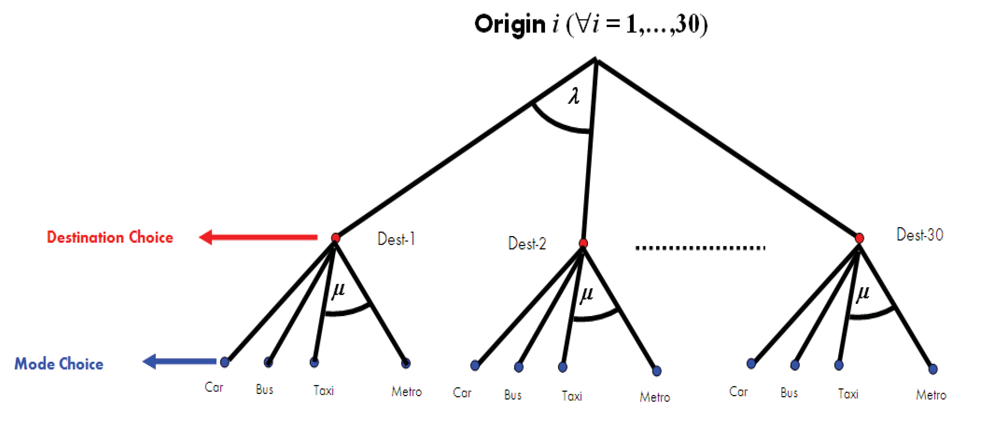
To compare the two parameter estimation approaches (ML and ME) we conducted a series of Monte Carlo simulations of a hierarchical model of combined destination choice and modal share using various sample sizes and values for the parameter μ. Although this HL model is particular, it illustrates clearly the differences between both approaches. The simulated tree structure is depicted in Figure 1.

Figure 1. Simulated hierarchical tree structure.

Figure 1. Simulated hierarchical tree structure.

We defined 30 origin and destination zones and four transportation modes (private car, bus, taxi and metro) available for trips between any origin and destination pair in either direction. For simplicity, we assumed that the parameter μ was the same for all destinations. The parameter $\lambda$ was set at unity ($\lambda =1$). No specific attributes were assumed for the different groups.

The utility functions for the four modes are given below. In each case, the explanatory variables are travel time and travel cost and we include mode constants:

$$V_{Car}={\beta }_{Car}^0+{\beta }^{Time}{T}_{Car}+{\beta }^{Cost}{C}_{Car}$$

(25)

$$V_{Bus}={\beta }_{Bus}^0+{\beta }^{Time}{T}_{Bus}+{\beta }^{Cost}{C}_{Bus}$$

(26)

$$V_{Taxi}={\beta }_{Taxi}^0+{\beta }^{Time}{T}_{Taxi}+{\beta }^{Cost}{C}_{Taxi}$$

(27)

$$V_{Metro}={\beta }_{Metro}^0+{\beta }^{Time}{T}_{Metro}+{\beta }^{Cost}{C}_{Metro}$$

(28)

The explanatory variable parameters are generic, that is, the same for each mode. The values of these population parameters are set out in Table 1.

Table 1. Population parameter values in simulations.

PARAMETER	VALUE (*)
${\beta }_{Car}^0$	0.9
${\beta }_{Bus}^0$	0
${\beta }_{Taxi}^0$	0.5
${\beta }_{Metro}^0$	0.4
${\beta }^{Time}$	−0.25
${\beta }^{Cost}$	−0.006
SVT (**)	41.47
λ	1
ϕ = λ/μ = 1/μ	0.5 (***)

(*) Values are defined by the authors, and are similar to the estimates reported in [21]; (**) Subjective value of time, estimated at (−0.25/−0.006) = 41.47; (***) Values of 0.2 and 0.9 were considered in complementary analysis, which is reported in the appendices.

Table 1. Population parameter values in simulations.

PARAMETER	VALUE (*)
${\beta }_{Car}^0$	0.9
${\beta }_{Bus}^0$	0
${\beta }_{Taxi}^0$	0.5
${\beta }_{Metro}^0$	0.4
${\beta }^{Time}$	−0.25
${\beta }^{Cost}$	−0.006
SVT (**)	41.47
λ	1
ϕ = λ/μ = 1/μ	0.5 (***)

(*) Values are defined by the authors, and are similar to the estimates reported in [21]; (**) Subjective value of time, estimated at (−0.25/−0.006) = 41.47; (***) Values of 0.2 and 0.9 were considered in complementary analysis, which is reported in the appendices.

The values for the explanatory variables (time and cost) were extracted from a 2001 transportation survey for Greater Santiago of Chile [23]. Their means and standard deviations for each transportation mode are given in Table 2.

A total of 1,000 Monte Carlo simulations were conducted with each of five different sample sizes containing 500, 1,000, 5,000, 10,000 and 20,000 observations, respectively. We thus obtained 1,000 ML and ME estimators of the parameters for each sample size, from which the estimates of bias, variance and mean squared error were derived.

The likelihood and entropy maximization problems were solved numerically using Newton’s method. The convergence criterion in all simulations was 0.1%, meaning that the percentage difference between the estimates of each parameter obtained from two consecutive iterations of the method did not exceed 0.001.

Table 2. Mean and standard deviation of explanatory variables by mode.

MODE	VARIABLE	MEAN (*)	STD DEV (*)
Car	Travel time	16	11
	Cost	2,031	138
Taxi	Travel time	17	11
	Cost	2,279	148
Bus	Travel time	54	12
	Cost	409	25
Metro	Travel time	45	7
	Cost	833	73

Source: [23]. (*) Travel time in minutes and cost in Chilean pesos as of 2009.

Table 2. Mean and standard deviation of explanatory variables by mode.

MODE	VARIABLE	MEAN (*)	STD DEV (*)
Car	Travel time	16	11
	Cost	2,031	138
Taxi	Travel time	17	11
	Cost	2,279	148
Bus	Travel time	54	12
	Cost	409	25
Metro	Travel time	45	7
	Cost	833	73

Source: [23]. (*) Travel time in minutes and cost in Chilean pesos as of 2009.

3.1. Bias, Variance and Mean Squared Error (MSE)

The 1,000 ML and ME estimators were used to construct histograms for simultaneously analyzing bias, variance and mean squared error. In Figure 2 we compare histograms of the observed modal split and modeled modal split for the maximum likelihood estimator, for three sample size (1,000, 5,000 and 10,000); in maximum entropy estimator, both observed and modeled modal split are identical by construction [see Equation (19)]. Each variable a was defined, for each simulations and mode a (car, taxi, bus and metro) by the following expression: ${\epsilon }_a={\displaystyle \sum _{gi}\left(p_{agi}-N_{agi}^0\right)/N_{agi}^0}$. We observe that, just asymptotically, modeled modal split converges to observed modal split [see Equation (15)].

Figure 2. Observed vs. modeled modal split using maximum likelihood estimation, for parameter value ϕ = 1/μ = 0.5.

Figure 2. Observed vs. modeled modal split using maximum likelihood estimation, for parameter value ϕ = 1/μ = 0.5.

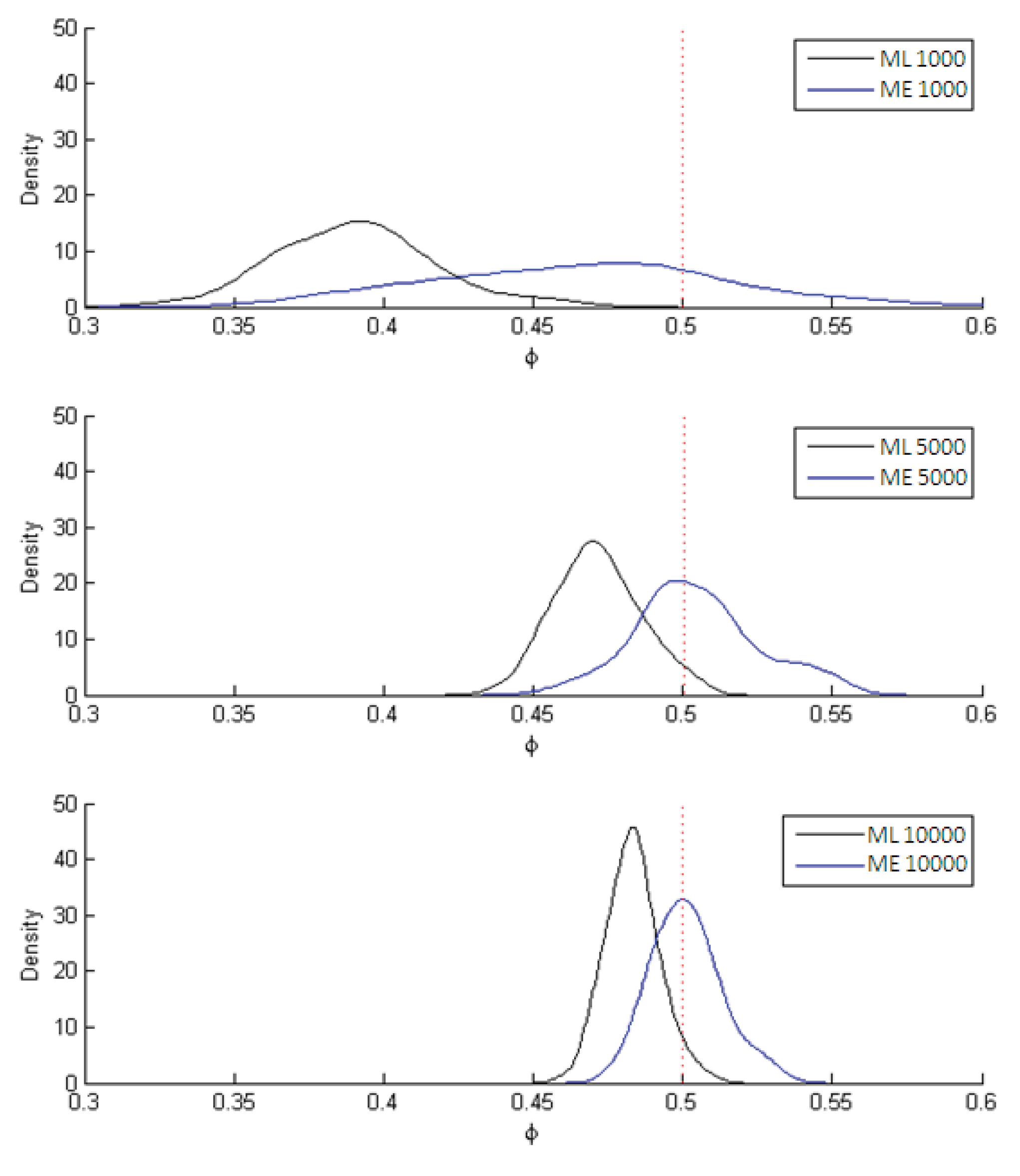
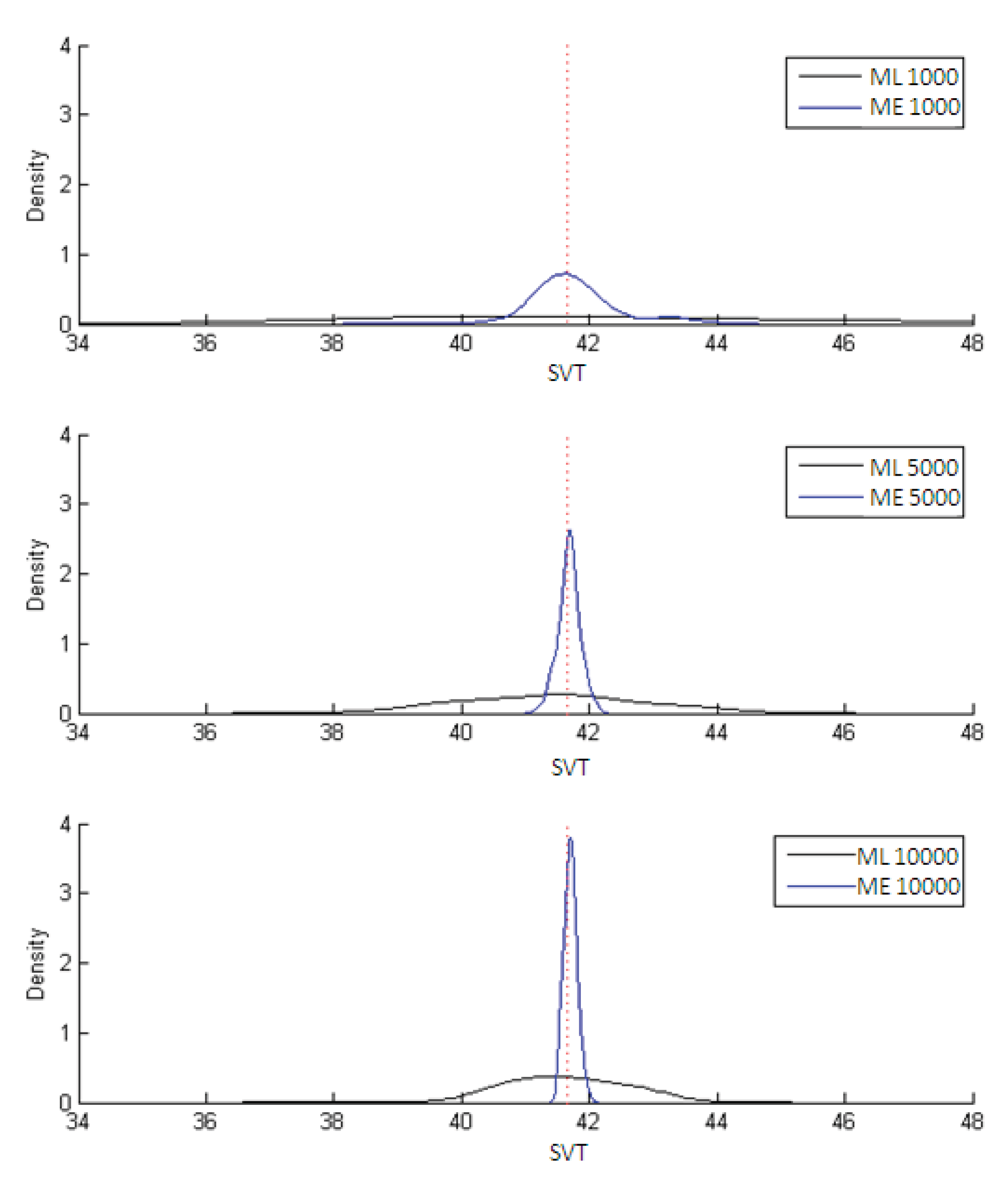
The estimates of the parameter ϕ = 1/μ are shown in Figure 3 while the estimates of the subjective value of time (SVT) are displayed in Figure 4. In both figures the dotted line marks the population parameter (used in the simulation) while the black curve traces out the ML estimates and the blue curve the ME estimates. The results in all cases are for 1,000; 5,000 and 10,000 observations, the three instances in which the differences between the two estimators most clearly stand out.

Figure 3. Results of ML and ME estimators for parameter value ϕ = 1/μ = 0.5.

Figure 3. Results of ML and ME estimators for parameter value ϕ = 1/μ = 0.5.

Figure 4. Results of ML and ME estimators for SVT = β^Time/β^Cost.

Figure 4. Results of ML and ME estimators for SVT = β^Time/β^Cost.

As can be seen in Figure 3, the ML estimate of μ is relatively biased but consistent while the ME estimate is significantly less biased but also less efficient (i.e., greater variance).

Figure 4 shows that both estimators of SVT are unbiased, although the ME estimator is clearly more efficient. This is confirmed in Table 3, which summarizes the results on bias, variance and MSE for both ML and ME. Also clear from the table is that the ME estimators are less biased than the ML ones, though the variances of the latter are smaller. The MSE, however, is always lower for the ME estimators.

Table 3. Summary of results for ML and ME estimators.

METHOD	PARAMETER	SAMPLE SIZE	BIAS	VARIANCE	MSE (*)
ML	1/μ	500	0.16844	0.00096	0.02933
	1/μ	1,000	0.10912	0.00074	0.01265
	1/μ	5,000	0.03067	0.00016	0.00110
	1/μ	10,000	0.01655	0.00009	0.00036
	1/μ	20,000	0.00821	0.00004	0.00011
	VST	500	2.57679	47.61970	54.25957
	VST	1,000	0.68741	13.87630	14.34884
	VST	5,000	0.16172	3.01595	3.04210
	VST	10,000	0.12386	1.23927	1.25461
	VST	20,000	0.11537	0.71021	0.72352
ME	1/μ	500	0.12867	0.00384	0.02039
	1/μ	1,000	0.03050	0.00250	0.00343
	1/μ	5,000	0.00494	0.00047	0.00050
	1/μ	10,000	0.00182	0.00017	0.00017
	1/μ	20,000	0.00023	0.00006	0.00006
	VST	500	1.70225	12.01048	14.90812
	VST	1,000	0.35554	1.95599	2.08240
	VST	5,000	0.19228	0.22072	0.25769
	VST	10,000	0.08879	0.07469	0.08257
	VST	20,000	0.03281	0.01565	0.01672

(*) Defined as the sum of the variance and the square of the bias.

Table 3. Summary of results for ML and ME estimators.

METHOD	PARAMETER	SAMPLE SIZE	BIAS	VARIANCE	MSE (*)
ML	1/μ	500	0.16844	0.00096	0.02933
	1/μ	1,000	0.10912	0.00074	0.01265
	1/μ	5,000	0.03067	0.00016	0.00110
	1/μ	10,000	0.01655	0.00009	0.00036
	1/μ	20,000	0.00821	0.00004	0.00011
	VST	500	2.57679	47.61970	54.25957
	VST	1,000	0.68741	13.87630	14.34884
	VST	5,000	0.16172	3.01595	3.04210
	VST	10,000	0.12386	1.23927	1.25461
	VST	20,000	0.11537	0.71021	0.72352
ME	1/μ	500	0.12867	0.00384	0.02039
	1/μ	1,000	0.03050	0.00250	0.00343
	1/μ	5,000	0.00494	0.00047	0.00050
	1/μ	10,000	0.00182	0.00017	0.00017
	1/μ	20,000	0.00023	0.00006	0.00006
	VST	500	1.70225	12.01048	14.90812
	VST	1,000	0.35554	1.95599	2.08240
	VST	5,000	0.19228	0.22072	0.25769
	VST	10,000	0.08879	0.07469	0.08257
	VST	20,000	0.03281	0.01565	0.01672

(*) Defined as the sum of the variance and the square of the bias.

For parameter values ϕ = 1/μ = 0.2 and ϕ = 1/μ = 0.9, the bias, variance and MSE estimates with the same sample sizes are found in Appendix B. In every case both bias and MSE are smaller for the ME estimator.

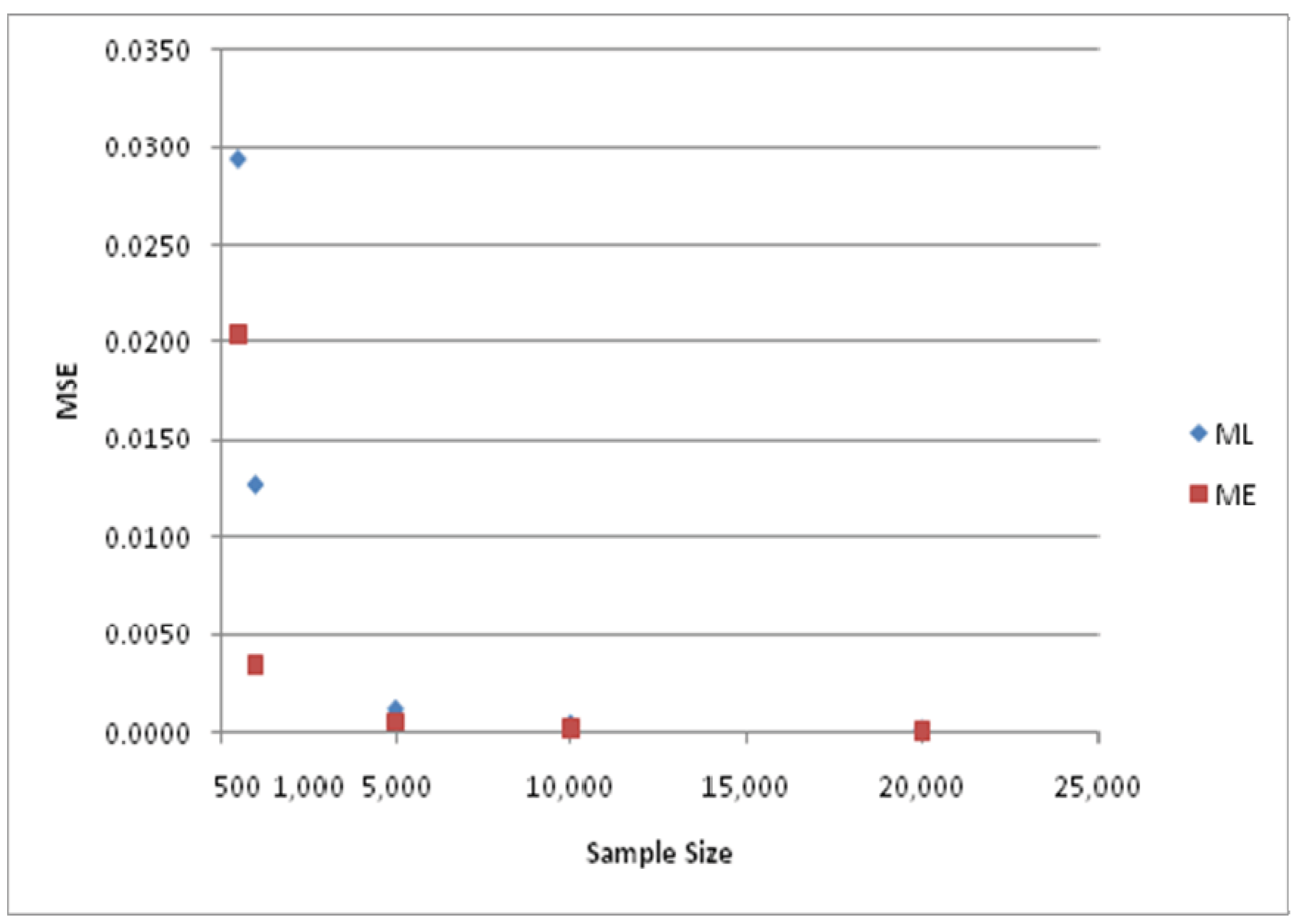
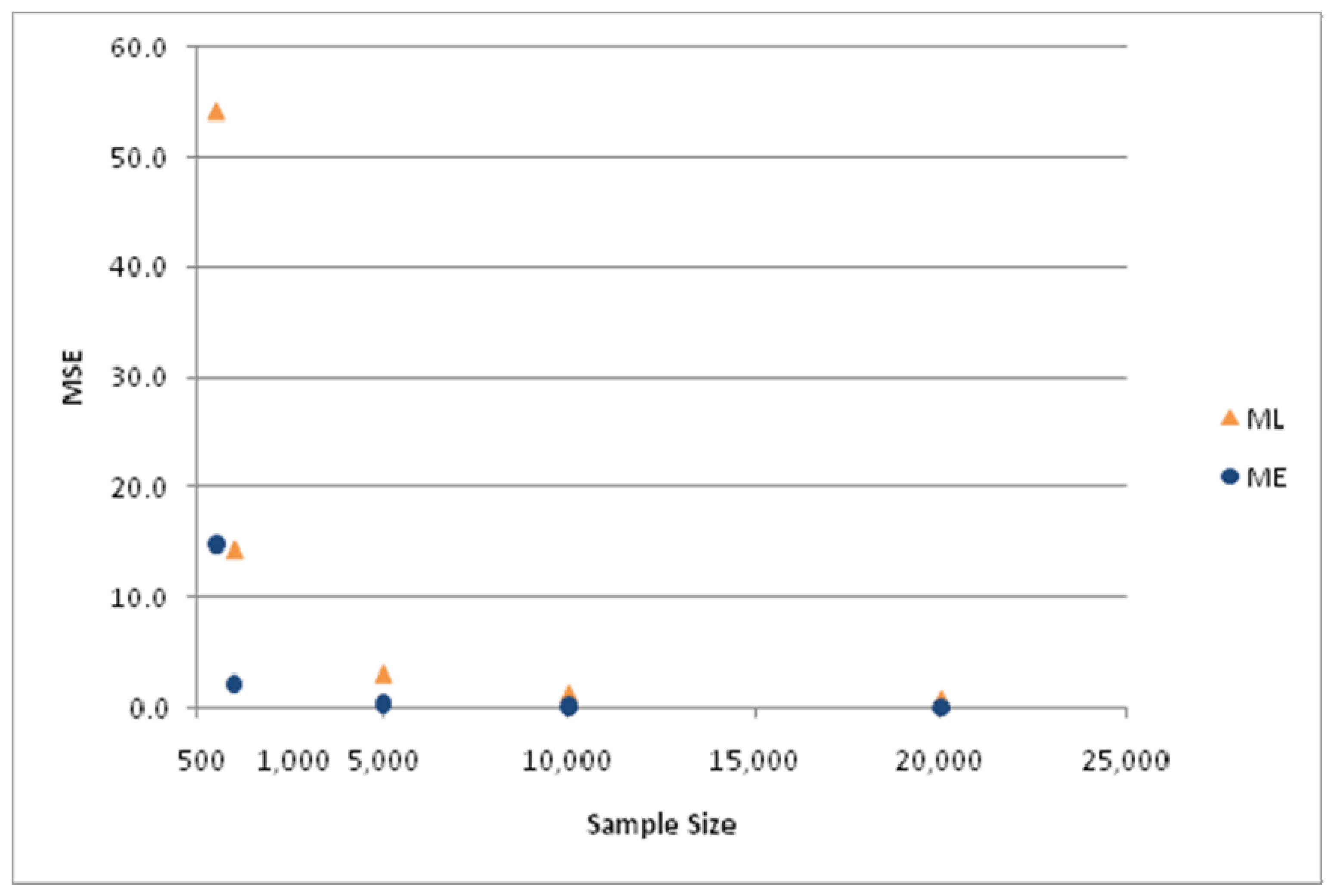
The differences in MSE for the two estimators are depicted in Figure 5 and Figure 6. The various results just presented lead to the conclusion that the ME estimator is systematically superior to the ML estimator in this hierarchical tree structure, particularly for small sample sizes.

The differences between both estimation approaches may respond to their abilities for reproducing the market modal shares of the calibration samples. It is well established that when the utility functions of a multinomial model contain a constant term by mode the modeled and observed modal shares are always the same [24]. This is not the case for the hierarchical logit model when its parameters are estimated by ML. Under the ME approach, however, the problem constraints force the market modal shares to be reproduced.

Figure 5. MSE of ML and ME estimators for parameter value ϕ = 1/μ = 0.5.

Figure 5. MSE of ML and ME estimators for parameter value ϕ = 1/μ = 0.5.

Figure 6. MSE of ML and ME estimators for SVT.

Figure 6. MSE of ML and ME estimators for SVT.

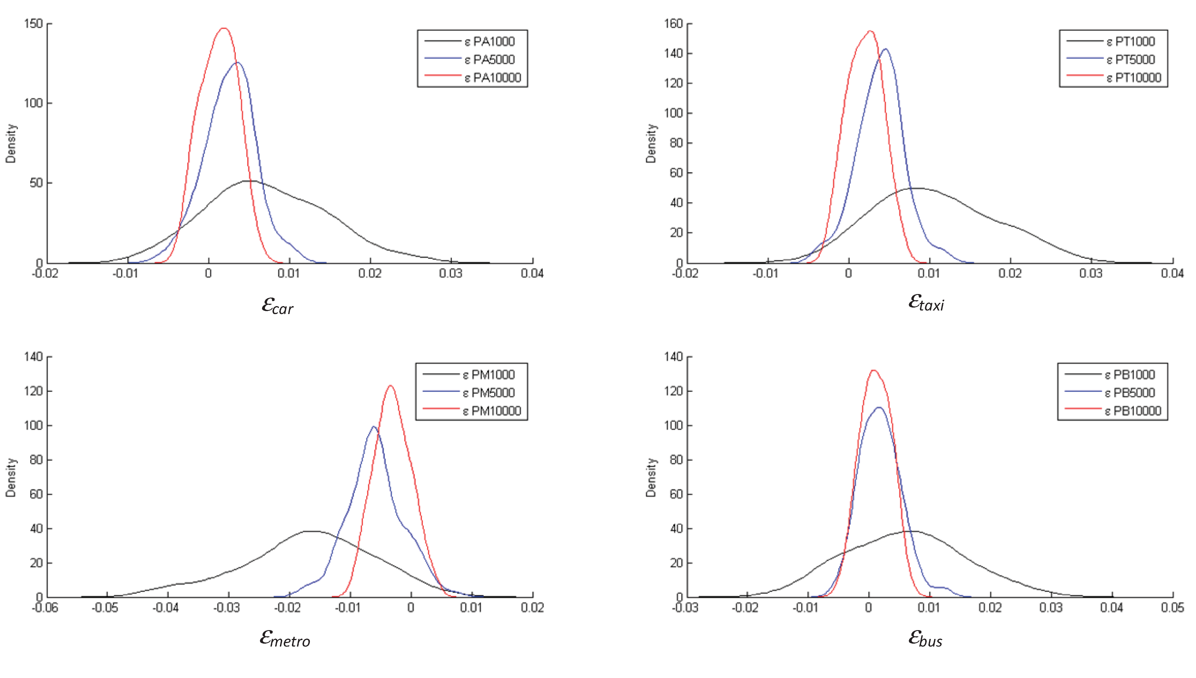
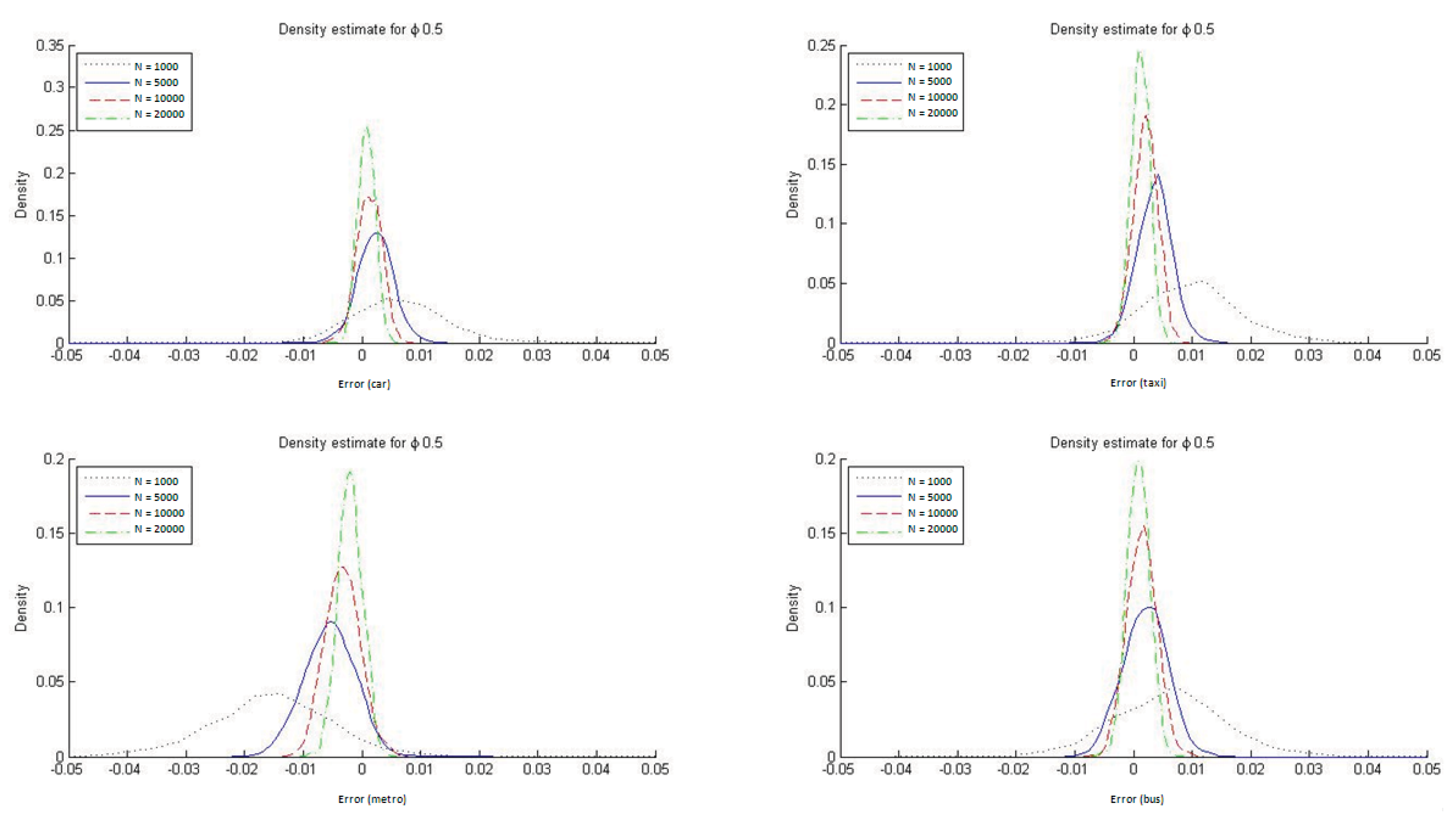
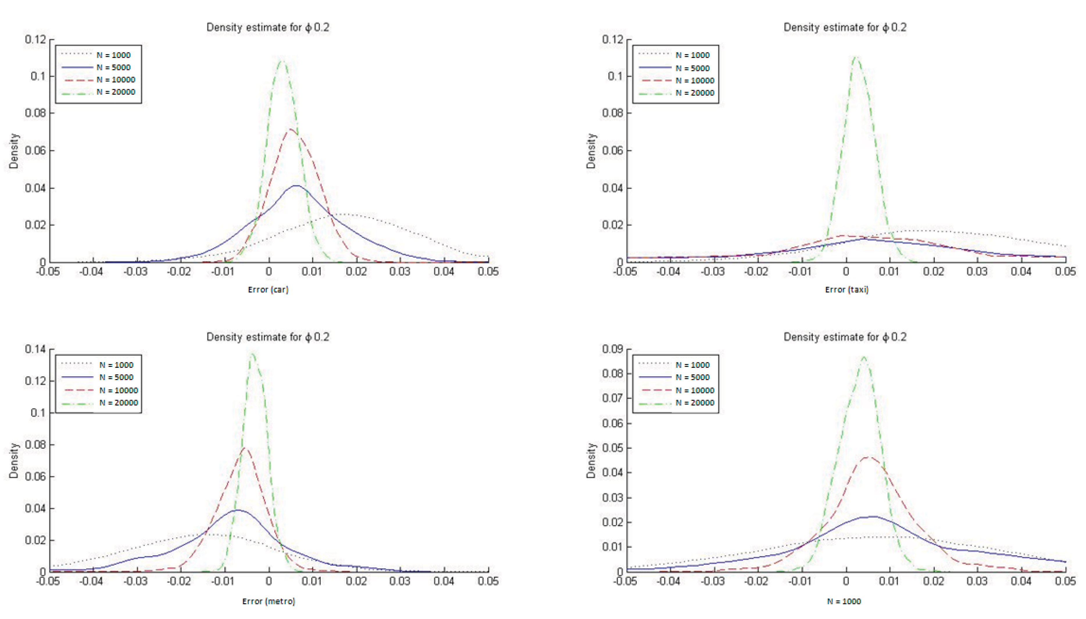
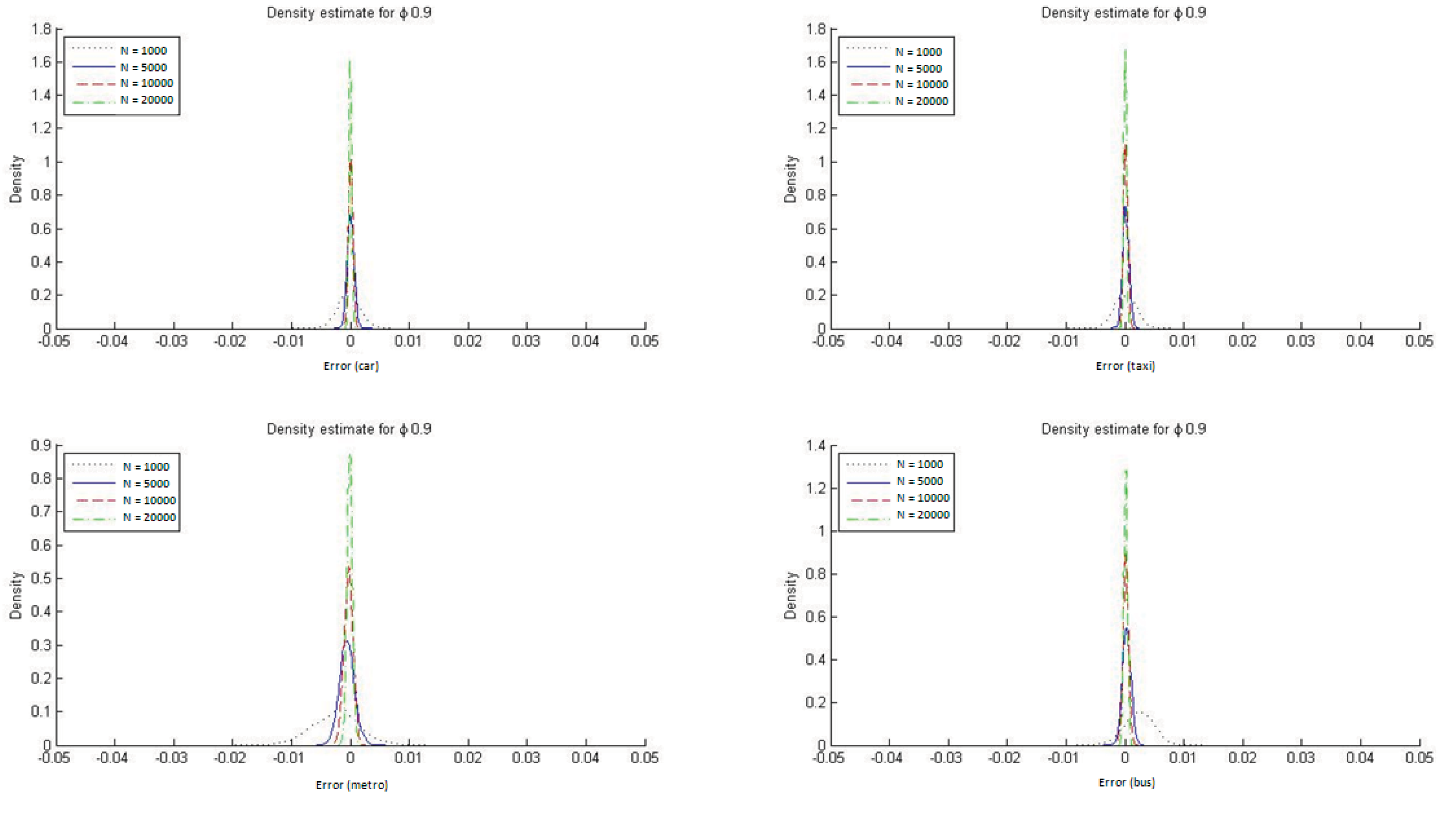
To determine the ability of the ML estimators to reproduce the market modal shares in HL models, we constructed histograms of DMS, defined as the difference between the modeled and observed modal shares (see Figure 7). These differences were estimated for each of the four transportation modes. As is apparent from the figure, the ML estimators of the hierarchical logit model do not, on average, reproduce the sample modal shares, particularly in small samples.

It is also evident from Figure 7 that with HL models the ML estimator reproduces the market modal shares only asymptotically whereas by construction the ME estimators always reproduce them. In Appendix C we report the DMS distributions for the four transportation modes when ϕ = 1/μ = 0.2 and ϕ = 1/μ = 0.9. The conclusions are similar for the two cases, but with ϕ = 1/μ = 0.9 it is especially clear that the ML estimate for the HL model reproduces the modal shares must more accurately. This result is to be expected given that a value for the parameter ϕ closer to 1 implies that the HL model is more similar to an MNL one, which always reproduces the observed modal shares when estimated with ML.

Figure 7. Distribution of DMS with ML estimation (ϕ = 1/μ = 0.5).

Figure 7. Distribution of DMS with ML estimation (ϕ = 1/μ = 0.5).

3.2. Estimate of Consumer Surplus

Also of interest is the comparison of the ML and ME estimates of consumer surplus generated by our combined destination and mode choice model. This measure of the welfare perceived by the transportation system user is expressed by the expected maximum utility (EMU), which is written as follows:

$$-{\displaystyle \sum _{a,g,i}{N}_i^0{p}_{ag/i}ln{p}_{ag/i}}=-{\displaystyle \sum _{i,g}{N}_i^0{p}_{g/i}ln{p}_{g/i}}-{\displaystyle \sum _{a,g,i}{N}_i^0{p}_{g/i}{p}_{a/gi}ln{p}_{a/gi}}$$

(29)

This expression gives the consumer surplus of individual i in group g. The group refers to the origin-destination pair representing the trip taken, and since our model is an aggregate one, all individuals in a given group have the same utility function $V_{agi}$ for each mode alternative a. This being the case, we have EMU_gi = EMU_g, and can therefore estimate the average EMU as:

$$EM{U}_{average}=\frac{{\displaystyle \sum _{a,g}{t}_{ag}EM{U}_g}}{{\displaystyle \sum _{a,g}{t}_{ag}}}$$

(30)

where t_ag is the number of individuals in group g that takes alternative a. We will use average EMU to make comparisons with the results generated by the simulations for various sample sizes (the sum of the t_ag will therefore equal the size of the sample from which the parameters that give the EMU are estimated).

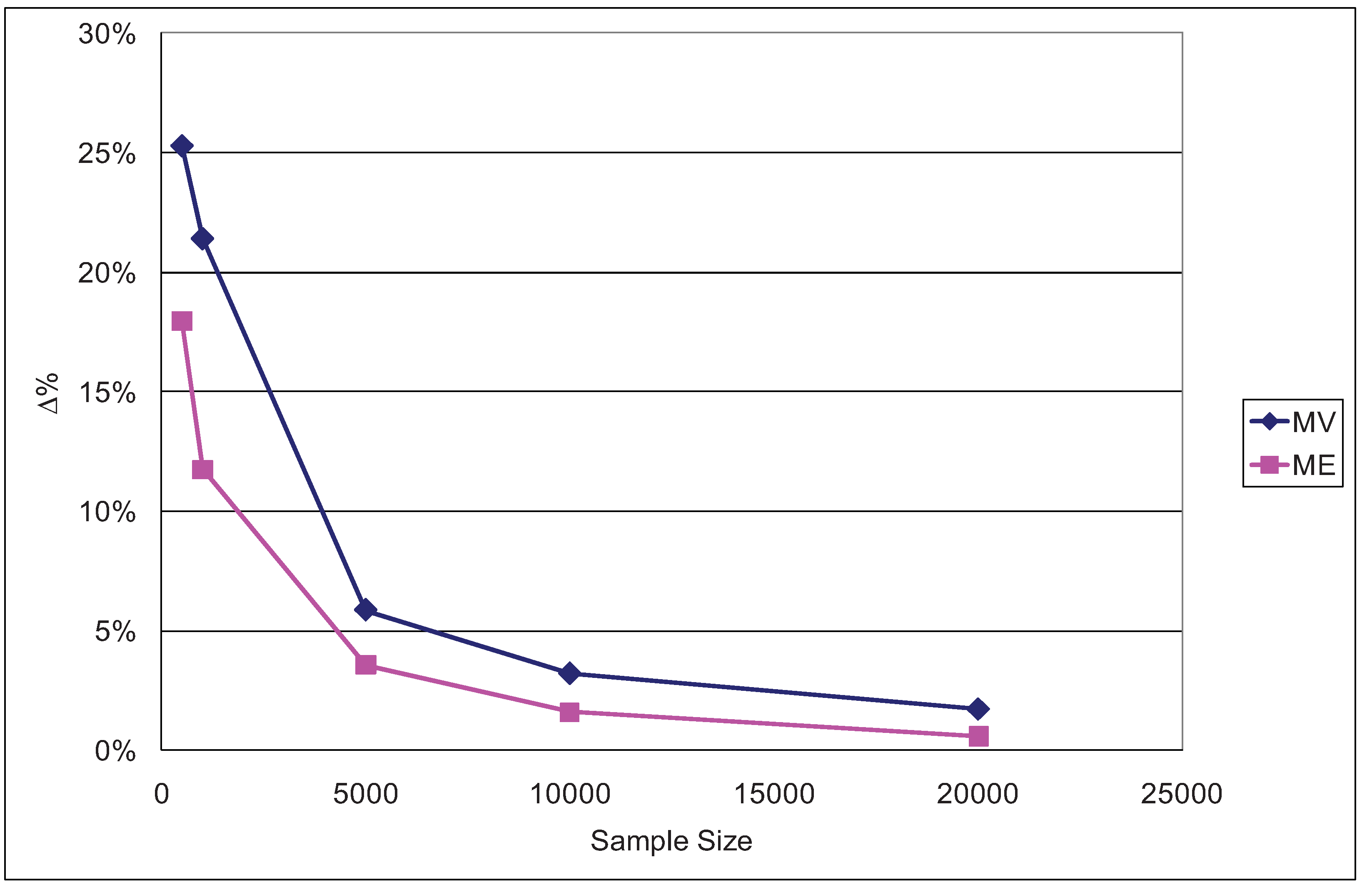
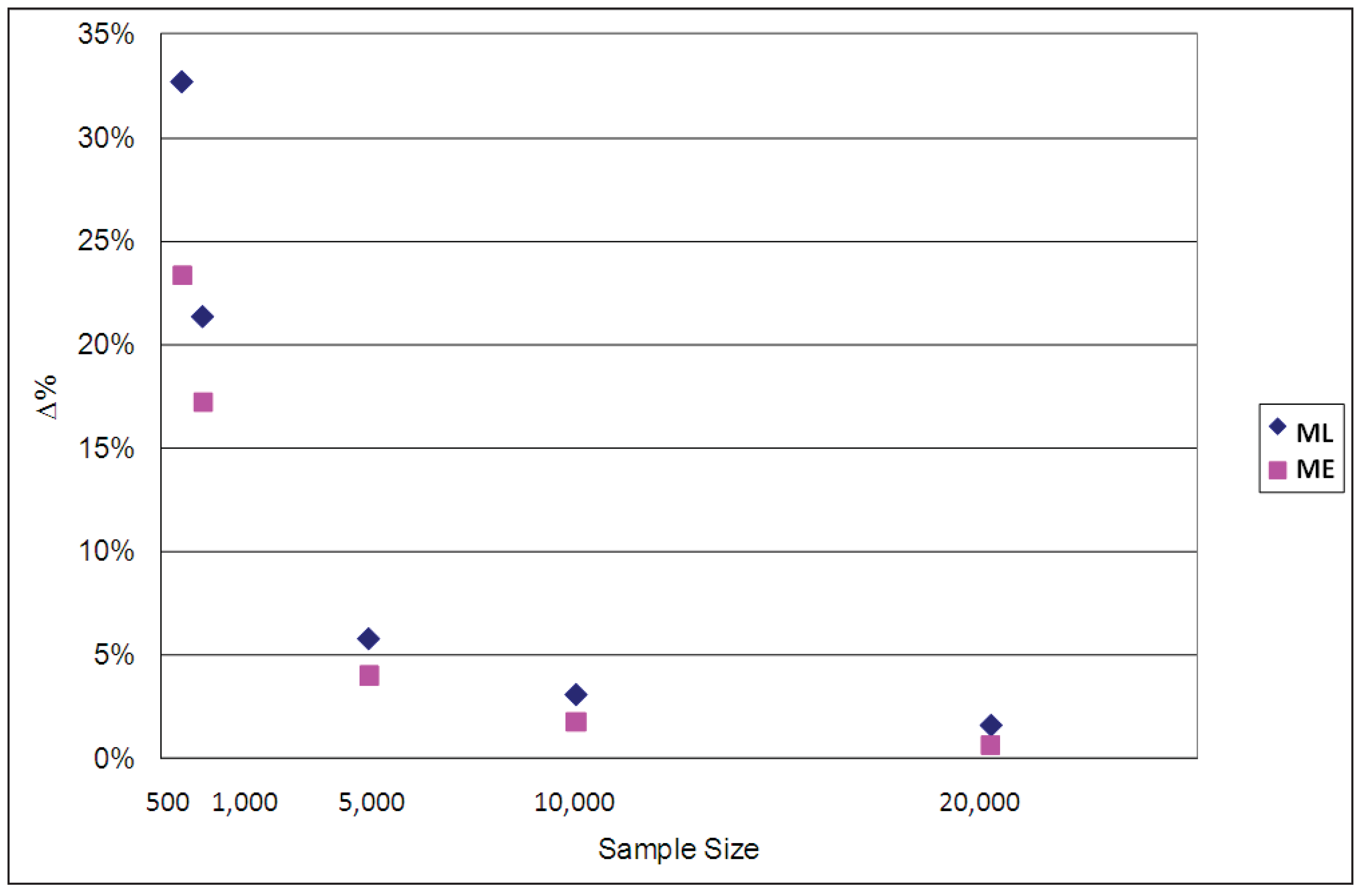
The average EMU values estimated for each case using the ML and ME estimators are compared with the population parameters used for the simulations in Table 4. The percentage differences between the estimated and population parameter values are graphed in Figure 8. It is clear from both the table and the figure that the EMU estimates produced by the ML parameters are more biased than those of the ME parameters, especially when sample sizes are small, though they both converge asymptotically to the true values when the sample size increases. The corresponding results for ϕ = 1/μ = 0.2 and ϕ = 1/μ = 0.9 are reported in Appendix D, confirming that for all three cases (ϕ = 0.2, ϕ = 0.5 and ϕ = 0.9) the ME estimator of average EMU is less biased than the ML one.

Table 4. Average EMU.

SAMPLE SIZE	SIMULATION	ML	Δ% ML (*)	ME	Δ% ME (*)
500	7.0574	4.7481	32.7%	5.4107	23.3%
1,000	7.0601	5.5514	21.4%	5.8450	17.2%
5,000	7.0918	6.6807	5.8%	6.8073	4.0%
10,000	7.0755	6.8564	3.1%	6.9500	1.8%
20,000	7.0679	6.9539	1.6%	7.0223	0.6%

(*) Calculated as the difference between population (simulation) and estimated EMU divided by population EMU.

Table 4. Average EMU.

SAMPLE SIZE	SIMULATION	ML	Δ% ML (*)	ME	Δ% ME (*)
500	7.0574	4.7481	32.7%	5.4107	23.3%
1,000	7.0601	5.5514	21.4%	5.8450	17.2%
5,000	7.0918	6.6807	5.8%	6.8073	4.0%
10,000	7.0755	6.8564	3.1%	6.9500	1.8%
20,000	7.0679	6.9539	1.6%	7.0223	0.6%

(*) Calculated as the difference between population (simulation) and estimated EMU divided by population EMU.

Figure 8. Percentage differences between population and estimated average EMU (ϕ = 1/μ = 0.5).

Figure 8. Percentage differences between population and estimated average EMU (ϕ = 1/μ = 0.5).

3.3. Out-of-Sample Prediction

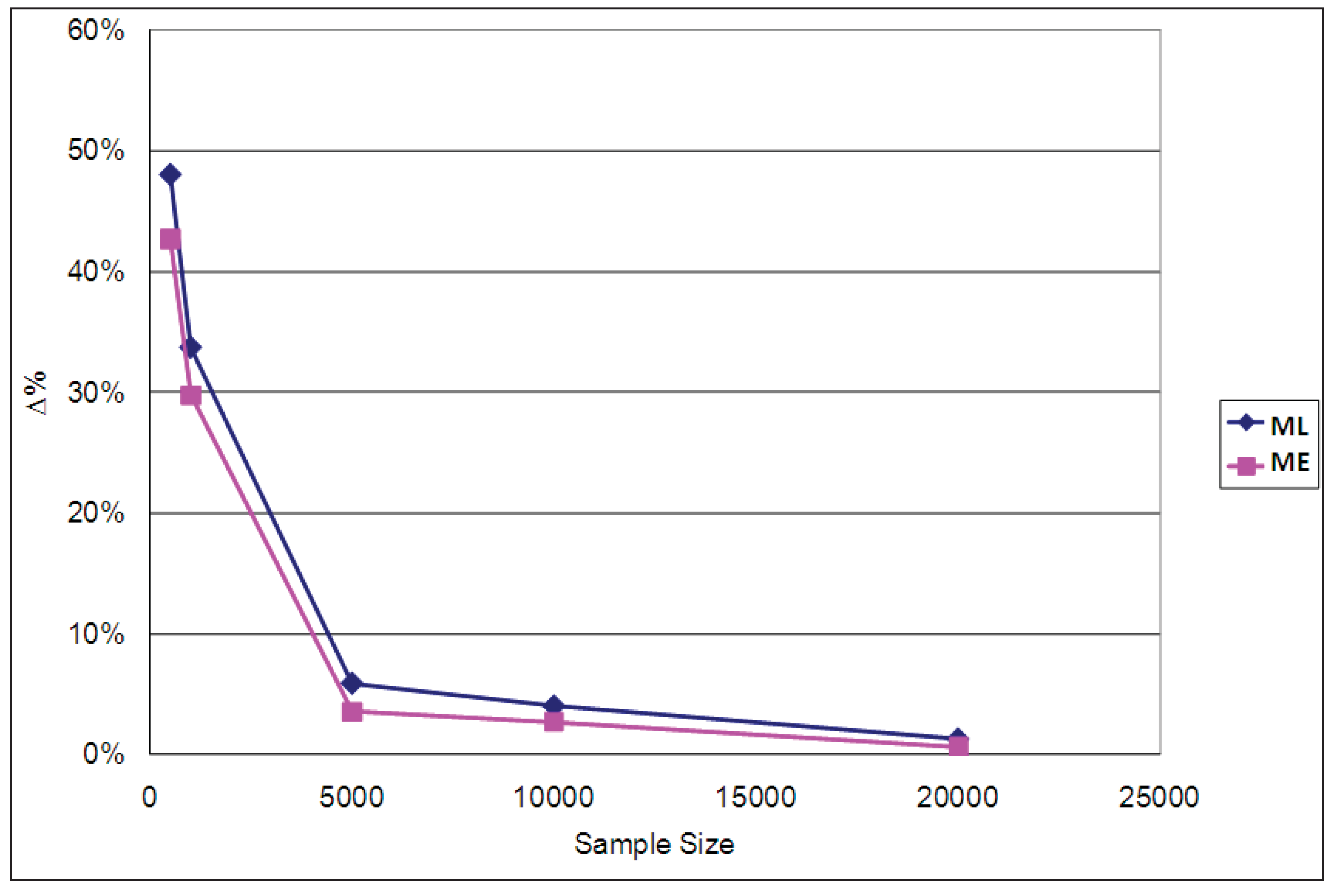
To study the behavior of the ML and ME estimators of consumer surplus we varied the travel times of the four transportation modes and estimated the resulting changes in average EMU as given by (13). The travel time variations consisted in reducing this factor by 10% for all four modes. The results obtained are shown for various sample sizes in Figure 9.

Figure 9. Percentage differences in ΔEMU for a 10% reduction in travel time (ϕ = 1/μ = 0.5).

Figure 9. Percentage differences in ΔEMU for a 10% reduction in travel time (ϕ = 1/μ = 0.5).

In every case it can be observed that the ML overestimates EMU to a greater extent than does ME. The overestimation effect is particularly significant for the small samples (500 and 1,000 data items), which is consistent with Figure 9. The corresponding results for ϕ = 1/μ = 0.2 and ϕ = 1/μ = 0.9 are reported in Appendix E, confirming that for all three cases (ϕ = 0.2, ϕ = 0.5 and ϕ = 0.9) the ME overestimate of ΔEMU is smaller than the ML one.

4. Conclusions

In the context of aggregate transportation demand forecasting and land use planning, entropy maximization problems are often formulated, mainly because their solutions are the well-known multinomial logit and hierarchical logit models. The parameters of these models are normally estimated using the maximum likelihood method, but they can also be estimated by solving the entropy maximization problems directly. These latter estimators are referred to here as maximum entropy estimators. It has long been known (see [1,22]) that both estimation methods lead to the same results if the model is multinomial logit.

This work extended the analysis to the case of aggregate hierarchical logit models. We began by formulating a general problem of maximizing the hierarchical entropy and deducing that its solution is a hierarchical logit model. We then observed that the maximum entropy estimators were different from the maximum likelihood ones, especially in that the latter do not reproduce either the average values of the explanatory variables or the observed market modal shares (of the calibration sample) whereas the maximum entropy estimators do reproduce them by construction.

The two estimators were then subjected to various empirical analyses. The population parameters of a relatively general travel demand hierarchical model were estimated using Monte Carlo simulations with samples of various sizes. The results obtained showed that the maximum entropy estimator is superior to the maximum likelihood estimator, especially for smaller sample sizes. More specifically, the maximum entropy estimator exhibited less bias and a smaller mean square error. The reduced bias in turn results in underestimations of consumer surplus with maximum likelihood.

Though similar analyses of other hierarchical structures are required, we may conclude on the basis of the results presented here that the maximum entropy approach is a better alternative for estimating hierarchical logit aggregate models than the maximum likelihood approach, particularly with small or medium-size samples such as those typically used in actual transportation planning processes.

References

1. Anas, A. Discrete choice theory, information theory and the multinomial logit and gravity models. Transp. Res. 1983, 17, 13–23. [Google Scholar] [CrossRef]
2. Williams, H.C.W.L. On the formation of travel demand models and economic evaluation measures of user benefit. Environ. Plan. 1977, 9, 285–344. [Google Scholar] [CrossRef]
3. Wilson, A.G. Entropy in Urban and Regional Modeling; Pion: London, UK, 1970. [Google Scholar]
4. Morrison, W.; Thumann, R. Lagrangian multiplier approach to the solution of a special constrained matrix problem. J. Reg. Sci. 1980, 20, 279–292. [Google Scholar] [CrossRef]
5. Fotheringham, A. A new set of spatial interaction models: The theory of competing destinations. Environ. Plan. 1983, 15A, 15–36. [Google Scholar] [CrossRef]
6. Fotheringham, A. Modeling hierarchical destination choice. Environ. Plan. 1986, 18, 401–418. [Google Scholar] [CrossRef]
7. Fang, S.; Tsao, J. Linearly-constrained entropy maximization problem with quadratic cost and its applications to transportation planning problems. Transp. Sci. 1995, 29, 353–365. [Google Scholar] [CrossRef]
8. Thorsen, I.; Gitlesen, J.P. Empirical evaluation of alternative model specifications to predict commuting flows. J. Reg. Sci. 1998, 38, 273–292. [Google Scholar] [CrossRef]
9. De Grange, L; Ibeas, A; Gonzalez, F. A hierarchical gravity model with spatial correlation: Mathematical formulation and parameter estimation. Netw. Spat. Econ. 2009. [Google Scholar] [CrossRef]
10. De Grange, L.; Fernandez, J.E.; De Cea, J. A consolidated model of trip distribution. Transp. Res. 2010, 46, 61–75. [Google Scholar] [CrossRef]
11. Boyce, D.; LeBlanc, L.; Chon, K.; Lee, Y.; Lin, K. Implementation and computational issues for combined models of location, destination, mode and route choice. Environ. Plan. 1983, 15, 1219–1230. [Google Scholar] [CrossRef]
12. Boyce, D.; LeBlanc, L.; Chon, K. Network equilibrium models of urban location and travel choices: A retrospective survey. J. Reg. Sci. 1988, 28, 159–183. [Google Scholar] [CrossRef]
13. Safwat, K.; Magnanti, T. A combined trip generation, trip distribution, modal split and traffic assignment model. Transp. Sci. 1988, 22, 14–30. [Google Scholar] [CrossRef]
14. Brice, S. Derivation of nested transport models within a mathematical programming framework. Transp. Res. 1989, 23, 19–28. [Google Scholar] [CrossRef]
15. Fernandez, J.E.; De Cea, J.; Florian, M.; Cabrera, E. Network equilibrium models with combined modes. Transp. Sci. 1994, 28, 182–192. [Google Scholar] [CrossRef]
16. Oppenheim, N. Urban Travel Demand Modeling; John Wiley & Sons: New York, NY, USA, 1995. [Google Scholar]
17. Abrahamsson, T.; Lundqvist, L. Formulation and estimation of combined network equilibrium models with applications to stockholm. Transp. Sci. 1999, 33, 80–100. [Google Scholar] [CrossRef]
18. Boyce, D.; Bar-Gera, H. Validation of multiclass urban travel forecasting models combining origin-destination, mode, and route choices. J. Reg. Sci. 2003, 43, 517–540. [Google Scholar] [CrossRef]
19. Ham, H.; Tschangho, J.; Boyce, D. Implementation and estimation of a combined model of interregional, multimodal commodity shipments and transportation network flows. Transp. Res. 2005, 39, 65–79. [Google Scholar] [CrossRef]
20. Garcia, R.; Marin, A. Network equilibrium with combined modes: Models and solution algorithms. Transp. Res. 2005, 39, 223–254. [Google Scholar] [CrossRef]
21. De Cea, J.; Fernandez, J.E.; De Grange, L. Combined models with hierarchical demand choices: A multi-objective entropy optimization approach. Transp. Rev. 2008, 28, 415–438. [Google Scholar] [CrossRef]
22. Donoso, P.; De Grange, L. A Microeconomic interpretation of the maximum entropy estimator of multinomial logit models and its equivalence to the maximum likelihood estimator. Entropy 2010, 12, 2077–2084. [Google Scholar] [CrossRef]
23. SECTRA. Encuesta Origen Destino de Viajes 2001 para el Gran Santiago. Secretaría Interministerial de Planificación de Transporte, 2002, Santiago de Chile. Available online: http://www.sectra.cl/transporte/transporte_urbano_eod_frm.html (accessed on 21 March 2010).
24. Ortuzar, J.d.D.; Willumsen, L.G. Modeling Transport; John Wiley & Sons: Chichester, UK, 2001. [Google Scholar]
Appendices
Appendix A: Microeconomic Interpretation of the Entropy Maximization Dual Problem
The expected maximum utility (EMUi) of an individual i under a hierarchical logit choice structure is given by
E M U i = ln g / i exp ( V g i + V g i ) ,   V g i = 1 μ g ln ( a / g , i exp ( μ g V a g i ) )  for all  g , i
For the hierarchical logit model, it is known that
p a g / i = p a / g i p g / i = exp ( μ g V a g i ) a exp ( μ g V a g i ) exp ( V g i + V g i ) g exp ( V g i + V g i )
Since p g / i = exp ( V g i + V g i ) g exp ( V g i + V g i ) , we have
g exp ( V g i + V g i ) = exp ( V g i + V g i ) p g / i
ln ( g exp ( V g i + V g i ) ) = V g i + V g i ln p g / i = E M U i
Multiplying (33) by p g / i and then summing over g, we obtain
p g / i E M U i = p g / i ( V g i + V g i ) p g / i ln p g / i / g
E M U i = g / i p g / i ( V g i + V g i ) g / i p g / i ln p g / i
Since by (31) and (32), V g i = 1 μ g ln ( a / g , i exp ( μ g V a g i ) ) and p a / g i = exp ( μ g V a g i ) a exp ( μ g V a g i ) , we easily get
V g i = V a g i 1 μ g ln p a / g i p a / g i V g i = p a / g i V a g i p a / g i 1 μ g ln p a / g i / a / g , i
V g i = a / g , i p a / g i V a g i 1 μ g a / g , i p a / g i ln p a / g i
Finally, substituting (38) into (36) we obtain
E M U i = g / i p g / i ( a / g p a / g i V a g i 1 μ g a / g p a / g i ln p a / g i + V g i ) g / i p g / i ln p g / i
E M U i = g / i p g / i ( a / g p a / g i V a g i ) + g / i p g / i V g i g / i 1 μ g p g / i ( a / g , i p a / g i ln p a / g i ) g / i p g / i ln p g / i
Based on (40) we can now formulate the following optimization problem that each individual must solve:
max { p a / g i , p g / i } g / i p g / i ( a / g p a / g i V a g i ) + g / i p g / i V g i g / i 1 μ g p g / i ( a / g , i p a / g i ln p a / g i ) g / i p g / i ln p g / i s . t . :    a / g , i p a / g i = 1     for all  g , i      ( Φ g i )           g / i p g / i = 1      for all  i         ( γ i )
The optimality conditions for (41) are then
p a / g i = exp ( μ g V a g i ) a exp ( μ g V a g i ) ,          Φ g i = p g / i [ 1 μ g ln a / g , i exp ( μ g V a g i ) + 1 ]
p g / i = exp ( V g i + V g i ) g exp ( V g i + V g i ) ,          γ i = ln g / i exp ( V g i )
Assuming a linear and additive utility function V a g i = k β k x a g i k for each individual, and given that multiple individuals make their optimal decision (based on mixes strategies) simultaneously, we demonstrate that the optimization problem (41) is the equivalent problem of the optimization problem formulated in Section 2.3. Therefore, the value of the objective function of the latter problem at the optimum is the sum over all individuals of their maximum expected utilities from the available alternatives.
Appendix B: Estimates of Bias, Variance and Mean Square Error for Parameter Values ϕ = 1/μ = 0.2 and ϕ = 1/μ = 0.9