3. Results and Discussion
The results for the integration of the equations for the wave numbers represent the conservation of mass in the overall set of equations.
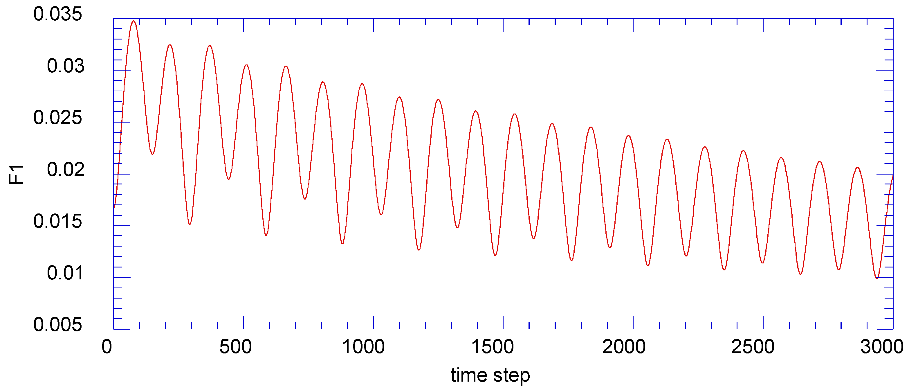
Figure 2 presents the perturbation factor
as a function of time step through the first portion the overall time range. These results show the periodic behavior for the forcing function. Note that this forcing function is internal to the set of six equations describing the overall flow, but represent an externally applied forcing function for the three equations describing the equations of motion.
Figure 2.
The periodic internal driving force obtained from the solution for the wave vectors from the continuity equations for an area ratio
Figure 2.
The periodic internal driving force obtained from the solution for the wave vectors from the continuity equations for an area ratio
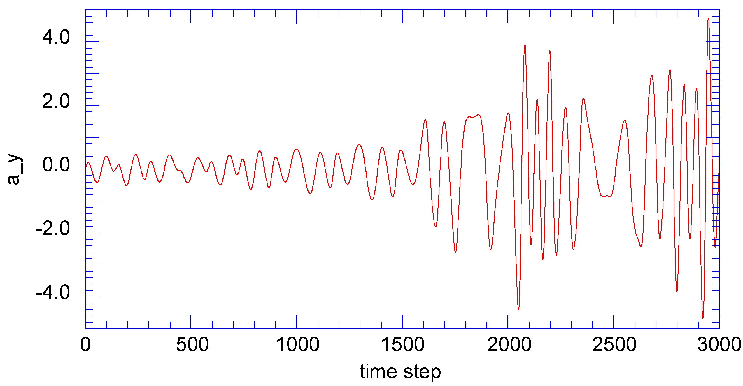
Figure 3 indicates the behavior of the vertical velocity component,
, with a moderate aperiodic behavior in the first part of the time series, with a transition to significant oscillations in the next part of the time series.
Figure 3.
The vertical component of the fluctuating velocity as a function of the time step for an area ratio
Figure 3.
The vertical component of the fluctuating velocity as a function of the time step for an area ratio
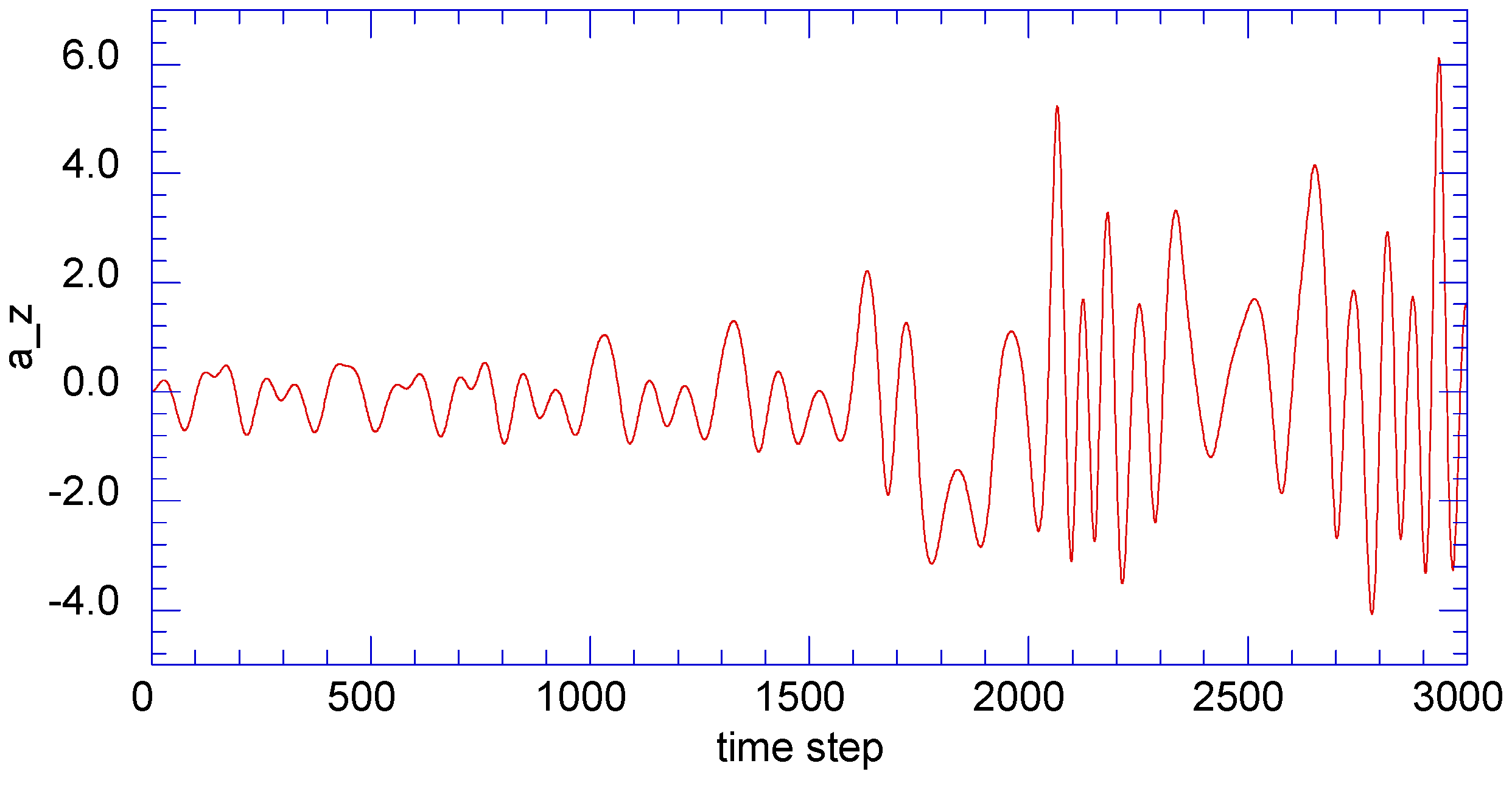
Figure 4 presents the time series for the span-wise component,
, which also represents this type of behavior. The span-wise fluctuating velocity component also indicates a transition to a significant level of oscillations, thus indicating the possible creation of ordered structures in the y-z plane in this region of the time series.
Figure 4.
The span-wise component of the fluctuating velocity as a function of the time step for an area ratio
Figure 4.
The span-wise component of the fluctuating velocity as a function of the time step for an area ratio
It is interesting to note that Prichard and Theiler [
30], in a study of the behavior of the Rössler attractor, observed that the local entropy is apparently large when the particular parameter is large. We, however, find that the spectral entropy is dependent on the degree of order within the flow element, with lower values of the spectral entropy representing a higher degree of order within the element. The spectral entropy does not seem to be dependent on the magnitude of the respective fluctuating velocity components, but rather increases as the degree of disorder increases.
Figure 5 presents the phase plane plot of the vertical component of velocity,
,
versus the axial velocity component,
, over the initial time frame of 1,000 time steps. The portion of the results on the right-hand side of the figure represents a Duffing-like equation behavior (Lynch [
31]), indicating a close coupling between the axial velocity component and the vertical velocity component. Then, the vertical velocity component accelerates to a constant velocity, as the axial velocity component decrease. This would indicate an almost organized motion of the system in the vertical direction.
Figure 5.
The phase plane representation of the vertical fluctuating velocity against the horizontal fluctuating velocity over 1,000 time steps for an area ratio
Figure 5.
The phase plane representation of the vertical fluctuating velocity against the horizontal fluctuating velocity over 1,000 time steps for an area ratio
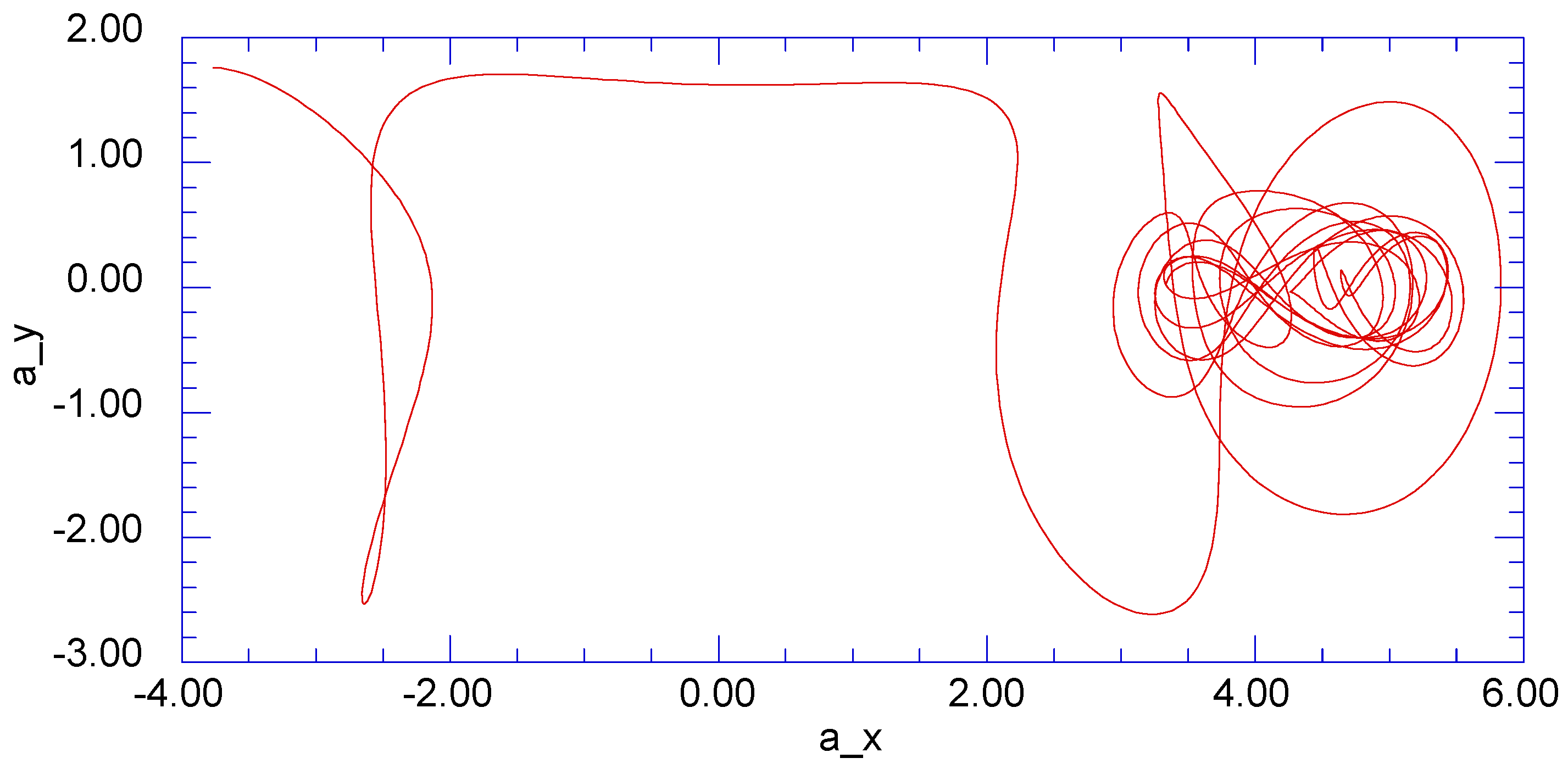
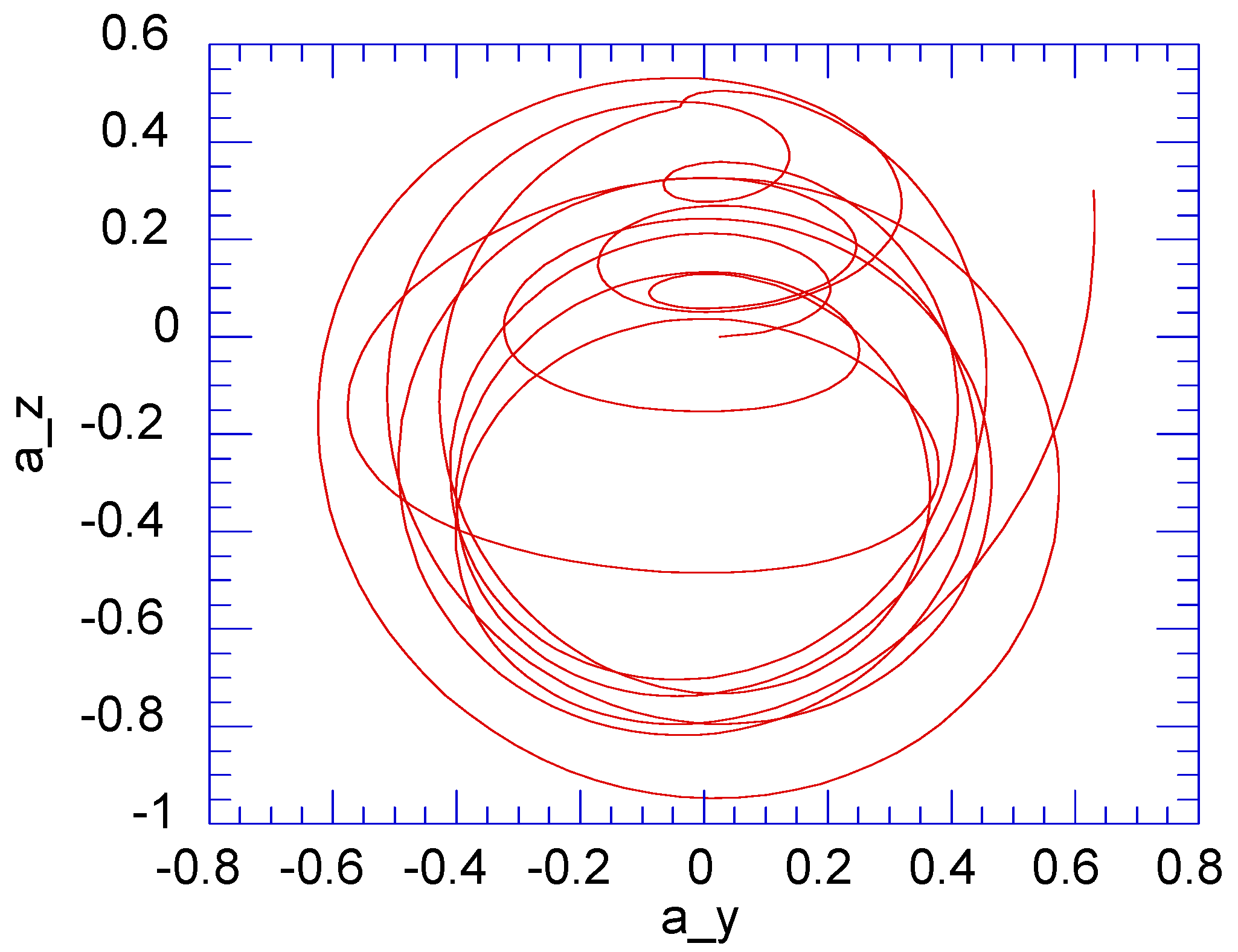
Figure 6 presents the phase plane results for the span-wise velocity component,
,
versus the vertical velocity component,
, which indicates a nearly periodic rotational behavior in the vertical and span-wise plane.
Figure 6.
The phase plane representation of the span-wise velocity fluctuations against the vertical velocity fluctuations over 1,000 time steps for an area ratio
Figure 6.
The phase plane representation of the span-wise velocity fluctuations against the vertical velocity fluctuations over 1,000 time steps for an area ratio
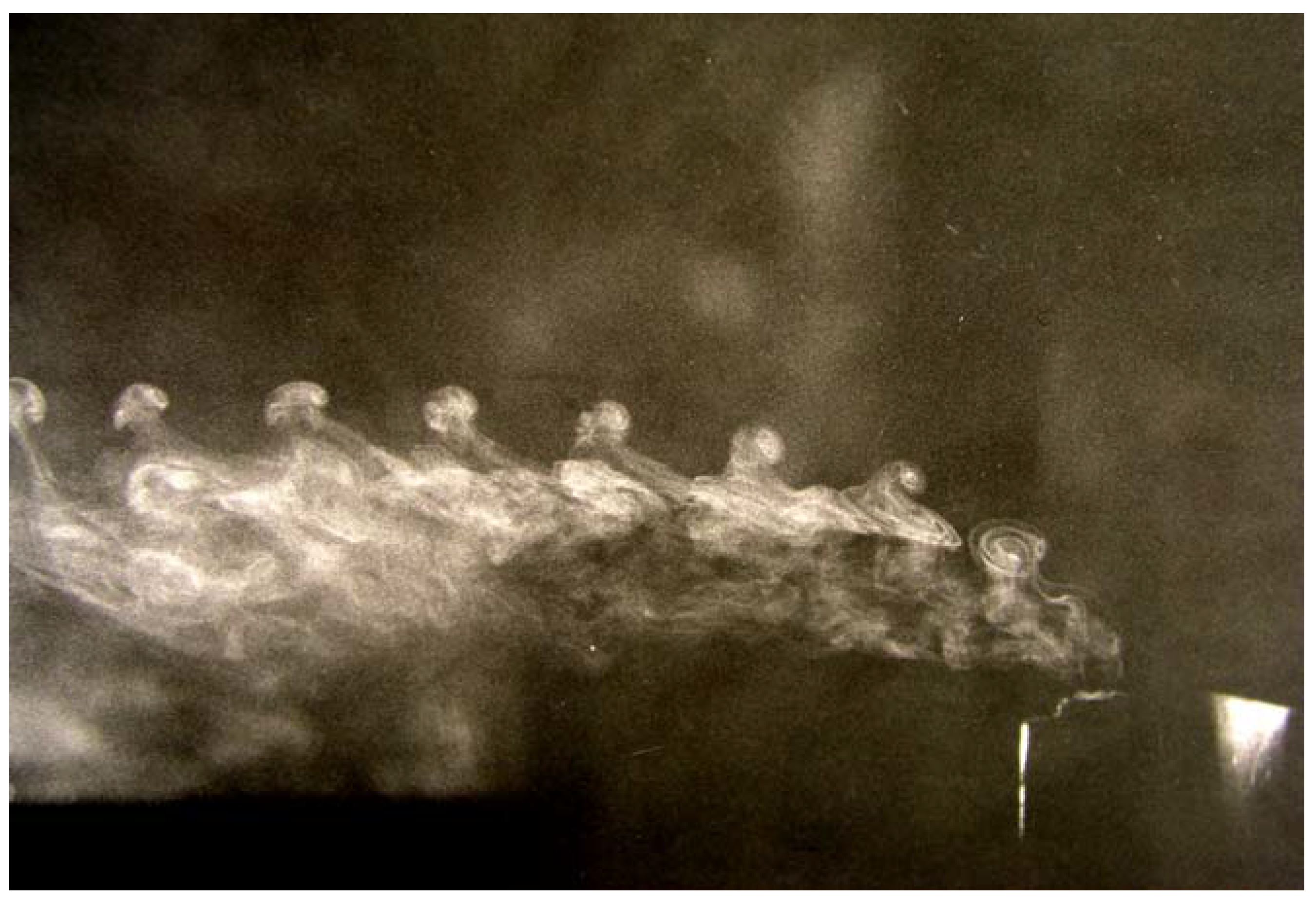
During a previous study of the behavior of an internal free shear layer within a flow cavity in a subsonic wind tunnel (Isaacson [
13]), a number of photographs of the flow structures along the shear layer were obtained. The flow conditions were not reported.
Figure 7 shows vertical flow structures in the physical domain that perhaps indicate an ordered value for the fluctuating vertical velocity. Note that
Figure 5 presents results obtained from the Fourier analysis of the shear layer equations that indicate a nearly constant fluctuating vertical velocity across a significant time frame of the integration.
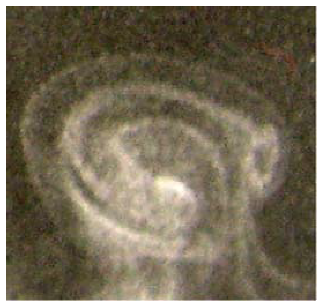
Figure 8 presents a close-up of the first flow structure shown in
Figure 7.
Figure 8 indicates a possible vortex tube-type structure, inclined to the vertical span-wise plane. Again, the Fourier analysis results presented in
Figure 6 indicate a periodic behavior for the
versus
phase plane. However, the physical flow structures shown in
Figure 7 and
Figure 8 cannot be deduced from the fluctuating wave results presented in
Figure 5 and
Figure 6.
Figure 7.
The flow is from right to left across the sharp edge lower baffle of an internal cavity. The flow conditions were not reported.
Figure 7.
The flow is from right to left across the sharp edge lower baffle of an internal cavity. The flow conditions were not reported.
Figure 8.
An expanded view of the forward structure shown in
Figure 7. The leftward slant of the structure may be due to the axial velocity of the mainstream flow.
Figure 8.
An expanded view of the forward structure shown in
Figure 7. The leftward slant of the structure may be due to the axial velocity of the mainstream flow.
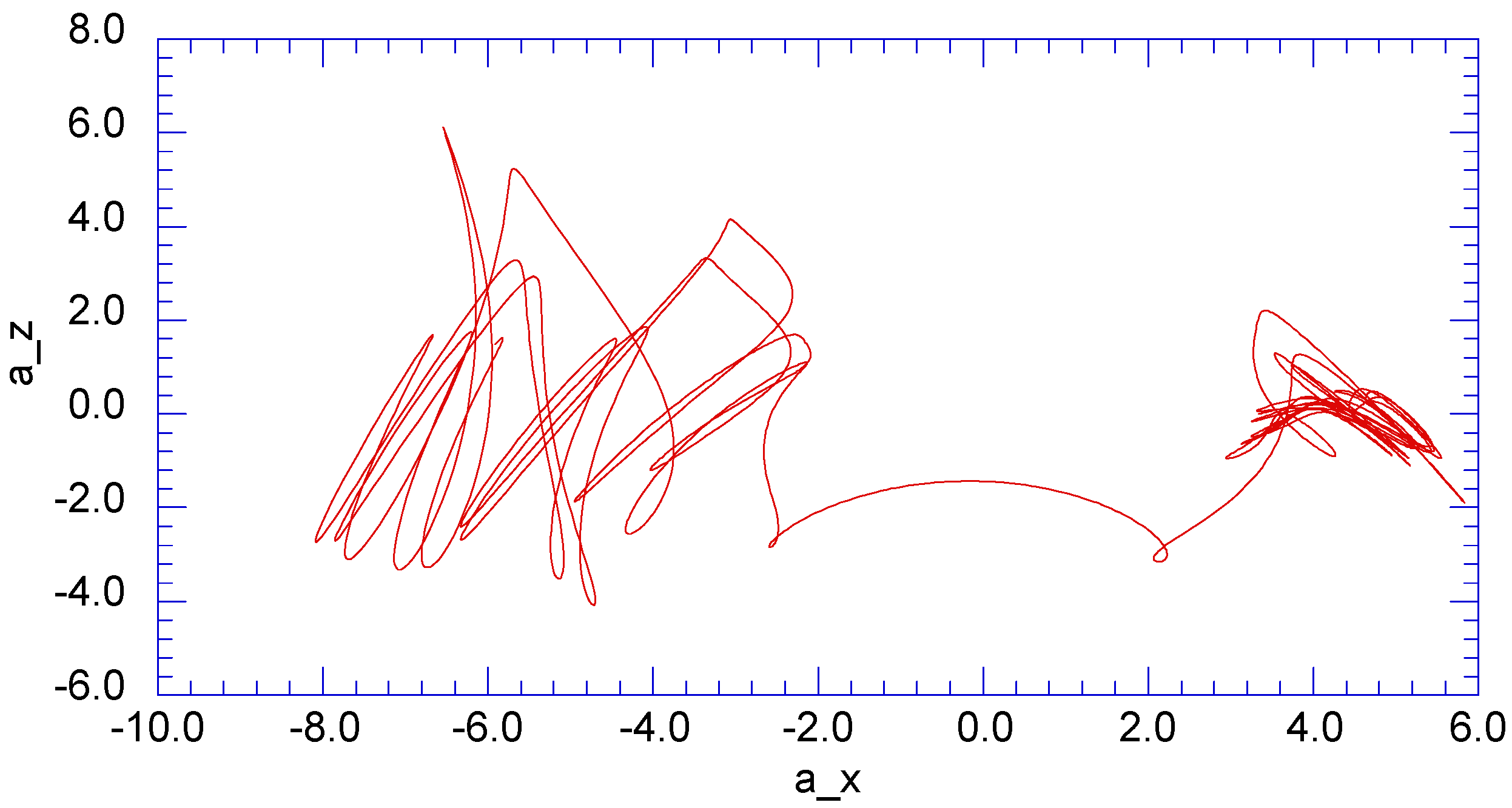
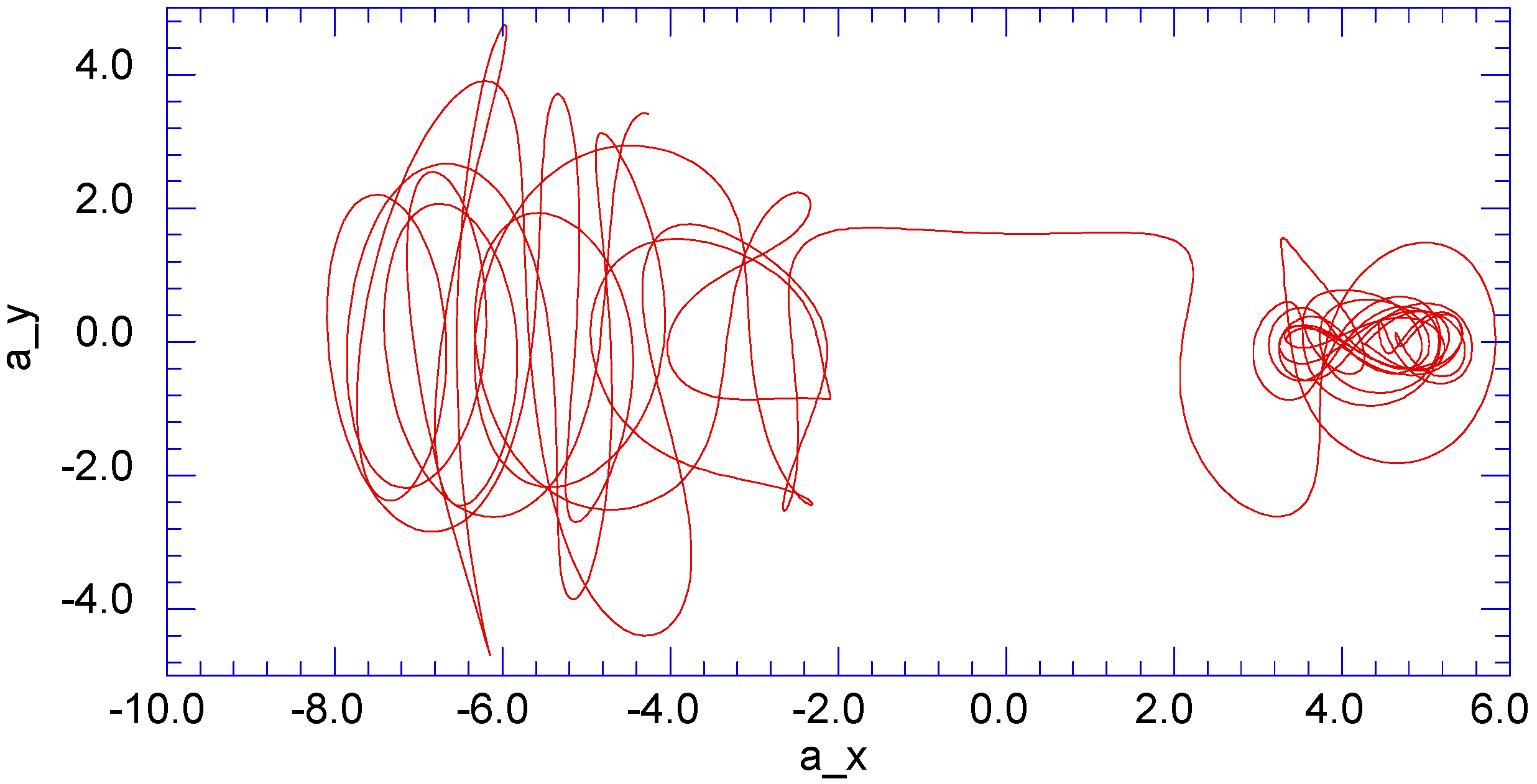
As the time step continues, the fluctuation in the axial velocity component reaches a negative value, causing a transition of the vertical velocity component to a significantly larger fluctuation in value (
Figure 9). It appears that as the fluctuating vertical and span-wise velocity components reach the region of increasing negative axial fluctuating velocity values, the system has reached a transition region, where the flow undergoes a significant change in behavior. Beyond this transition region, all three components of the flow velocity show large fluctuations in value (
Figure 10).
Figure 9.
The phase plane representation of the vertical velocity versus the horizontal velocity over 3,000 time steps for an area ratio
Figure 9.
The phase plane representation of the vertical velocity versus the horizontal velocity over 3,000 time steps for an area ratio
Figure 10.
The phase plane representation of the span-wise velocity versus the horizontal velocity over 3,000 time steps for an area ratio
Figure 10.
The phase plane representation of the span-wise velocity versus the horizontal velocity over 3,000 time steps for an area ratio
To obtain a numerical representation of this complex flow behavior, concepts from information theory as developed by Tribus [
32] are applied. From the basic formalism of information theory as developed by Jaynes [
7], Tribus expresses first the maximum of the entropy as described by the expression,
, where
represents the probability of finding the system in a given state
i. Second, a Lagrangian multiplier is applied to the reality condition,
. Finally, a second Lagrangian multiplier is applied to the conservation of overall energy of the system,
. Application of the formalism presented by Tribus [
32] leads to the distribution function for
in terms of a single Lagrangian multiplier,
, specified as the “temper” of the expected value of the energy of the system. The connection between the microscopic distribution function and the macroscopic concepts of thermodynamics is then made through an evaluation of the “pressure” of an ideal gas against the walls of the container of the system. Experimental comparison of the behavior of the “pressure” of the gas with the ideal gas equation yields the final result that
, where k is Boltzmann’s constant and T is the temperature of the system. More general considerations yield the result that thermal equilibrium between systems defines the equality of the “temperature” of the systems. The essential point is that recourse must be made to experimental observations to bring the concepts of information theory to agreement with macroscopic thermodynamics.
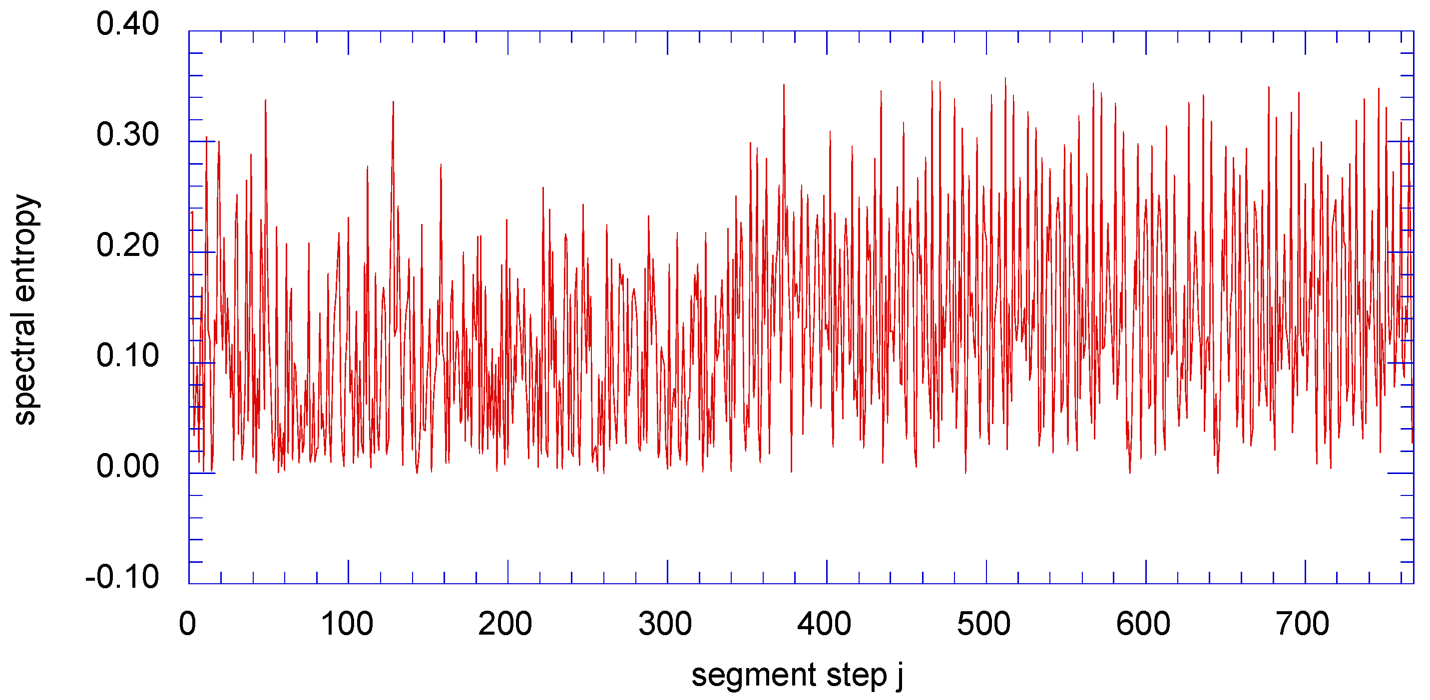
To establish a similar form for the set of equations describing the flow through a sudden expansion, we employed the following procedure: First, the physics of the internal shear layer were represented in the form of six first-order differential equations. The first three equations represent the conservation of mass through the system. Second, the integration of the equations of motion and the computation of the kinetic energy associated with the vertical and span-wise velocity fluctuations were computed. Third, local spectral entropy was computed for regions across the entire time span of the computation.
Figure 11 indicates that during the first of the time steps, the spectral entropy decreases, indicating an increase in information within the flow structures. The spectral entropy then increases over a relatively short time span as the flow transitions to the next region. In this region, the spectral entropy again decreases, again indicating an increase in the information content within the flow in that region. As the time steps continue, the flow transitions to the significant aperiodic behavior indicated in the remainder of
Figure 11.
This region of spectral entropy values contributes to the predicted spectral entropy of the overall flow into the sudden expansion. Note that these values of the spectral entropy occur when the fluctuating axial velocity is in the negative range and produces the most vigorous part of the aperiodic motion. Prichard and Theiler [
30] indicate that the most energetic of the fluctuating components of velocity will contribute to the spectral entropy through this region and that they will be subjected to the folding and stretching of the flow elements as they lose information to spectral entropy. This region is thus a region of “dissolution” where the incoming low spectral entropy flow is transformed into a high spectral entropy region. This region thus provides a flow reservoir of high spectral entropy elements which, through a “scrambling” process, reach the level of physical scales that ultimately dissipate into background thermodynamic entropy. Mathieu and Scott [
33] have discussed this “scrambling” process in much more detail. Sagaut and Camdon [
34] have described the flow of high spectral entropy elements into the dissipation region as a “streaming” process.
Figure 11.
Spectral entropy results for the fluctuating and velocity components by the maximum entropy method.
Figure 11.
Spectral entropy results for the fluctuating and velocity components by the maximum entropy method.
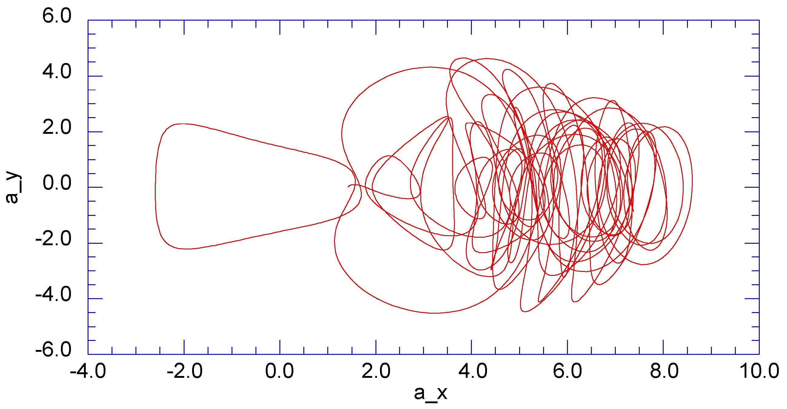
It is interesting to note that for the area ratios which produce the lowest inlet velocities, the results for the
versus phase plane indicate weak oscillations primarily in the positive
region. As the flow inlet velocity is increased, the flow oscillations in the positive
region become stronger. For an area ratio of
,
Figure 12 presents the phase plane representation of the vertical velocity component
versus the axial velocity component
for 3,000 time steps. The vertical fluctuations for this case also show a transition region toward the negative
region. However, these results indicate that the fluctuating vertical velocity component returns to the region of positive axial velocity fluctuations in a more orderly oscillation pattern.
Figure 12.
The phase plane representation of the fluctuating velocity component versus the fluctuating velocity component for a count of 3,000 time steps for an area ratio
Figure 12.
The phase plane representation of the fluctuating velocity component versus the fluctuating velocity component for a count of 3,000 time steps for an area ratio
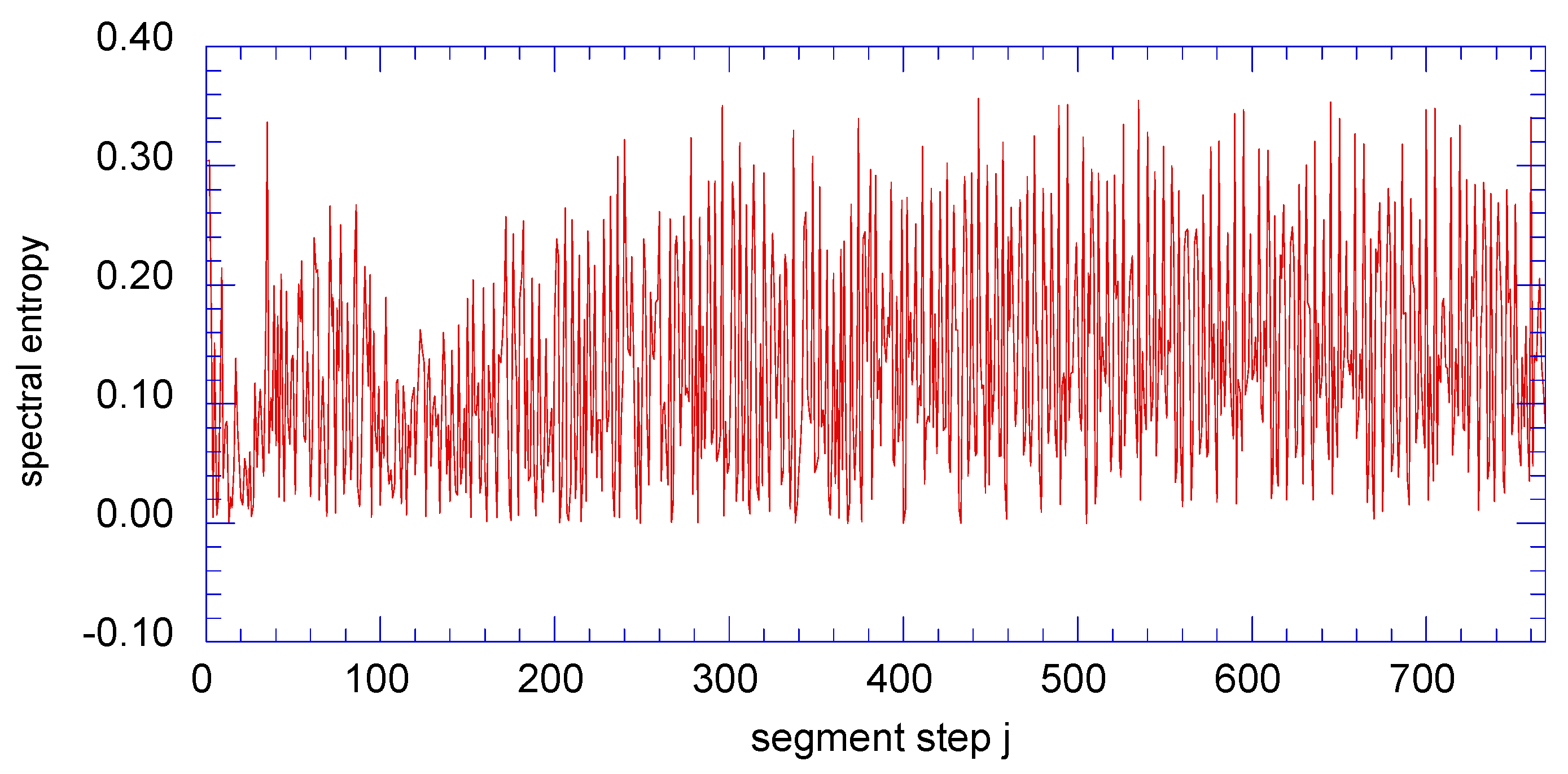
The spectral entropy results for the area ratio
are presented in
Figure 13 and cover the entire time step range. Although these results appear to be similar to the results presented in
Figure 11, it must be noted that the flow behavior is different. The initial fluctuating vertical velocities occur again in the positive fluctuating axial velocity range. Then, the fluctuating vertical velocities again transition toward the negative axial velocity region. However, instead of crossing into the negative axial velocity region, the fluctuating vertical velocity vectors return to the positive fluctuating axial velocity vector region. Hence, the results for the low inlet axial velocity indicate a different behavior with considerably reduced average spectral entropy content. These results imply the existence of a transition region in the flow as the inlet flow velocity is increased from the initial low values to the higher values.
Even though the maximum spectral entropy values for the case of area ratio
in
Figure 13 are similar to those for the area ratio of
, it becomes necessary to take a much lower value of the spectral entropy threshold, or activation spectral entropy, to provide a predicted value of spectral entropy increase to correspond with the experimentally inferred value.
Figure 13.
Spectral entropy results for the fluctuating and velocity components by the maximum entropy method for the area ratio
Figure 13.
Spectral entropy results for the fluctuating and velocity components by the maximum entropy method for the area ratio
As the inlet flow velocity is increased to an area ratio
, the oscillations of the
component in the negative fluctuating axial velocity region are quite pronounced, with a significant spectral entropy produced. Thus, the activation spectral entropy values are strong functions of the inlet axial flow kinetic energy. It should be noted that once the entropy increase across the flow region has been determined, all other thermodynamic parameters could be determined by the methods of classical gas dynamics (Saad [
35]).
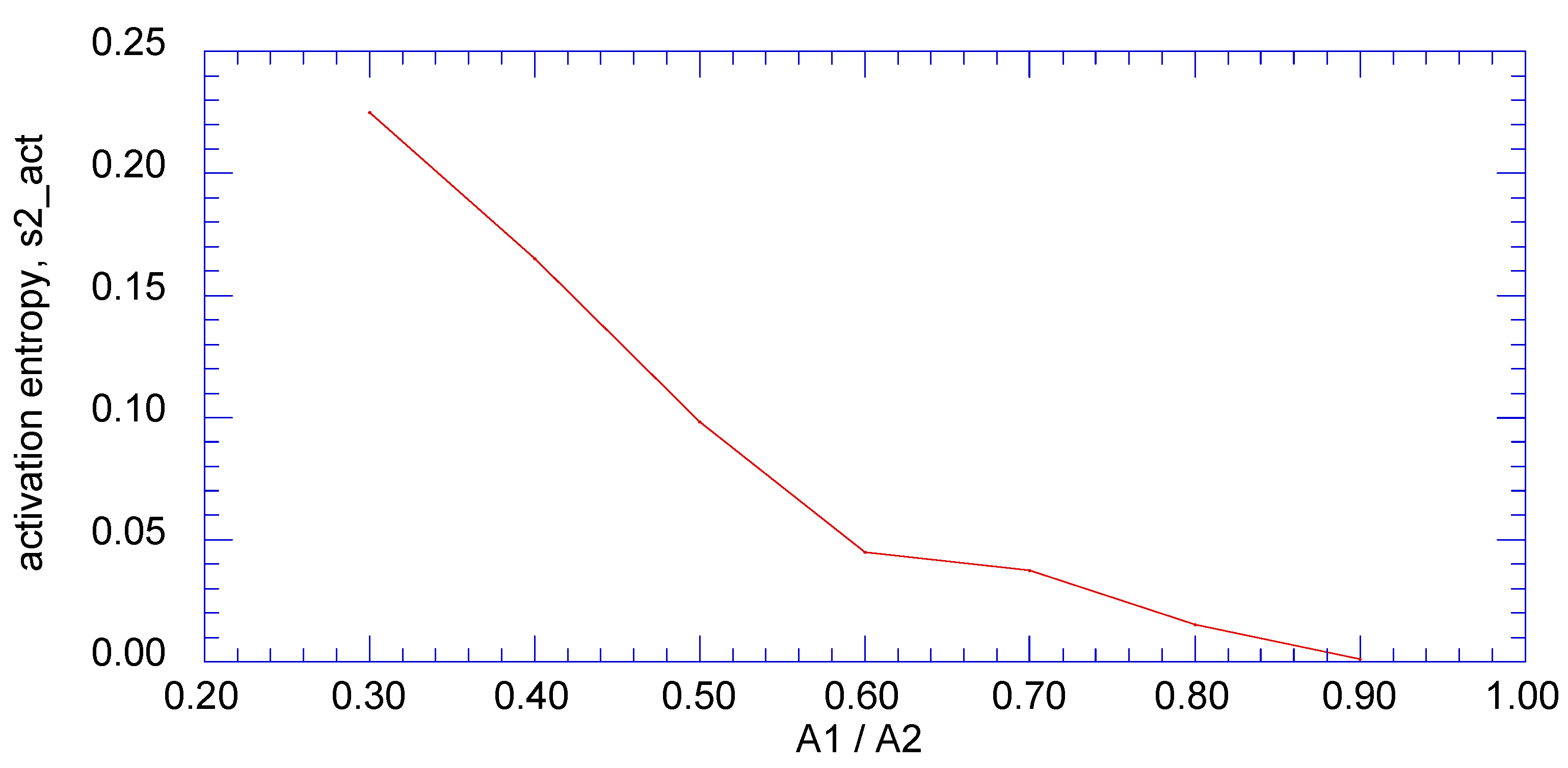
The computed spectral entropy value across the expansion for each applied area ratio required the introduction of the threshold spectral entropy value. All of the spectral entropy values above the threshold were then averaged over the time step range to get the computed value to come into agreement with the inferred experimental entropy. The corresponding threshold spectral entropy values, or activation spectral entropies, are shown in
Figure 14. The introduction of the activation spectral entropy above which the average of the spectral entropy values come into agreement with the experimentally-inferred values of overall entropy increase implies the existence of a potential barrier for the production of spectral entropy components which contribute to the overall irreversibility of the expansion process. Thus, thus, those more disordered structures which cross this threshold provide a reservoir of such disordered structures, which then decay into structures of the scale that dissipate into background thermodynamic entropy.
Figure 14.
Values of the activation spectral entropy as a function of the area ratio,
Figure 14.
Values of the activation spectral entropy as a function of the area ratio,
With the inclusion of the activation spectral entropy in the computations for the spectral entropy values across the range of expansion area ratios, the results for the computed spectral entropy values are brought into agreement with the implied measured entropy values.
4. Experimental Values for the Increase of Entropy
The experimental results for the loss of stagnation pressure across a dump combustor as measured by Barclay [
8], and as correlated by Oates [
9] serve as the benchmark against which we compare our theoretical predictions. The flow configurations that were used in the experimental project were circular ducts of different area ratios with abrupt expansions. The flow consisted of air and the flow was subsonic throughout. The inferred entropy changes across the expansion were obtained from the experimental results through the following analysis.
The Gibbs equation of thermodynamics may be written, in terms of stagnation properties, as:
In this equation,
is the stagnation temperature,
s is the entropy,
is the stagnation enthalpy,
is the stagnation specific volume, and
is the stagnation pressure. For the adiabatic flow of an ideal gas, this may be integrated to the following expression, with R as the appropriate gas constant:
Hence, given the experimental value for the decrease in stagnation pressure across the expansion, we may evaluate the experimental increase of entropy as:
This expression yields the dimensionless change in entropy for a given change in stagnation pressure from thermodynamic state 1 to thermodynamic state 2.
The series of experiments conducted by Barclay [
8] yielded values for the loss in stagnation pressure across a “dump” combustor. The flow geometry consisted of a circular pipe of area
with a sudden expansion into a downstream circular pipe of area
, with the experiments conducted for a range of area ratios from
Oates [
9] reports that the experimental results may be expressed as:
In this equation,
is the ratio of specific heats and
is the Mach number of the flow at area
. This expression is used to obtain the dimensionless entropy increase across the sudden expansion for the range of area ratios
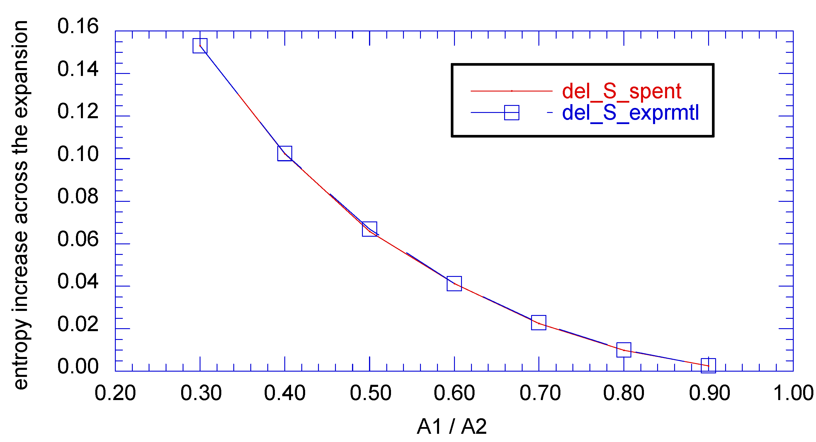
. These results then serve as the test base against which the theoretical calculations are compared. The comparisons of the results are presented in
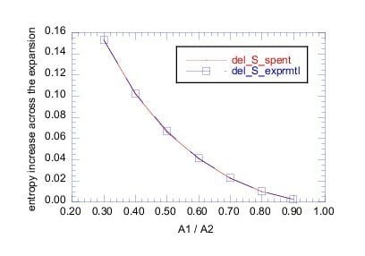
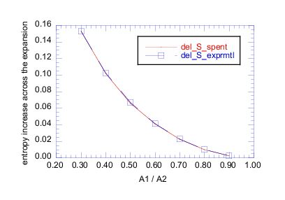
Figure 15 and represent the overall results for this study.
Figure 15.
Comparison of the computed spectral entropy increase with the experimental increase in entropy obtained from the measured loss of stagnation pressure as a function of the area ratio .
Figure 15.
Comparison of the computed spectral entropy increase with the experimental increase in entropy obtained from the measured loss of stagnation pressure as a function of the area ratio .
The introduction of the threshold spectral entropy, which we have called the activation spectral entropy is the ad hoc connection of the deterministic numerical predictions of the spectral entropy content with the experimentally inferred increase in entropy across the sudden expansion. We anticipate that future developments will provide a rational connection between the deterministic numerical results and the actual irreversible processes that occur in physical systems.
Table 1 presents the computed results for the increase of spectral entropy for each of the area ratios in the expansion process together with the inferred increase in entropy for the corresponding experimental area ratios. In
Table 1,
is the ratio of the inlet area to the exit area,
is the overall average of the spectral entropy series,
is the activation spectral entropy,
is the spectral entropy average above the activation spectral entropy,
_spent is the predicted spectral entropy increase, and
_exprmtl is the experimentally inferred value of the entropy increase.
Table 1.
Summary of predicted entropy increases and corresponding experimentally inferred entropy values for the flow through a sudden expansion.
Table 1.
Summary of predicted entropy increases and corresponding experimentally inferred entropy values for the flow through a sudden expansion.
| A1/A2 | s1_spent | s2_act | s2_spent | ΔS_spent | ΔS_exprmtl |
|---|
| 0.30 | 0.1271 | 0.2250 | 0.2802 | 0.1531 | 0.1531 |
| 0.40 | 0.1097 | 0.1650 | 0.2119 | 0.1022 | 0.1025 |
| 0.50 | 0.1255 | 0.0983 | 0.1913 | 0.0658 | 0.0669 |
| 0.60 | 0.0748 | 0.0450 | 0.1161 | 0.0413 | 0.0414 |
| 0.70 | 0.1303 | 0.0375 | 0.1529 | 0.0226 | 0.0229 |
| 0.80 | 0.0929 | 0.0153 | 0.1029 | 0.0100 | 0.0101 |
| 0.90 | 0.1232 | 0.0012 | 0.1258 | 0.0026 | 0.0025 |


