Increasing and Decreasing Returns and Losses in Mutual Information Feature Subset Selection

Abstract

Mutual information between a target variable and a feature subset is extensively used as a feature subset selection criterion. This work contributes to a more thorough understanding of the evolution of the mutual information as a function of the number of features selected. We describe decreasing returns and increasing returns behavior in sequential forward search and increasing losses and decreasing losses behavior in sequential backward search. We derive conditions under which the decreasing returns and the increasing losses behavior hold and prove the occurrence of this behavior in some Bayesian networks. The decreasing returns behavior implies that the mutual information is concave as a function of the number of features selected, whereas the increasing returns behavior implies this function is convex. The increasing returns and decreasing losses behavior are proven to occur in an XOR hypercube.

1. Introduction

Feature subset selection [1] is an important step in the design of pattern recognition systems. It has several advantages. First, after feature selection has been performed off-line, predictions of a target variable can be made faster on-line, because predictions can be performed in a lower-dimensional space and only a subset of the features needs to be computed. Secondly, it can lead to a decrease in hardware costs, because smaller patterns need to be stored or sensors that do not contribute to the prediction of a target variable can be eliminated (see e.g. [2] for a recent application of sensor elimination by means of feature subset selection). Thirdly, it can increase our understanding of the underlying processes that generated the data. Lastly, due to the curse of dimensionality [1,3], more accurate predictions can often be obtained when using the reduced feature set. Depending on the context, ‘feature selection’ is sometimes called ‘characteristic selection’ [4] or ‘variable selection’ [5].

Mutual information between the target variable, denoted as ‘C’, and a set of features, denoted as {F${}_1$,…F${}_n$}, is a well-established criterion to guide the search for informative features. However, some pitfalls in mutual information based feature subset selection should be avoided. A well-known property of entropy, i.e., conditioning reduces uncertainty, does not necessarily hold for the mutual information criterion in feature selection. It would imply that conditioning on more features reduces the information that a feature contains about the target variable. Conditioning reduces information has been assumed to hold sometimes in the approximation of the high-dimensional mutual information by means of lower-dimensional mutual information estimations [6,7]. However, we show in this paper, using some counterexamples, related to the bit parity problem, that conditioning can increase the mutual information of a feature or a feature set about a target variable. We show in Section 3 that this can hold for both discrete, either binary or non-binary, and continuous features. Most lower-dimensional mutual information estimators may perform weak when dealing with probability distributions in which conditioning can increase information, see Section 4.4.

It has been observed sometimes that increments in mutual information become smaller and smaller in a sequential forward search in [8]. In fact, in this paper, we prove by means of a counterexample that the opposite behavior can also occur: the increments in mutual information become larger and larger in the SFS. This increasing returns behavior could be proven to occur in a (2n+1)-(2n-1)-…5-3 XOR hypercube in Section 4.1. The decreasing returns behavior, i.e., increments in mutual information become smaller and smaller, could be proven to occur in some Bayesian networks in Section 4.2. We show in Section 5.1 that the ‘increasing returns’ has a comparable ‘decreasing losses’ implication in the sequential backward search. In Section 5.2, we show that the ‘decreasing returns’ has a comparable ‘increasing losses’ implication in the sequential backward search. All our theoretical claims are supported and illustrated by experiments.

2. Background and Definitions

2.1. Historical Background

Lewis was among the first to apply mutual information as a feature selection criterion almost half a century ago [4]. Mutual information was used to select good characteristics in a letters and numerals prediction problem. The following years the criterion was applied by Kamentsky and Liu in [9] and Liu in [10] to similar character recognition problems. Although at that time Lewis did not call his criterion ‘mutual information’, but a ‘measure of goodness’ G${}_i$:

$$G_i=\sum _{f_i,c}p(f_i,c)log\left(\frac{p(f_i|c)}{p(f_i)}\right)$$

(1)

Multiplying both the numerator and the denominator within the logarithm with p(c), this leads to the mutual information criterion for feature selection, used extensively since [11]:

$$MI(F_i;C)=\sum _{f_i,c}p(f_i,c)log\left(\frac{p(f_i,c)}{p(f_i).p(c)}\right)$$

(2)

This expression for mutual information is also the one used in [12]. For a subset of features F${}_S$ = {F${}_{S1}$,F${}_{S2}$, … F${}_{Sn1}$}, this is:

$$MI({\mathit{F}}_S;C)=\sum _{{\mathit{f}}_s,c}p({\mathit{f}}_s,c)log\left(\frac{p({\mathit{f}}_s,c)}{p({\mathit{f}}_s).p(c)}\right)$$

(3)

The mutual information can be expanded in entropy terms H(C) and H(C∣F${}_S$) as:

$$MI({\mathit{F}}_S;C)=H(C)-H(C|{\mathit{F}}_S)$$

(4)

Throughout the article, we use bold style to denote vectors, capitals to denote variables and lowercase letters to denote values of variables.

2.2. Conditional Mutual Information

The conditional mutual information of feature F${}_i$ and C, given F${}_j$, is defined as [12]:

$$MI(F_i;C|F_j)=\sum _{f_i,f_j,c}p(f_i,f_j,c)log\left(\frac{p(f_i,c|f_j)}{p(f_i|f_j).p(c|f_j)}\right)$$

(5)

Due to the chain rule for information [12], the conditional mutual information is equal to a difference in (unconditional) mutual information:

$$MI(F_i;C|F_j)=MI(F_i,F_j;C)-MI(F_j;C)$$

(6)

3. Conditioning Increases Information

One particular example where conditioning on additional variables can increase information was given in [12] (see page 35). The example was Z = X + Y, with X and Y binary independent distributed variables. Then, it was shown that MI(X;Y) < MI(X;Y∣Z). We provide examples in this section that are more tailored to the feature subset selection problem, and also show that it holds for binary, non-binary discrete and continuous features. The n-bit parity problem and the checkerboard pattern were also mentioned in [5] to indicate that a variable which is useless by itself can be useful together with others. We derive the implications for these examples for conditioning in mutual information based feature selection. We provide results for ‘n’ features in general and derive a general ‘conditioning increases information’ result in inequality (11) under the conditions given in (7) and (9).

3.1. n-bit Parity Problem

The bit parity problem is frequently used as a benchmark problem, e.g. in neural network learning [13]. Consider ‘n’ independent features F${}_1$,… F${}_n$ that are binary: F${}_i$∈ {0,1} and p(F${}_1$,F${}_2$, …F${}_n$) = ${\prod }_{i=1}^n$ p(F${}_i$).

The target variable in the case of the n-bit parity problem, which is an XOR problem for n = 2, is then defined as:

$$C=mod(\sum _{i=1}^n{F}_i,2)$$

(7)

We denote the modulo 2 computation by mod(.,2). The target variable is equal to 1 in case the n-tuple (f${}_1$,f${}_2$, …f${}_n$) contains an odd number of 1’s and is 0 otherwise. The mutual information based on the full feature set is equal to:

$$\begin{array}{cc}MI(F_1,F_2,\dots F_n;C)& =H(C)-H(C|F_1,F_2,\dots F_n)\hfill \\ & =H(C)\hfill \end{array}$$

(8)

where Equation (8) is due to the result that the uncertainty left about C after observing F${}_1$, F${}_2$, …F${}_n$ is equal to 0: H(C∣F${}_1$,F${}_2$, …F${}_n$) = 0. The probability of class 0, p(c=0), and class 1, p(c=1), is equal to 1/2 for n ≥ 2, this implies that according to Equation (8) the mutual information MI(F${}_1$,F${}_2$,…F${}_n$;C) = 1 bit. In the previous computation, we used the base 2 logarithm. In case the target variable takes 2 values, C ∈ {0,1}, the mutual information will be maximally 1 bit, in fact, in (3) one can choose the base of the logarithm. For any strict subset F${}_S$⊂{F${}_1$,F${}_2$,…F${}_n$} excluding $\varnothing$, it can be verified that p(f${}_S$,c) = p(f${}_S$).p(c). From this, it follows that, using the definition of mutual information in Equation (3), MI(F${}_S$;C) = 0. This leads us to the following result. Suppose that:

$$\begin{array}{ccc}\hfill \{F_1,F_2,\dots F_n\}& =& {\mathit{F}}_{S1}\cup {\mathit{F}}_{S2},\hfill \\ \hfill \mathrm{with}{\mathit{F}}_{S1}\ne \varnothing ,{\mathit{F}}_{S2}\ne \varnothing & \mathrm{and}& {\mathit{F}}_{S1}\cap {\mathit{F}}_{S2}=\varnothing \hfill \end{array}$$

(9)

Because F${}_{S1}$ and F${}_{S2}$ are strict subsets of the full feature set, it holds that MI(F${}_{S1}$;C) = 0 and MI(F${}_{S2}$;C) = 0 in the n-dimensional XOR problem. For the conditional mutual information, it holds that:

$$\begin{array}{ccc}\hfill MI({\mathit{F}}_{S2};C|{\mathit{F}}_{S1})& =& MI({\mathit{F}}_{S1},{\mathit{F}}_{S2};C)-MI({\mathit{F}}_{S1};C)\hfill \\ & =& 1-0\hfill \end{array}$$

(10)

From this, we can derive following general result:

$$\begin{array}{c}\hfill MI({\mathit{F}}_{S2};C|{\mathit{F}}_{S1})>MI({\mathit{F}}_{S2};C)\end{array}$$

(11)

Similarly, we can conclude: MI(F${}_{S1}$;C∣F${}_{S2}$) > MI( F${}_{S1}$;C).

A case derived from the n-bit parity problem is obtained when the variable F${}_j$ and C are interchanged in Equation (7):

$$F_j=mod(\sum _{i=1,i\ne j}^n{F}_i+C,2)$$

(12)

with all the variables F${}_{i,i\ne j}$ and C independent and binary. For this case it holds that MI(F${}_1$,…F${}_{j-1}$,F${}_{j+1}$,…F${}_n$;C) = 0, because {F${}_1$,…F${}_{j-1}$, F${}_{j+1}$,…F${}_n$} and C are independent by construction. However, after conditioning on F${}_j$ we obtain:

$$\begin{array}{ccc}\hfill MI(F_1,\dots F_{j-1},F_{j+1},\dots F_n;C|F_j)& =& H(C|F_j)-H(C|F_1,F_2,\dots F_n)\hfill \end{array}$$

(13)

$$\begin{array}{ccc}& =& H(C|F_j)=1\hfill \end{array}$$

(14)

In Equation (13) H(C∣F${}_1$,F${}_2$,…F${}_n$) = 0, because after all other features are observed, C can be perfectly predicted. In Equation (14) H(C∣F${}_j$) = H(C), because F${}_j$ on its own contains no information about C. Hence, for Equation (12) we conclude: MI(F${}_1$,…F${}_{j-1}$,F${}_{j+1}$,…F${}_n$;C∣F${}_j$) > MI(F${}_1$,…F${}_{j-1}$,F${}_{j+1}$,…F${}_n$;C). In fact, for Equation (12), the more general result of inequality (11) also holds under the conditions of (9), regardless whether F${}_j$ ∈ F${}_{S1}$ or F${}_j$ ∈ F${}_{S2}$.

3.2. Non-binary Discrete Features

Consider the checkerboard pattern shown in Figure 1.

Figure 1. Checkerboard pattern.

Figure 1. Checkerboard pattern.

The target variable C is noted in the squares and depends on whether the square is black (c = 0) or white (c = 1). There are two features F${}_1$ and F${}_2$, corresponding to the column and row indicators, respectively. Variables F${}_1$ and F${}_2$ are 8-ary and take values {1,2,3,…8}, while C is binary. How does this checkerboard pattern relate to the n-bit parity problem? The pattern in Figure 1 can be seen as a natural extension of the n-bit parity problem and can also be expressed by Equation (7) with the same requirement of independence between features. In the case of m-ary features, with ‘m’ even, it holds that any strict subset of features contains no information about the target variable. The requirement of ‘m’ even arises from the fact that, for any subset of features, we need an equal number of 0 and 1 cells in order for strict subsets not to be informative, this can only be achieved when ‘m’ is even (see also Section 4). The full feature set for ‘m’ even contains 1 bit of information. This shows that the general result of inequality (11) also holds for non-binary discrete features.

A concept related to mutual information is the n-way interaction information introduced by McGill [14]. This n-way interaction information has been used to characterize statistical systems such as spin glasses in [15], where the concept was introduced as ‘higher-order mutual information’. The n-way interaction information for class variable C and features F${}_1$, F${}_2$,…F${}_n$, written as I${}_{n+1}$(C,F${}_1$,F${}_2$,…F${}_n$), can be expressed in terms of the mutual information as follows:

$$\begin{array}{c}\hfill I_{n+1}(C,F_1,F_2,\dots F_n)=\sum _{k=1}^n{(-1)}^{(k+1)}\sum _{i_1<\dots <i_k}MI(F_{i_1},F_{i_2},\dots F_{i_k};C),\end{array}$$

(15)

with {i${}_1$, i${}_2$,…i${}_k$} ∈ {1,2,…n}. As opposed to the usual mutual information, the higher-order mutual information can be negative. The statistical system is termed ‘frustrated’ in that case [15]. The XOR problem presented in Figure 1 is an example of a frustrated system, because I${}_{n+1}$(C,F${}_1$,F${}_2$,…F${}_n$) = -MI(F${}_1$,F${}_2$;C)=-H(C). However, it is observed that the XOR problem appears as ‘frustrated’ if the number of features is even. In case of an odd number of features, the higher-order mutual information is positive, e.g. for n = 3 features I${}_{n+1}$(C,F${}_1$,F${}_2$,…F${}_n$) = MI(F${}_1$,F${}_2$,F${}_3$;C) = H(C). The n-way interaction information can be useful in feature selection to verify whether any of the features is independent of all other features and the target variable in a single test. This can be seen from Equation (15): the n-way interaction information is symmetric (see [14]), one can exchange the class variable with any feature. Hence, if for any F${}_j$ MI(F${}_1$,…F${}_{j-1}$,F${}_{j+1}$,…F${}_n$,C;F${}_j$) = 0, then I${}_{n+1}$(C,F${}_1$,F${}_2$,…F${}_n$) = 0. Three-way interaction information has been used to derive causal relationships between neurons in [16] and more recently between features and the target variable in [17].

All examples above were given for discrete features, the question is whether the ‘conditioning increases information’ result can also hold for continuous features.

3.3. Continuous Features: Mixture Models

Consider a d-dimensional Gaussian mixture model (GMM) or t mixture model (tMM), with the number of Gaussians or t distributions equal to 2${}^d$, with half of the Gaussians or t distributions assigned to class 0, and the other half to class 1, and where each distribution has a mixing proportion of 1/(2${}^d$). An example is provided in Figure 2, where the Gaussians are positioned on a cube with corners (${\mu }_1$, ${\mu }_2$, ${\mu }_3$) ∈{(0,0,0), (1,0,0),…(1,1,1)}, the covariance matrices are spherical and d = 3.

Figure 2. Gaussian distributions with spherical covariance matrices on cube corners.

Figure 2. Gaussian distributions with spherical covariance matrices on cube corners.

Suppose that we assign the Gaussians for which mod(${\mu }_1$ + ${\mu }_2$ + ${\mu }_3$,2) = 1 to class 1 (light grey in Figure 2) and the Gaussians for which mod(${\mu }_1$ + ${\mu }_2$ + ${\mu }_3$,2) = 0 to class 0. (dark grey). This Gaussian mixture model can be written as:

$$\begin{array}{c}\hfill \sum _{\begin{array}{c}i=1:2^{(3-1)},\\ mod({\mu }_{i1}+{\mu }_{i2}+{\mu }_{i3},2)=0\end{array}}\frac{1}{2^3}\mathcal{N}(\left[\begin{array}{c}{\mu }_{i1}\\ {\mu }_{i2}\\ {\mu }_{i3}\end{array}\right],\Sigma )+\end{array}$$

$$\begin{array}{c}\hfill \sum _{\begin{array}{c}j=2^{(3-1)}+1:2^{(3)},\\ mod({\mu }_{j1}+{\mu }_{j2}+{\mu }_{j3},2)=1\end{array}}\frac{1}{2^3}\mathcal{N}(\left[\begin{array}{c}{\mu }_{j1}\\ {\mu }_{j2}\\ {\mu }_{j3}\end{array}\right],\Sigma )\end{array}$$

(16)

The marginal distributions of a multivariate Gaussian distribution or multivariate t distribution are Gaussian and t distributed again [18], respectively. Hence, when we select 2 features, the marginal distributions are Gaussian again, and their centers will now be located on the corners of the square (0,0), (0,1), (1,0), (1,1). Moreover, on each corner, there will be 1 Gaussian from both classes, and in the case of equal covariance matrices, their distributions will be equal. Equal distributions for both classes implies that the mutual information with the target variable is equal to 0. This can be seen from the continuous version of mutual information:

$$\begin{array}{c}\hfill MI(F_1,F_2,\dots F_d;C)=\sum _c\underset{f_1,f_2,\dots f_d}{\int \int \int }p(f_1,f_2,\dots f_d,c)log\frac{p(f_1,f_2,\dots f_d,c)}{p(f_1,f_2,\dots f_d).p(c)}d{f}_{1}d{f}_2\dots d{f}_d\end{array}$$

(17)

The numerator in Equation (17), after subset selection with $sn1$ features, with $sn1$ < d and $sn1$ > 0, is equal to p(f${}_{s1}$,…f${}_{sn1}$,c), and the denominator is equal to:

$$\begin{array}{ccc}\hfill p(f_{s1},\dots f_{sn1}).p(c)& =& (p(f_{s1},\dots f_{sn1}|c=0).p(c=0)\hfill \\ & +& p(f_{s1},\dots f_{sn1}|c=1).p(c=1)).p(c)\hfill \\ & =& p(f_{s1},\dots f_{sn1},c)\hfill \end{array}$$

(18)

In Equation (18), we have that p(f${}_{s1}$,…f${}_{sn1}$∣c=0) = p(f${}_{s1}$,…f${}_{sn1}$ ∣c=1) = p(f${}_{s1}$,…f${}_{sn1}$∣c). Hence, the numerator and the denominator are equal in the MI definition and MI(F${}_1$,…F${}_{sn1}$;C) = 0 holds. This can be extended to more than 3 dimensions. Again the general result of inequality (11) applies. It is important to note that we only require the covariance matrices for the Gaussian distributions to be equal, not necessarily spherical, and in the case of multivariate t distributions, one additionally requires their degrees of freedom to be equal to guarantee that MI(F${}_1$,…F${}_{sn1}$;C) = 0.

4. Increasing and Decreasing Returns

4.1. Increasing Returns

Previously, it was found in [8] that in the sequential forward search (SFS), when features are selected later in the forward search, they contribute less in the increase of information of the target variable compared to previously selected ones. Let us illustrate this with an example. Suppose that we dispose of 3 features F${}_1$, F${}_2$ and F${}_3$ and that F${}_1$ is the first feature for which MI(F${}_1$;C) > MI(F${}_2$;C) > MI(F${}_3$;C). In the first iteration of the SFS, the feature, for which the objective MI(F${}_i$;C) is the highest, is selected. In this case, the selected feature will be F${}_1$. Suppose that in the second iteration of the SFS, we have: MI(F${}_2$;C∣F${}_1$) > MI(F${}_3$;C∣F${}_1$). The second selected feature will be F${}_2$. In the third iteration, the only feature left is F${}_3$ and the incremental increase in information is: MI(F${}_3$;C∣F${}_1$,F${}_2$). The ‘decreasing returns’ (i.e. every additional investment in a feature results in a smaller return) is then observed as: MI(F${}_1$;C) > MI(F${}_2$;C∣F${}_1$) > MI(F${}_3$;C∣F${}_1$,F${}_2$). However, this is not always true. 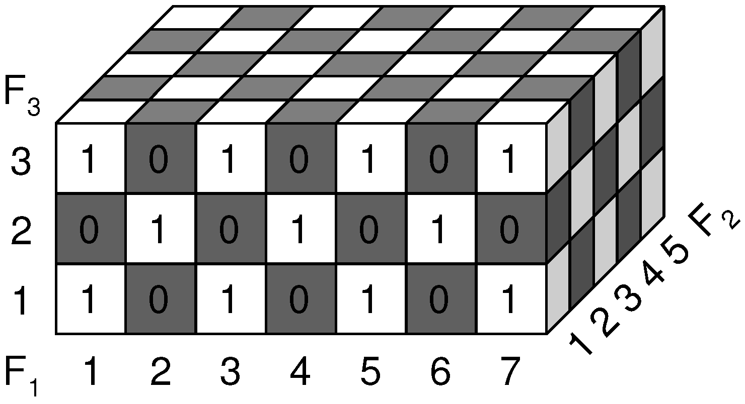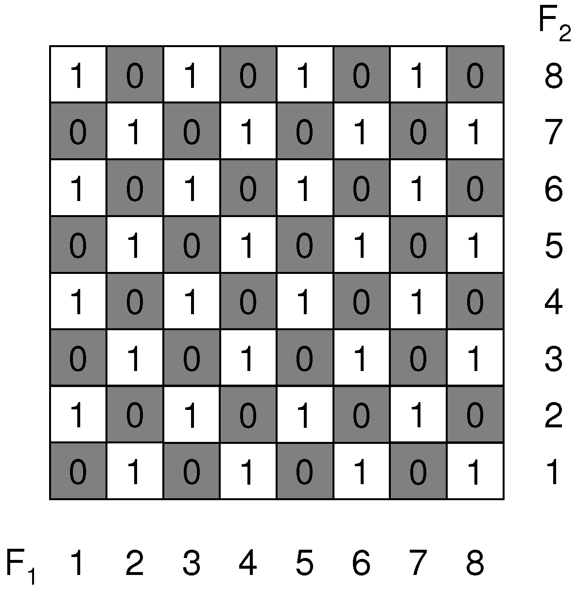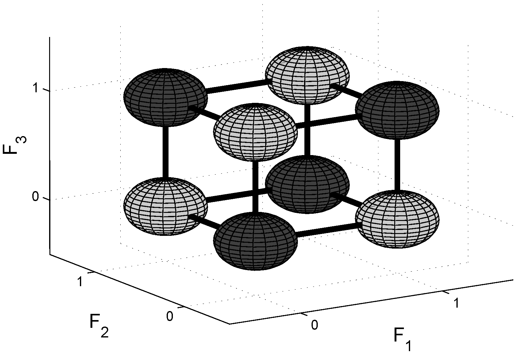We show with a counterexample that the opposite behavior can occur: although the order of selected features is F${}_1$, F${}_2$ and finally F${}_3$, it can hold that MI(F${}_1$;C) < MI(F${}_2$;C∣F${}_1$) < MI(F${}_3$;C∣F${}_1$,F${}_2$), i.e. we observe ‘increasing returns’ (every additional investment in a feature results in an increased return) instead of decreasing returns. Consider a possible extension of the checkerboard to 3 dimensions in Figure 3.

Figure 3. 7-5-3 XOR Cube. Extension of checkerboard to 3 dimensions, the number of values that each feature can take is odd and different for each feature.

Figure 3. 7-5-3 XOR Cube. Extension of checkerboard to 3 dimensions, the number of values that each feature can take is odd and different for each feature.

Here, the three features F${}_1$, F${}_2$ and F${}_3$ take an odd number of values: 7, 5 and 3 respectively. We will refer to this example as ‘7-5-3 XOR’. As opposed to ‘m’ even, now each feature individually, as well as each subset of features, contains information about the target variable. We computed the conditional entropies for this example in Table 1.

The mutual information and the conditional mutual information can be derived from the conditional entropies and are shown on the right side of the table. Clearly, the first feature that will be selected is F${}_1$, as this feature contains individually the most information about the target variable. The next feature selected is F${}_2$, because conditioned on F${}_1$, F${}_2$ contains the most information. Finally, F${}_3$ will be selected with a large increase in information: MI(F${}_3$;C∣F${}_1$,F${}_2$) ≈ 0,9183 bits. This increasing returns behavior can be shown to hold more generally for a $(2n+1)-\dots -7-5-3$ XOR hypercube, with ‘n’ the number of features. The total number of cells (feature value combinations) in such a hypercube is equal to $(2n+1).(2n-1).(2n-3)\dots (3)$. This can be written as a double factorial:

$$(2n+1)!!=(2n+1).(2n-1).(2n-3)\dots 3$$

(19)

This is an odd number of cells. $((2n+1)!!-1)/2$ of the cells have been assigned a 0 or a 1 value. The entropy H(C) can therefore be written as:

$$\begin{array}{c}\hfill H(C)=-\frac{(2n+1)!!-1}{2.(2n+1)!!}log\left(\frac{(2n+1)!!-1}{2.(2n+1)!!}\right)\\ \hfill -\frac{(2n+1)!!+1}{2.(2n+1)!!}log\left(\frac{(2n+1)!!+1}{2.(2n+1)!!}\right)\end{array}$$

(20)

Table 1. 7-5-3 XOR Cube. Entropies and Mutual Information for the SFS, NA = not available.

Entropy	value(bit)	Mutual Inf.	value(bit)
H(C)	-$\frac{53}{105}$log${}_2$ $\frac{53}{105}$ -$\frac{52}{105}$log${}_2$ $\frac{52}{105}$ ≈ 0,9999	NA	NA
H(C∣F${}_1$)	-$\frac{8}{15}$log${}_2$ $\frac{8}{15}$ -$\frac{7}{15}$log${}_2$ $\frac{7}{15}$ ≈ 0,9968	MI(F${}_1$;C)	≈ 3,143.10${}^{-3}$
H(C∣F${}_2$)	-$\frac{10}{21}$log${}_2$ $\frac{10}{21}$ -$\frac{11}{21}$log${}_2$ $\frac{11}{21}$ ≈ 0,9984	MI(F${}_2$;C)	≈ 1,571.10${}^{-3}$
H(C∣F${}_3$)	-$\frac{18}{35}$log${}_2$ $\frac{18}{35}$ -$\frac{17}{35}$log${}_2$ $\frac{17}{35}$ ≈ 0,9994	MI(F${}_3$;C)	≈ 5,235.10${}^{-4}$
H(C∣F${}_1$,F${}_2$)	-$\frac{2}{3}$log${}_2$ $\frac{2}{3}$ -$\frac{1}{3}$log${}_2$ $\frac{1}{3}$ ≈ 0,9183	MI(F${}_2$;C∣F${}_1$)	≈ 7,850.10${}^{-2}$
H(C∣F${}_1$,F${}_3$)	-$\frac{3}{5}$log${}_2$ $\frac{3}{5}$ -$\frac{2}{5}$log${}_2$ $\frac{2}{5}$ ≈ 0,9710	MI(F${}_3$;C∣F${}_1$)	≈ 2,584.10${}^{-2}$
H(C∣F${}_2$,F${}_3$)	-$\frac{4}{7}$log${}_2$ $\frac{4}{7}$ -$\frac{3}{7}$log${}_2$ $\frac{3}{7}$ ≈ 0,9852	MI(F${}_3$;C∣F${}_2$)	≈ 1,314.10${}^{-2}$
H(C∣F${}_1$,F${}_2$,F${}_3$)	0	MI(F${}_3$;C∣F${}_1$,F${}_2$)	≈ 0,9183

Table 1. 7-5-3 XOR Cube. Entropies and Mutual Information for the SFS, NA = not available.

Entropy	value(bit)	Mutual Inf.	value(bit)
H(C)	-$\frac{53}{105}$log${}_2$ $\frac{53}{105}$ -$\frac{52}{105}$log${}_2$ $\frac{52}{105}$ ≈ 0,9999	NA	NA
H(C∣F${}_1$)	-$\frac{8}{15}$log${}_2$ $\frac{8}{15}$ -$\frac{7}{15}$log${}_2$ $\frac{7}{15}$ ≈ 0,9968	MI(F${}_1$;C)	≈ 3,143.10${}^{-3}$
H(C∣F${}_2$)	-$\frac{10}{21}$log${}_2$ $\frac{10}{21}$ -$\frac{11}{21}$log${}_2$ $\frac{11}{21}$ ≈ 0,9984	MI(F${}_2$;C)	≈ 1,571.10${}^{-3}$
H(C∣F${}_3$)	-$\frac{18}{35}$log${}_2$ $\frac{18}{35}$ -$\frac{17}{35}$log${}_2$ $\frac{17}{35}$ ≈ 0,9994	MI(F${}_3$;C)	≈ 5,235.10${}^{-4}$
H(C∣F${}_1$,F${}_2$)	-$\frac{2}{3}$log${}_2$ $\frac{2}{3}$ -$\frac{1}{3}$log${}_2$ $\frac{1}{3}$ ≈ 0,9183	MI(F${}_2$;C∣F${}_1$)	≈ 7,850.10${}^{-2}$
H(C∣F${}_1$,F${}_3$)	-$\frac{3}{5}$log${}_2$ $\frac{3}{5}$ -$\frac{2}{5}$log${}_2$ $\frac{2}{5}$ ≈ 0,9710	MI(F${}_3$;C∣F${}_1$)	≈ 2,584.10${}^{-2}$
H(C∣F${}_2$,F${}_3$)	-$\frac{4}{7}$log${}_2$ $\frac{4}{7}$ -$\frac{3}{7}$log${}_2$ $\frac{3}{7}$ ≈ 0,9852	MI(F${}_3$;C∣F${}_2$)	≈ 1,314.10${}^{-2}$
H(C∣F${}_1$,F${}_2$,F${}_3$)	0	MI(F${}_3$;C∣F${}_1$,F${}_2$)	≈ 0,9183

In every step of the sequential forward search, the feature that takes the largest number of feature values will be selected first, because this will decrease the conditional entropy (and hence increase the mutual information) the most. This can be observed from Table 1: first F${}_1$ (which can take 7 values) is selected, subsequently conditioned on F${}_1$, F${}_2$ (which can take 5 values) is selected. Finally, conditioned on F${}_1$ and F${}_2$, F${}_3$ (which can take 3 values) is selected. The conditional entropy conditioned on k variables needs to be computed over hypercubes with dimension (n-k), each containing $(2n+1-2k)!!$ cells. Again $((2n+1-2k)!!-1)/2$ cells have been assigned a 0 or a 1 value. Therefore the conditional entropy after k steps, $k\le n-1$, of the SFS can be computed as:

$$\begin{array}{c}\hfill H(C|F_1,F_2,\dots F_k)=-\frac{(2(n-k)+1)!!-1}{2.(2(n-k)+1)!!}log\left(\frac{(2(n-k)+1)!!-1}{2.(2(n-k)+1)!!}\right)\\ \hfill -\frac{(2(n-k)+1)!!+1}{2.(2(n-k)+1)!!}log\left(\frac{(2(n-k)+1)!!+1}{2.(2(n-k)+1)!!}\right)\end{array}$$

(21)

4.2. Decreasing Returns

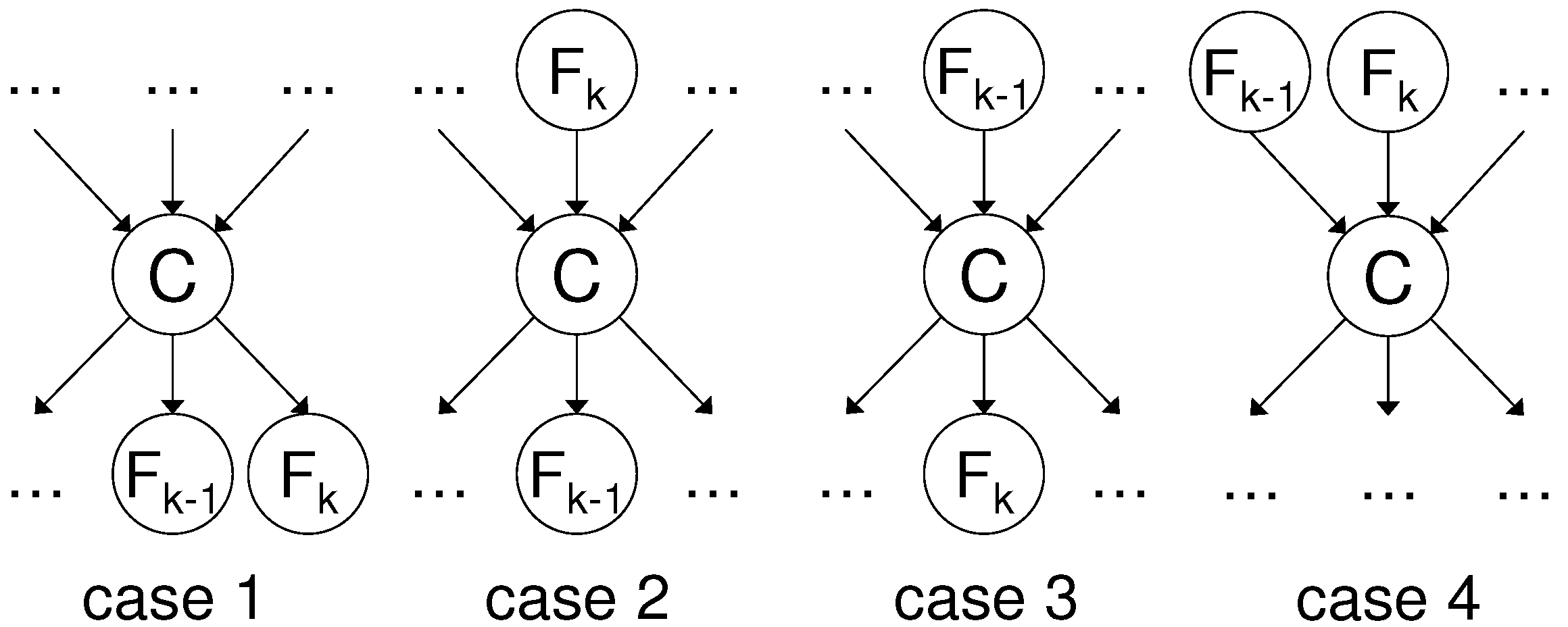
Next, we ask ourselves under what condition the decreasing returns holds. Suppose that the selected subset found so far is S, and that the feature selected in the current iteration is F${}_x$. In order for the decreasing returns to hold, one requires for the next selected feature F${}_y$: MI(F${}_x$;C∣S) > MI(F${}_y$;C∣ S,F${}_x$). First, we expand MI(F${}_x$,F${}_y$;C∣ S) in two ways by means of the chain rule of information:

$$\begin{array}{ccc}\hfill MI(F_x,F_y;C|\mathit{S})& =& MI(F_x;C|\mathit{S})+MI(F_y;C|\mathit{S},F_x)\hfill \\ & =& MI(F_y;C|\mathit{S})+MI(F_x;C|\mathit{S},F_y)\hfill \end{array}$$

(22)

In the sequential forward search, F${}_x$ was selected before F${}_y$, thus, it must be that: MI(F${}_x$;C∣S) > MI(F${}_y$;C∣S). In the case of ties, it may be possible that MI(F${}_x$;C∣S) ≥ MI(F${}_y$;C∣S), we focus here on the case where we have a strict ordering >. Then, in Equation (22) we have that:

$$\begin{array}{c}\hfill MI(F_y;C|\mathit{S},F_x)<MI(F_x;C|\mathit{S},F_y)\end{array}$$

(23)

Hence, a sufficient condition in order for the decreasing returns to hold is that: MI(F${}_x$;C∣S,F${}_y$) ≤ MI(F${}_x$;C∣S). This means that additional conditioning on F${}_y$ decreases (or equals) information of F${}_x$ about C.

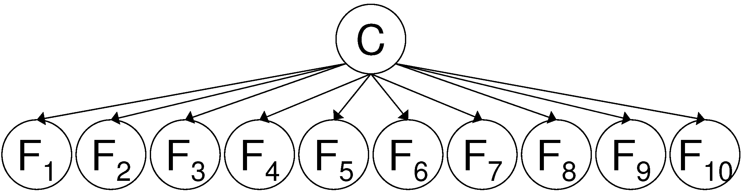
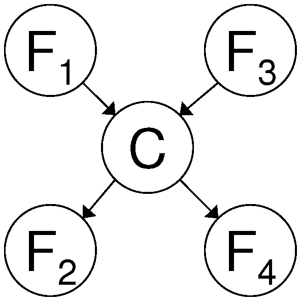
A first dependency structure between variables for which the decreasing returns can be proven to hold in the SFS is when all features are child nodes of the class variable C. This means that all features are conditionally independent given the class variable. This dependency structure is shown in Figure 4.

Lemma 4.1. 

Suppose that the order in which features are selected by the SFS is: firstly F${}_1$ subsequently F${}_2$ next F${}_3$ until F${}_n$. If all features are conditionally independent given the class variable, i.e. p(F${}_1$,F${}_2$, …F${}_n$∣C) = ${\prod }_{i=1}^n$ p(F${}_i$∣C), then the decreasing returns behavior holds: MI(F${}_1$;C) > MI(F${}_2$;C∣F${}_1$) > MI(F${}_3$;C∣F${}_1$,F${}_2$) > … > MI(F${}_n$;C∣F${}_1$,F${}_2$…F${}_{n-1}$).

Proof. 

First, we show that MI(F${}_1$;C) > MI(F${}_2$;C∣F${}_1$).

$$\begin{array}{ccc}\hfill MI(F_2;F_1,C)& =& MI(F_2;C)+MI(F_2;F_1|C)\hfill \end{array}$$

(24)

$$\begin{array}{ccc}& =& MI(F_2;F_1)+MI(F_2;C|F_1)\hfill \end{array}$$

(25)

In Equation (24) it holds that, due to the conditional independence of the features given the class variable, MI(F${}_2$;F${}_1$∣C) = 0. In Equation (25), we have that MI(F${}_2$;F${}_1$) ≥ 0. Comparing Equations (24) and (25), we obtain that: MI(F${}_2$;C) ≥ MI(F${}_2$;C∣F${}_1$). Because, F${}_1$ was selected before F${}_2$, we have that MI(F${}_1$;C) > MI(F${}_2$;C) (again we assume a strict ordering among variables, in case of ties we have MI(F${}_1$;C) ≥ MI(F${}_2$;C)). Hence, we obtain MI(F${}_1$;C) > MI(F${}_2$;C) ≥ MI(F${}_2$;C∣F${}_1$).

Using a similar reasoning as above, we can show that it holds in general: MI(F${}_{k-1}$;C∣F${}_1$,F${}_2$,…F${}_{k-2}$) > MI(F${}_k$;C∣F${}_1$,F${}_2$,…F${}_{k-1}$). We start with the generalization of Equation (24):

$$\begin{array}{ccc}\hfill MI(F_k;F_1,F_2,\dots F_{k-1},C)& =& MI(F_k;F_1,F_2,\dots F_{k-2},C)+MI(F_k;F_{k-1}|C,F_1,\dots F_{k-2})\hfill \end{array}$$

(26)

In appendix (B), we prove that the conditional independence of the variables given C implies that MI(F${}_k$;F${}_{k-1}$∣C,F${}_1$,…F${}_{k-2}$) = 0. Further expansion of the left and the right hand sides in Equation (26) results in:

$$\begin{array}{ccc}\hfill MI(F_k;F_1,F_2,\dots F_{k-1},C)& =& MI(F_k;F_1,F_2,\dots F_{k-2},C)\hfill \end{array}$$

(27)

$$\begin{array}{ccc}\hfill MI(F_k;F_1,\dots F_{k-1})+MI(F_k;C|F_1,\dots F_{k-1})& =& MI(F_k;F_1,\dots F_{k-2})+MI(F_k;C|F_1,\dots F_{k-2})\hfill \end{array}$$

(28)

Because MI(F${}_k$;F${}_1$,…F${}_{k-1}$) ≥ MI(F${}_k$;F${}_1$,…F${}_{k-2}$) in Equation (28), we see that MI(F${}_k$;C∣F${}_1$,…F${}_{k-1}$) ≤ MI(F${}_k$;C∣F${}_1$,…F${}_{k-2}$). But, F${}_{k-1}$ was selected before F${}_k$, i.e. MI(F${}_k$;C∣F${}_1$,…F${}_{k-2}$) < MI(F${}_{k-1}$;C∣F${}_1$,…F${}_{k-2}$), from which we obtain what needed to be proven: MI(F${}_k$;C∣F${}_1$,…F${}_{k-1}$) < MI(F${}_{k-1}$;C∣F${}_1$,…F${}_{k-2}$). ☐

In Figure 4 we show a Bayesian network [19,20] where the class variable C has 10 child nodes. This network has 21 degrees of freedom: we can randomly choose p(c=0) ∈ [0,1] and for the features we can choose p(f${}_i$=0∣c=0) ∈ [0,1] and p(f${}_i$=0∣c=1) ∈ [0,1]. We generated a Bayesian network where the probability p(c=0) and the conditional probabilities p(f${}_i$=0∣c=0) and p(f${}_i$=0∣c=1) are generated randomly following a uniform distribution within [0,1]. According to Lemma 4.1, we should find the decreasing returns behavior if we apply the SFS to this network.

Figure 4. Example of class conditional independence of the features given the class variable C. The joint probability distribution can be factorized as: p(F${}_1$,F${}_2$,…F${}_{10}$,C) = (${\prod }_{i=1}^{10}$ p(F${}_i$∣C)).p(C).

Figure 4. Example of class conditional independence of the features given the class variable C. The joint probability distribution can be factorized as: p(F${}_1$,F${}_2$,…F${}_{10}$,C) = (${\prod }_{i=1}^{10}$ p(F${}_i$∣C)).p(C).

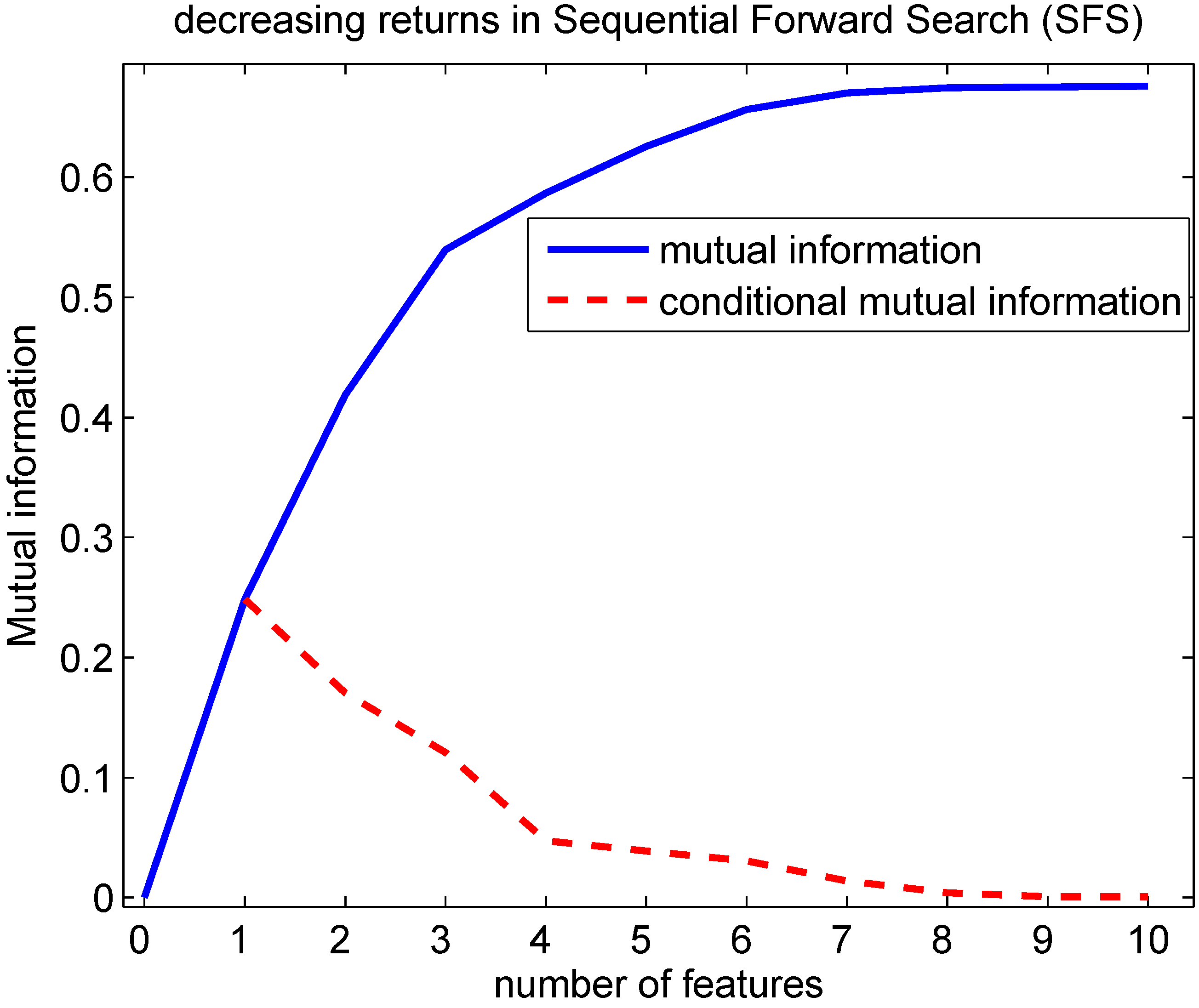
Indeed, this decreasing returns behavior can be observed in Figure 5 using the generated Bayesian network: Lemma 4.1 predicts that the conditional mutual information decreases with an increasing number of features being selected. This implies that the mutual information is a concave function in function of the number of features selected. This can be seen from the fact that the mutual information can be written as a sum of conditional mutual information terms:

$$\begin{array}{cc}& MI(F_1,F_2,\dots F_n;C)=MI(F_1;C)+M(F_2;C|F_1)+\dots +MI(F_n;C|F_1,F_2,\dots F_{n-1})\end{array}$$

(29)

with every next term smaller than the previous one. A particular case of Figure 4 is obtained if besides class conditional independence among features also independence is assumed. In that case, it can be shown [21] that the high-dimensional mutual information, can be written as a sum of marginal information contributions:

$$\begin{array}{cc}& MI(F_1,F_2,\dots F_n;C)=MI(F_1;C)+M(F_2;C)+\dots +MI(F_n;C)\end{array}$$

(30)

The SFS, which is in general not optimal, can then be shown to be optimal in mutual information sense. Indeed, at the k’th step of the SFS, i.e. after ‘k’ features have been selected, there is no subset of ‘k’ or less than ‘k’ features out of the set of ‘n’ features that leads to a higher mutual information than the set that has been found with the SFS at step ‘k’, if MI(F${}_k$;C) > 0. Independence and class conditional independence will often not be satisfied for data sets. Nevertheless, for gene expression data sets that typically contain up to 10,000 features, overfitting in a wrapper search can be alleviated if the features with the lowest mutual information are removed before applying the wrapper search [22].

Figure 5. Evolution of the mutual information in function of the number of features selected with the SFS. A Bayesian network according to Figure 4 was created with probability p(c=0), conditional probabilities p(f${}_i$=0∣c=0) and p(f${}_i$=0∣c=1) drawn randomly following a uniform distribution within [0,1]. The conditional mutual information at 1 feature is MI(F${}_1$;C) at 2 features MI(F${}_2$;C∣F${}_1$),… and finally at 10 features MI(F${}_{10}$;C∣F${}_1$,F${}_2$,…F${}_9$). Lemma 4.1 predicts that the conditional mutual information decreases with an increasing number of features selected. This implies that the mutual information is concave in function of the number of features selected.

Figure 5. Evolution of the mutual information in function of the number of features selected with the SFS. A Bayesian network according to Figure 4 was created with probability p(c=0), conditional probabilities p(f${}_i$=0∣c=0) and p(f${}_i$=0∣c=1) drawn randomly following a uniform distribution within [0,1]. The conditional mutual information at 1 feature is MI(F${}_1$;C) at 2 features MI(F${}_2$;C∣F${}_1$),… and finally at 10 features MI(F${}_{10}$;C∣F${}_1$,F${}_2$,…F${}_9$). Lemma 4.1 predicts that the conditional mutual information decreases with an increasing number of features selected. This implies that the mutual information is concave in function of the number of features selected.

It can be shown that also in more complex settings when there are both child and parent nodes the decreasing returns behavior can still hold. In Figure 6 an example of dependencies between 4 features is provided for which the decreasing returns holds, if the parent and child nodes are selected alternately. This leads to the following lemma.

Figure 6. Example of dependencies between features for decreasing returns. The joint probability distribution can be factorized as: p(F${}_1$,F${}_2$,F${}_3$,F${}_4$,C) = p(F${}_2$∣C).p(F${}_4$∣C).p(C∣F${}_1$,F${}_3$) .p(F${}_1$).p(F${}_3$). This factorization implies that: MI(F${}_1$,F${}_3$;F${}_2$,F${}_4$∣C) = 0.

Figure 6. Example of dependencies between features for decreasing returns. The joint probability distribution can be factorized as: p(F${}_1$,F${}_2$,F${}_3$,F${}_4$,C) = p(F${}_2$∣C).p(F${}_4$∣C).p(C∣F${}_1$,F${}_3$) .p(F${}_1$).p(F${}_3$). This factorization implies that: MI(F${}_1$,F${}_3$;F${}_2$,F${}_4$∣C) = 0.

Lemma 4.2. 

Suppose that the order in which features are selected by the SFS is: firstly F${}_1$ subsequently F${}_2$ next F${}_3$ until F${}_n$. Assume that the odd selected features,i.e.F${}_1$, F${}_3$, F${}_5$ …, are parents of C and the even selected features,i.e.F${}_2$, F${}_4$, F${}_6$ …, are children of C, then the decreasing returns behavior holds: MI(F${}_1$;C) > MI(F${}_2$;C∣F${}_1$) > MI(F${}_3$;C∣F${}_1$,F${}_2$) > … > MI(F${}_n$;C∣F${}_1$,F${}_2$,…F${}_{n-1}$).

Let us first prove the result for the case with 4 features, as shown in Figure 6. The order of selected features in the SFS is F${}_1$, F${}_2$, F${}_3$ and F${}_4$, respectively. We show that MI(F${}_3$;C∣F${}_1$,F${}_2$) < MI(F${}_2$;C∣F${}_1$).

$$\begin{array}{ccc}\hfill MI(F_3;C,F_1,F_2)& =& MI(F_3;F_1,F_2)+MI(F_3;C|F_1,F_2)\hfill \end{array}$$

(31)

$$\begin{array}{ccc}& =& MI(F_3;F_1)+MI(F_3;C|F_1)+MI(F_3;F_2|C,F_1)\hfill \end{array}$$

(32)

In Equation (32) MI(F${}_3$;F${}_2$∣C,F${}_1$) = 0, this follows from the fact that MI(F${}_1$,F${}_3$;F${}_2$,F${}_4$∣C) = 0, see appendix (A). We have in Equation (31) and Equation (32) that MI(F${}_3$;F${}_1$,F${}_2$) ≥ MI(F${}_3$;F${}_1$). Hence, combining previous 2 results yields: MI(F${}_3$;C∣F${}_1$,F${}_2$) ≤ MI(F${}_3$;C∣F${}_1$). Because feature F${}_2$ is selected before F${}_3$ we have: MI(F${}_2$;C∣F${}_1$) > MI(F${}_3$;C∣F${}_1$). Finally, we obtain that MI(F${}_3$;C∣F${}_1$,F${}_2$) < MI(F${}_2$;C∣F${}_1$). Similar expansions for MI(F${}_2$;C,F${}_1$) and MI(F${}_4$;C,F${}_1$,F${}_2$,F${}_3$) as in Equations (31) and (32), enable us to prove that MI(F${}_2$;C∣F${}_1$) < MI(F${}_1$;C) and MI(F${}_4$;C∣F${}_1$,F${}_2$,F${}_3$) < MI(F${}_3$;C∣F${}_1$,F${}_2$) respectively. Hence, we can conclude that the decreasing returns holds.

Now let us prove the result for any ‘k’ in general and regardless whether F${}_k$ is a parent node or a child node. Apply a similar expansion as in Equation (31).

$$\begin{array}{ccc}\hfill MI(F_k;C,F_1,F_2,\dots F_{k-1})& =& MI(F_k;F_1,F_2,\dots F_{k-1})+MI(F_k;C|F_1,F_2,\dots F_{k-1})\hfill \\ & =& MI(F_k;F_1,F_2,\dots F_{k-2})+MI(F_k;C|F_1,F_2,\dots F_{k-2})\hfill \end{array}$$

(33)

$$\begin{array}{ccc}& & +MI(F_k;F_{k-1}|C,F_1,\dots F_{k-2})\hfill \end{array}$$

(34)

Comparing Equations (33) and (34), we have that: MI(F${}_k$;F${}_1$,F${}_2$,…F${}_{k-1}$) ≥ MI(F${}_k$;F${}_1$,F${}_2$,…F${}_{k-2}$). Moreover, in Equation (34): MI(F${}_k$;F${}_{k-1}$∣C,F${}_1$,…F${}_{k-2}$) = 0, due to the fact that parent and child nodes are independent when conditioned on C. Hence, we conclude that MI(F${}_k$;C∣F${}_1$,F${}_2$,…F${}_{k-1}$) ≤ MI(F${}_k$;C∣F${}_1$,F${}_2$,…F${}_{k-2}$). Because F${}_{k-1}$ was selected before F${}_k$, we have that MI(F${}_k$;C∣F${}_1$,F${}_2$,…F${}_{k-2}$) < MI(F${}_{k-1}$;C∣F${}_1$,F${}_2$,…F${}_{k-2}$). Hence, finally this yields what is to be proven: MI(F${}_k$;C∣F${}_1$,F${}_2$,…F${}_{k-1}$) < MI(F${}_{k-1}$;C∣F${}_1$,F${}_2$,…F${}_{k-2}$). Note that we did not need to specify whether F${}_k$ is a parent or a child node, we only needed that one node F${}_k$ or F${}_{k-1}$ was a parent node and the other a child node.

Because, the proof is independent regardless F${}_k$ is a child or a parent node, we obtain following corollary of Lemma 4.2.

Corollary 4.3. 

Suppose that the order in which features are selected by the SFS is: firstly F${}_1$ subsequently F${}_2$ next F${}_3$ until F${}_n$. Assume that the odd selected features,i.e.F${}_1$, F${}_3$, F${}_5$ …, are children of C and the even selected features,i.e.F${}_2$, F${}_4$, F${}_6$ …, are parents of C, then the decreasing returns behavior holds: MI(F${}_1$;C) > MI(F${}_2$;C∣F${}_1$) > MI(F${}_3$;C∣F${}_1$,F${}_2$) > … > MI(F${}_n$;C∣F${}_1$,F${}_2$,…F${}_{n-1}$).

We performed an experiment to verify whether it is plausible that parent and child nodes may become selected alternately in the SFS, as Lemma 4.2 and Corollary 4.3 require. We generated 10,000 Bayesian networks with 2 parent and 2 child nodes as shown in Figure 6. This network contains 10 degrees of freedom. The following probabilities can be chosen freely: the prior probabilities p(f${}_1$=0) and p(f${}_3$=0), the conditional probability p(c=0∣f${}_1$,f${}_3$) for all 4 combinations of F${}_1$ and F${}_3$, p(f${}_2$=0∣c) for the 2 values of C and p(f${}_4$=0∣c) for the 2 values of C. In each of the 10,000 networks, probabilities were drawn following a uniform distribution within [0,1]. It can be shown that randomly assigning conditional distributions in this way, this will result almost always in joint distributions that are faithful to the directed acyclic graph (DAG). This means that no conditional independencies are present in the joint distribution that are not entailed by the DAG based on the Markov condition, see e.g., [20] on page 99. Next, the SFS was applied to each of the 10,000 networks. In 943 out of 10,000 cases, a parent node was selected first and parent and child nodes were selected alternately. In 1,125 out of 10,000 cases, a child node was selected first and parent and child nodes were selected alternately. In Table 2 we show the probabilities of a Bayesian network in which first a parent node was selected and the parent and child nodes were selected alternately. The evolution of the mutual information, when the SFS is applied to the Bayesian network with probabilities shown in Table 2, is shown in Figure 7.

4.3. Selection Transitions

We show that Lemmas 4.1 and 4.2 and Corollary 4.3 can be put in a more global theory of allowed selection transitions between features to achieve a decrease in return. When the target variable has both parent and child features, four elementary selection transitions can occur as shown in Figure 8.

Lemma 4.4. 

Suppose that feature F${}_k$ is just selected after feature F${}_{k-1}$ in the SFS. Assume a network with child and parent variables of the target variable C as shown in Figure 8 then a decrease in return must hold, i.e. MI(F${}_k$;C∣F${}_1$,F${}_2$,…F${}_{k-1}$) < MI(F${}_{k-1}$;C∣F${}_1$,F${}_2$,…F${}_{k-2}$), in: case 1) F${}_{k-1}$ is a child node and F${}_k$ is a child node, in case 2) F${}_{k-1}$ is a child node and F${}_k$ is a parent node and case 3) F${}_{k-1}$ is a parent node and F${}_k$ is a child node.

Proof. 

Case (1) F${}_{k-1}$ is a child node and F${}_k$ is a child node. The proof proceeds in a similar way as in Lemma 4.2 by starting from the same expansions as in Equations (33) and (34). If F${}_k$ and F${}_{k-1}$ are both child nodes then it can be proven that MI(F${}_k$;F${}_{k-1}$∣C,F${}_1$,…F${}_{k-2}$) = 0, holds, even in the case when there are parent nodes. This is shown in Appendix C. For the rest, the proof proceeds the same as in Lemma 4.2.

Case (2) F${}_{k-1}$ is a child node and F${}_k$ is a parent node. This result was already obtained at the end of the proof of Lemma 4.2 starting from Equations (33) and (34).

Case (3) F${}_{k-1}$ is a parent node and F${}_k$ is a child node. This result was already obtained at the end of the proof of Lemma 4.2 starting from Equations (33) and (34). ☐

Table 2. Probabilities for the network shown in Figure 6. These probabilities were obtained from one of the 10,000 Bayesian networks that were generated randomly. Applying the SFS to the network with these probabilities leads to the selection of parent and child nodes alternately.

F${}_1$	F${}_2$	F${}_3$	F${}_4$	C	p(.)
0					p(F${}_1$) = 0.6596
1					p(F${}_1$) = 0.3404
		0			p(F${}_3$) = 0.5186
		1			p(F${}_3$) = 0.4814
0		0		0	p(C∣F${}_1$,F${}_3$) = 0.9730
0		0		1	p(C∣F${}_1$,F${}_3$) = 0.0270
1		0		0	p(C∣F${}_1$,F${}_3$) = 0.6490
1		0		1	p(C∣F${}_1$,F${}_3$) = 0.3510
0		1		0	p(C∣F${}_1$,F${}_3$) = 0.8003
0		1		1	p(C∣F${}_1$,F${}_3$) = 0.1997
1		1		0	p(C∣F${}_1$,F${}_3$) = 0.4538
1		1		1	p(C∣F${}_1$,F${}_3$) = 0.5462
	0			0	p(F${}_2$∣C) = 0.4324
	1			0	p(F${}_2$∣C) = 0.5676
	0			1	p(F${}_2$∣C) = 0.8253
	1			1	p(F${}_2$∣C) = 0.1747
			0	0	p(F${}_4$∣C) = 0.0835
			1	0	p(F${}_4$∣C) = 0.9165
			0	1	p(F${}_4$∣C) = 0.1332
			1	1	p(F${}_4$∣C) = 0.8668

Table 2. Probabilities for the network shown in Figure 6. These probabilities were obtained from one of the 10,000 Bayesian networks that were generated randomly. Applying the SFS to the network with these probabilities leads to the selection of parent and child nodes alternately.

F${}_1$	F${}_2$	F${}_3$	F${}_4$	C	p(.)
0					p(F${}_1$) = 0.6596
1					p(F${}_1$) = 0.3404
		0			p(F${}_3$) = 0.5186
		1			p(F${}_3$) = 0.4814
0		0		0	p(C∣F${}_1$,F${}_3$) = 0.9730
0		0		1	p(C∣F${}_1$,F${}_3$) = 0.0270
1		0		0	p(C∣F${}_1$,F${}_3$) = 0.6490
1		0		1	p(C∣F${}_1$,F${}_3$) = 0.3510
0		1		0	p(C∣F${}_1$,F${}_3$) = 0.8003
0		1		1	p(C∣F${}_1$,F${}_3$) = 0.1997
1		1		0	p(C∣F${}_1$,F${}_3$) = 0.4538
1		1		1	p(C∣F${}_1$,F${}_3$) = 0.5462
	0			0	p(F${}_2$∣C) = 0.4324
	1			0	p(F${}_2$∣C) = 0.5676
	0			1	p(F${}_2$∣C) = 0.8253
	1			1	p(F${}_2$∣C) = 0.1747
			0	0	p(F${}_4$∣C) = 0.0835
			1	0	p(F${}_4$∣C) = 0.9165
			0	1	p(F${}_4$∣C) = 0.1332
			1	1	p(F${}_4$∣C) = 0.8668

Let us remark that case (4) does not necessarily exclude a decreasing return. This occurs e.g., when the probability distribution is not faithful to the directed acyclic graph (DAG). In that case it occurs that MI(F${}_k$;F${}_{k-1}$∣C,F${}_1$,…F${}_{k-2}$) = 0 and hence the decreasing returns holds. This independence is not entailed by the DAG based on the Markov condition [20]. Now let us reinterpret Lemmas 4.1 and 4.2 and Corollary 4.3 in light of Lemma 4.4. Lemma 4.1 only consists of the selection transitions of case 1 and hence the decreasing returns is guaranteed. Lemma 4.2 starts with a parent, next a child is

Figure 7. Evolution of the mutual information in function of the number of features selected with the SFS. A Bayesian network according to Figure 6 was created with the probabilities set to values listed in Table 2. The conditional mutual information at 1 feature is MI(F${}_1$;C) at 2 features MI(F${}_2$;C∣F${}_1$),… and finally at 4 features MI(F${}_4$;C∣F${}_1$,F${}_2$,F${}_3$). Lemma 4.2 predicts that the conditional mutual information decreases with an increasing number of features selected. This implies that the mutual information is concave in function of the number of features selected.

Figure 7. Evolution of the mutual information in function of the number of features selected with the SFS. A Bayesian network according to Figure 6 was created with the probabilities set to values listed in Table 2. The conditional mutual information at 1 feature is MI(F${}_1$;C) at 2 features MI(F${}_2$;C∣F${}_1$),… and finally at 4 features MI(F${}_4$;C∣F${}_1$,F${}_2$,F${}_3$). Lemma 4.2 predicts that the conditional mutual information decreases with an increasing number of features selected. This implies that the mutual information is concave in function of the number of features selected.

Figure 8. Four elementary selection transitions in the SFS. F${}_{k-1}$ is the feature selected at step k-1, F${}_k$ is the feature selected at step k. Case 1: F${}_{k-1}$ is a child and F${}_k$ is a child. Case 2: F${}_{k-1}$ is a child and F${}_k$ is a parent. Case 3: F${}_{k-1}$ is a parent and F${}_k$ is a child. Case 4: F${}_{k-1}$ is a parent and F${}_k$ is a parent.

Figure 8. Four elementary selection transitions in the SFS. F${}_{k-1}$ is the feature selected at step k-1, F${}_k$ is the feature selected at step k. Case 1: F${}_{k-1}$ is a child and F${}_k$ is a child. Case 2: F${}_{k-1}$ is a child and F${}_k$ is a parent. Case 3: F${}_{k-1}$ is a parent and F${}_k$ is a child. Case 4: F${}_{k-1}$ is a parent and F${}_k$ is a parent.

selected (i.e., a case 3 transition), next a parent is selected (i.e., a case 2 transition) and so on. Hence, case 3 and case 2 transitions are alternated. Corollary 4.3, starts with a child, next a parent is selected (i.e., a case 2 transition), next a child is selected (i.e., a case 3 transition) and so on. Hence case 2 and case 3 transitions are alternated. Let us remark that also other combinations of cases are possible to guarantee the decreasing returns behavior. A case 3 (parent → child) transition is also allowed to be followed by a case 1 transition (child → child), and a case 1 (child → child) transition is allowed to be followed by a case 2 (child → parent) transition. Finally, we remark that the increasing returns behavior illustrated by the XOR hypercube in Section 4.1 is an example of case 4 transitions.

4.4. Relevance-redundancy Criteria

To avoid the estimation of mutual information in high-dimensional spaces, Battiti [11] proposed a SFS criterion that selects in each iteration the feature with the largest marginal relevance penalized with a redundancy term. Suppose that the set of features selected thus far is S and that F${}_i$ is a candidate feature to be selected, then the feature F${}_i$ is selected for which following criterion is maximal.

$$\begin{array}{c}\hfill Crit=MI(F_i;C)-\beta \sum _{F_s\in \mathit{S}}\alpha (F_i,F_s,C)MI(F_i;F_s)\end{array}$$

(35)

In Battiti’s work $\beta$ is a user defined parameter and $\alpha$ (F${}_i$,F${}_s$,C) = 1. Similar criteria were proposed in [23] (for which $\alpha$ (F${}_i$,F${}_s$,C) = $\frac{MI(F_s;C)}{H(F_s)}$), in [24] (for which $\alpha$ (F${}_i$,F${}_s$,C) = 1 and $\beta$ is adaptively chosen as 1/∣S∣) and in [25] (for which $\alpha$ (F${}_i$,F${}_s$,C) = 1/min{H(F${}_i$),H(F${}_s$)} and $\beta$ is adaptively chosen as 1/∣S∣). All these criteria will not be informative for the examples shown in Section 3.1, Section 3.2 and Section 3.3. These criteria will return for each feature in Equation (35) Crit = 0, because MI(F${}_i$;C) = 0 and MI(F${}_i$;F${}_s$) = 0. Therefore, these criteria may be tempted to include no features at all, despite the fact that all features are strongly relevant. For the 7-5-3 XOR cube all criteria will select the features in the same order: first F${}_1$, then F${}_2$ and then F${}_3$. This is due to the fact that F${}_1$ individually contains more information than F${}_2$ about the target variable, see Table 1. Also F${}_2$ contains more information than F${}_3$ about the target variable, see Table 1. Moreover for the 7-5-3 XOR cube all variables are independent, hence MI(F${}_i$;F${}_s$) = 0. However, from the criterion values Crit = MI(F${}_1$;C), then Crit = MI(F${}_2$;C) and finally Crit = MI(F${}_3$;C) the increasing returns cannot be observed. Another criterion that uses lower-dimensional conditional mutual information to select features was proposed in [26]. This selection algorithm proceeds in 2 stages:

$$\begin{array}{ccc}& & F_{s1}=\underset{1\le i\le n}{arg\; max}MI(F_i;C)\hfill \end{array}$$

(36)

$$\begin{array}{ccc}& & F_{sk}=\underset{j}{arg\; max}\left\{\underset{1\le i\le k-1}{min}MI(F_j;C|F_{si})\right\}\hfill \end{array}$$

(37)

In the first step in Equation (36) the feature which bears individually most information about the target variable is selected, i.e., F${}_{s1}$. Next, in the k’th step of the second stage, i.e., Equation (37), the feature is selected which contributes most, conditioned on the set of already selected features F${}_{s1}$, F${}_{s2}$, …F${}_{sk-1}$. The contribution for feature F${}_j$ is estimated conservatively as ${min}_{1\le i\le k-1}MI(F_j;C|F_{si})$. This algorithm will be able to detect the increasing returns in the XOR problem in case there are only 2 features. However, it would fail to detect the strongly relevant features in case there are at least 3 features in the XOR problem. To overcome the limitations of the lower-dimensional mutual information estimators, higher-dimensional mutual information estimators for classification purposes were proposed [21,22,27,28]. In [27] the authors proposed a density-based method: the probability density is estimated by means of Parzen windows and the mutual information is estimated from this probability density estimate. In [21,22] the mutual information was estimated based on pair-wise distances between data points. A similar estimator can be used for regression purposes [29]. In [28] the mutual information is estimated also based on distances between data points, but this time from a minimal spanning tree that is constructed from the data points.

4.5. Importance of Increasing and Decreasing Returns

The importance of the decreasing and increasing returns lies in that we can compute an upper bound and a lower bound on the probability of error, without having to compute the mutual information for higher dimensions. Suppose that the mutual information has been computed up to a subset of $n1$ features F${}_{n1}$, with mutual information MI(F${}_{n1}$;C). Suppose that the last increment in going from a subset of $n1-1$ features F${}_{n1-1}$ to F${}_{n1}$ equals ΔMI = MI(F${}_{n1}$;C)-MI(F${}_{n1-1}$;C). For the mutual information of a subset of n2 features F${}_{n2}$, with F${}_{n2}$ ⊃ F${}_{n1}$, it holds, under the decreasing returns, that:

$$\begin{array}{cc}& MI({\mathit{F}}_{n1};C)\le \end{array}$$

$$\begin{array}{cc}& MI({\mathit{F}}_{n2};C)\le MI({\mathit{F}}_{n1};C)+(|n2|-\left|n1\right|)\Delta MI\end{array}$$

(38)

and under the increasing returns that:

$$\begin{array}{c}\hfill MI({\mathit{F}}_{n2};C)\ge MI({\mathit{F}}_{n1};C)+(|n2|-\left|n1\right|)\Delta MI\end{array}$$

(39)

For the example shown in Figure 5, it can be seen that ΔMI (the conditional mutual information) at 4 features is representative for the conditional mutual information at 5, 6 and 7 features. The conditional mutual information at 8 features is representative for the ones at 9 and 10 features. 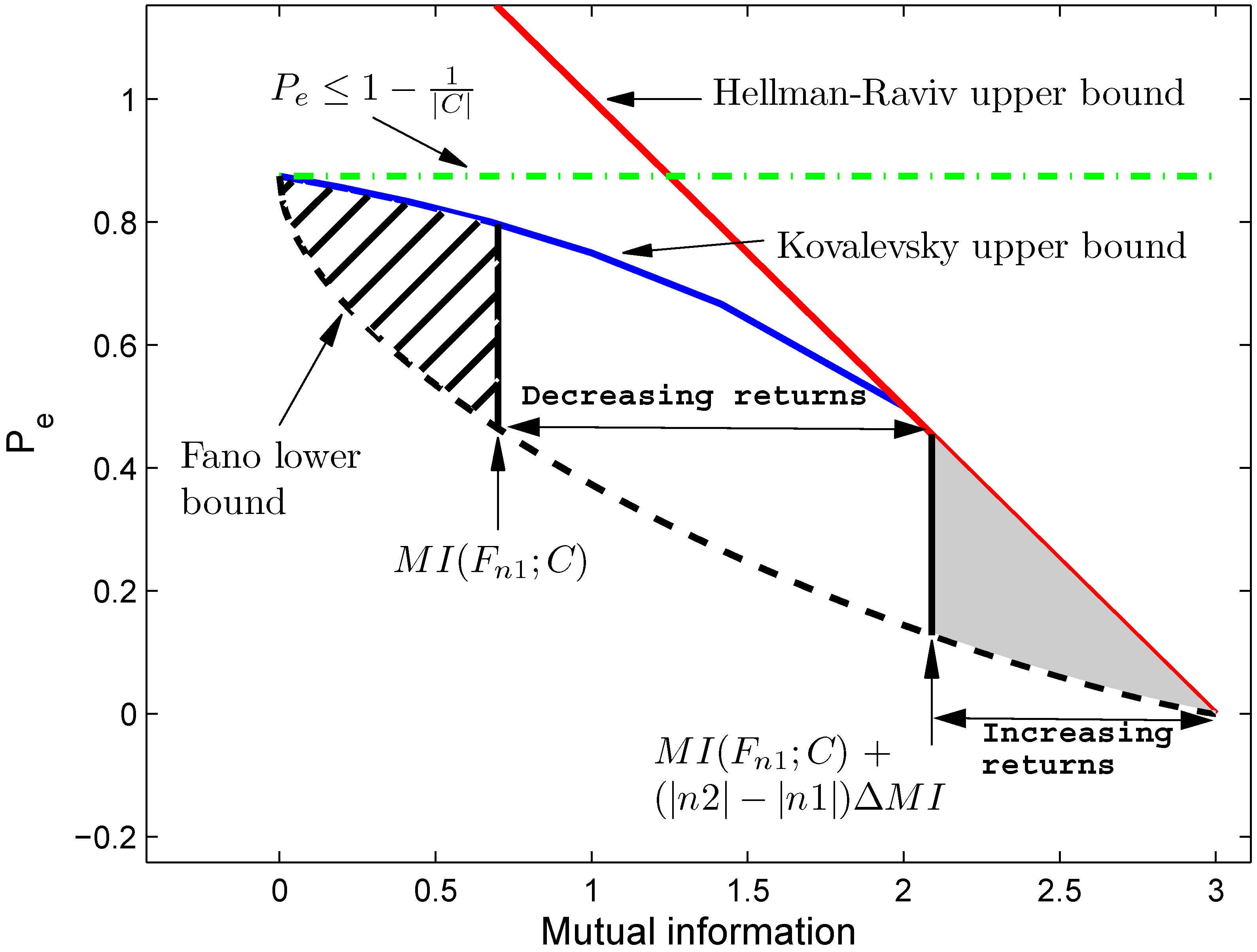From the inequalities in (38) and (39) one can constrain the probability of error that can be achieved by observing the ($\left|n2\right|$-$\left|n1\right|$) additional features. This can be obtained by exploiting upper and lower bounds that were established for the equivocation H(C∣F). These upper and lower bounds can be restated in terms of the mutual information. In Figure 9 the upper bounds are restated in terms of the mutual information as follows for the Hellman-Raviv upper bound [30]:

$$\begin{array}{c}\hfill \frac{(H(C)-MI(F;C))}{2}\ge P_e\end{array}$$

(40)

and for the Kovalevsky upper bound [31]:

$$\begin{array}{cc}& H(C)-MI(F;C)\ge \\ \hfill & lo{g}_2(i)+i(i+1)(lo{g}_2\frac{i+1}{i})(P_e-\frac{i-1}{i})\end{array}$$

(41)

with ‘i’ an integer such that ($i-1$)/i≤ P${}_e$≤ i/($i+1$) and ‘i’ smaller than the number of classes ∣C∣. Let us remark that some of the bounds on the probability of error have been established independently by different researchers. The Hellman-Raviv upper bound has also been found in [32]. The Kovalevsky upper bound on the probability of error has been proposed at least 3 times: first in [31,32] and later in [33]; see also the discussion in [34]. The lower bound in Figure 9 is solved using the Fano lower bound [12,35]:

$$\begin{array}{c}\hfill H(C)-MI(F;C)\le H(P_e)+P_{e}lo{g}_2(\mid C\mid -1)\end{array}$$

(42)

Due to (38) it must be that the probability of error corresponding with F${}_{n2}$ falls within the white area under the decreasing returns, and, due to (39), within the dark grey area under the increasing returns.

Figure 9. Bounds on the probability of error. For subset F${}_{n1}$ the mutual information equals MI(F${}_{n1}$;C), for which the probability of error falls between the Fano lower bound and the Kovalevsky upper bound. The white area represents the possible combinations of probability of error and mutual information for the decreasing returns in the selection of (∣n2∣-∣n1∣) additional features, because MI(F${}_{n2}$;C) ≤ MI(F${}_{n1}$;C) + (∣n2∣-∣n1∣)ΔMI. The grey area is the possible area for the increasing returns. The hatched area is not possible, because adding features can only increase the information. This figure illustrates the case when the number of classes ∣C∣ is equal to 8 and when all prior probabilities of the classes are equal.

Figure 9. Bounds on the probability of error. For subset F${}_{n1}$ the mutual information equals MI(F${}_{n1}$;C), for which the probability of error falls between the Fano lower bound and the Kovalevsky upper bound. The white area represents the possible combinations of probability of error and mutual information for the decreasing returns in the selection of (∣n2∣-∣n1∣) additional features, because MI(F${}_{n2}$;C) ≤ MI(F${}_{n1}$;C) + (∣n2∣-∣n1∣)ΔMI. The grey area is the possible area for the increasing returns. The hatched area is not possible, because adding features can only increase the information. This figure illustrates the case when the number of classes ∣C∣ is equal to 8 and when all prior probabilities of the classes are equal.

5. Decreasing Losses and Increasing Losses

We show that the increasing returns and the decreasing returns for the SFS has a comparable implication in the sequential backward search (SBS): the comparable behavior for the increasing returns is the decreasing losses in the SBS, the comparable behavior for the decreasing returns is the increasing losses in the SBS.

5.1. Decreasing Losses

In the SBS, the feature, for which the information loss is minimal, is removed in every iteration. Starting from the example in Figure 3, one computes the 3 information losses: MI(F${}_1$,F${}_2$,F${}_3$;C) − MI(F${}_2$,F${}_3$;C) = MI(F${}_1$;C∣F${}_2$,F${}_3$), MI(F${}_2$;C∣F${}_1$,F${}_3$) and MI(F${}_3$;C∣F${}_1$,F${}_2$). One then removes the feature F${}_i$ for which MI(F${}_i$;C∣F${}_j$,F${}_k$) is minimal. We show the computations of the mutual information for the 7-5-3 XOR cube in Table 3. In the SBS for this example, we first remove F${}_3$, because MI(F${}_3$;C∣F${}_1$,F${}_2$) is

Table 3. 7-5-3 XOR Cube. Mutual Information for the SBS.

Mutual Information	value(bit)
MI(F${}_1$,F${}_2$,F${}_3$;C)	≈ 0,9999
MI(F${}_1$;C∣F${}_2$,F${}_3$)	≈ 0,9852
MI(F${}_2$;C∣F${}_1$,F${}_3$)	≈ 0,9710
MI(F${}_3$;C∣F${}_1$,F${}_2$)	≈ 0,9183
MI(F${}_1$;C∣F${}_2$)	≈ 8,007.10${}^{-2}$
MI(F${}_2$;C∣F${}_1$)	≈ 7,850.10${}^{-2}$
MI(F${}_1$;C)	≈ 3,143.10${}^{-3}$

Table 3. 7-5-3 XOR Cube. Mutual Information for the SBS.

Mutual Information	value(bit)
MI(F${}_1$,F${}_2$,F${}_3$;C)	≈ 0,9999
MI(F${}_1$;C∣F${}_2$,F${}_3$)	≈ 0,9852
MI(F${}_2$;C∣F${}_1$,F${}_3$)	≈ 0,9710
MI(F${}_3$;C∣F${}_1$,F${}_2$)	≈ 0,9183
MI(F${}_1$;C∣F${}_2$)	≈ 8,007.10${}^{-2}$
MI(F${}_2$;C∣F${}_1$)	≈ 7,850.10${}^{-2}$
MI(F${}_1$;C)	≈ 3,143.10${}^{-3}$

the smallest information loss for the set of 3 features. Next F${}_2$ is removed, because MI(F${}_2$;C∣F${}_1$) is the smallest for sets of 2 features and, finally, feature F${}_1$ remains. Instead of the increasing returns in the SFS, we observe now ‘decreasing losses’ in the SBS: MI(F${}_3$;C∣F${}_1$,F${}_2$) ≈ 0,9183 > MI(F${}_2$;C∣F${}_1$) ≈ 7,850.10${}^{-2}$ > MI(F${}_1$;C) ≈ 3,143.10${}^{-3}$. The 7-5-3 XOR cube also illustrates that, for this type of problems, the SBS can outperform the SFS. The initial small increments in the SFS are close to 0 (in the order of 10${}^{-3}$): for small values, it may be tempting to stop the SFS too early. In XOR-type problems, when the number of values the features can take are even, e.g., in the 8-8-8 XOR cube, the situation is even worse. All increments in the SFS are equal to 0, except only in the last iteration of the SFS, a large increment in the mutual information is observed. In the SBS, this problem is not encountered. In the first iteration of the SBS, a large information loss is observed immediately (≈ 0,9183). One concludes immediately correctly that one should not remove any features at all.

5.2. Increasing Losses

Similar as in the case of decreasing returns in the SFS, it can be questioned under which conditions ‘increasing losses’ can be observed. Suppose that, in our SBS example, F${}_y$ is removed before F${}_x$. We can use the 2 expansions of (22). When F${}_y$ is removed before F${}_x$, it must be that: MI(F${}_y$;C∣S,F${}_x$) < MI(F${}_x$;C∣S,F${}_y$). Combining this inequality with (22), it is clear that: MI(F${}_x$;C∣S) > MI(F${}_y$;C∣S). Hence, under the condition that MI(F${}_y$;C∣S) ≥ MI(F${}_y$;C∣S,F${}_x$) one obtains an ‘increasing losses’ behavior: MI(F${}_x$;C∣S) > MI(F${}_y$;C∣S,F${}_x$).

Lemmas comparable to Lemma 4.1 and Lemma 4.2 are obtained for the SBS. For Lemma 4.1 this leads in the SBS to the following lemma.

Lemma 5.1 

Suppose that the order in which features are removed by the SBS is: firstly F${}_n$ subsequently F${}_{n-1}$ next F${}_{n-2}$ until F${}_1$. If all features are conditionally independent given the class variable, i.e., p(F${}_1$,F${}_2$, …F${}_n$∣C) = ${\prod }_{i=1}^n$ p(F${}_i$∣C), then the increasing losses behavior holds: MI(F${}_n$;C∣F${}_1$,F${}_2$,…F${}_{n-1}$) < MI(F${}_{n-1}$;C∣F${}_1$,F${}_2$,…F${}_{n-2}$) < MI(F${}_{n-2}$;C∣F${}_1$,F${}_2$,…F${}_{n-3}$) < … < MI(F${}_2$;C∣F${}_1$) < MI(F${}_1$;C).

The proof proceeds in a similar way as in Lemma 4.1, but starts from a different mutual information than Equation (26).

$$\begin{array}{ccc}\hfill MI(F_{k-1};F_1,F_2,\dots F_{k-2},F_k,C)& =& MI(F_{k-1};F_1,F_2,\dots F_{k-2},C)+MI(F_{k-1};F_k|C,F_1,F_2,\dots F_{k-2})\hfill \end{array}$$

(43)

Similar as in Lemma 4.1, it holds that: MI(F${}_{k-1}$;F${}_k$∣C,F${}_1$,F${}_2$,…F${}_{k-2}$) = 0. Further expanding of the left and the right hand sides of Equation (43) results in:

$$MI(F_{k-1};F_1,F_2,\dots F_{k-2},F_k,C)=MI(F_{k-1};F_1,F_2,\dots F_{k-2},C)$$

(44)

$$\begin{array}{ccc}\hfill MI(F_{k-1};F_1,F_2,\dots F_{k-2},F_k)+MI(F_{k-1};C|F_1,F_2,\dots F_{k-2},F_k)& =& MI(F_{k-1};F_1,F_2,\dots F_{k-2})\hfill \\ & +& MI(F_{k-1};C|F_1,F_2,\dots F_{k-2})\hfill \end{array}$$

(45)

Because MI(F${}_{k-1}$;F${}_1$,F${}_2$,…F${}_{k-2}$,F${}_k$) ≥ MI(F${}_{k-1}$;F${}_1$,F${}_2$,…F${}_{k-2}$) in Equation (45), we see that MI(F${}_{k-1}$;C∣F${}_1$,F${}_2$,…F${}_{k-2}$,F${}_k$) ≤ MI(F${}_{k-1}$;C∣F${}_1$,F${}_2$,…F${}_{k-2}$). But, F${}_k$ was removed before F${}_{k-1}$, i.e., MI(F${}_k$;C∣F${}_1$,F${}_2$,…F${}_{k-1}$) < MI(F${}_{k-1}$;C∣F${}_1$,F${}_2$,…F${}_{k-2}$,F${}_k$), from which we obtain what needed to be proven: MI(F${}_k$;C∣F${}_1$,F${}_2$,…F${}_{k-1}$) < MI(F${}_{k-1}$;C∣F${}_1$,F${}_2$,…F${}_{k-2}$).

We generated a Bayesian network as in Figure 4 with the free parameters randomly drawn following a uniform distribution within [0,1]. According to Lemma 5.1, we should find the increasing losses behavior if we apply the SBS to this network. The result of the SBS is shown in Figure 10.

Similar to Lemma 4.2 when there are both child and parent nodes this leads in the SBS to the following lemma.

Lemma 5.2. 

Suppose that the order in which features are removed by the SBS is: firstly F${}_n$ subsequently F${}_{n-1}$ next F${}_{n-2}$ until F${}_1$. Assume that odd removed features, F${}_{n-1}$, F${}_{n-3}$,…F${}_3$, F${}_1$, are parents of C and even removed features, F${}_n$, F${}_{n-2}$,…F${}_4$, F${}_2$, are children of C, then the increasing losses behavior holds: MI(F${}_n$;C∣F${}_1$,F${}_2$,…F${}_{n-1}$) < MI(F${}_{n-1}$;C∣F${}_1$,F${}_2$,…F${}_{n-2}$) < MI(F${}_{n-2}$;C∣F${}_1$,F${}_2$,…F${}_{n-3}$) < … < MI(F${}_2$;C∣F${}_1$) < MI(F${}_1$;C).

Proof. 

The proof proceeds similar as in Lemma 4.2, but starts from a slightly different mutual information then Equation (33).

$$\begin{array}{ccc}\hfill MI(F_{k-1};C,F_1,F_2,\dots F_{k-2},F_k)& =& MI(F_{k-1};F_1,F_2,\dots F_{k-2},F_k)+MI(F_{k-1};C|F_1,F_2,\dots F_{k-2},F_k)\hfill \end{array}$$

(46)

$$\begin{array}{ccc}& =& MI(F_{k-1};F_1,F_2,\dots F_{k-2})+MI(F_{k-1};C|F_1,F_2,\dots F_{k-2})\hfill \\ & & +MI(F_{k-1};F_k|C,F_1,\dots F_{k-2})\hfill \end{array}$$

(47)

We do not need to specify that F${}_k$ is a parent or a child node, we only need that one node F${}_k$ or F${}_{k-1}$ is a parent node and the other a child node. Comparing Equations (46) and (47), we have that: MI(F${}_{k-1}$;F${}_1$,F${}_2$,…F${}_{k-2}$,F${}_k$) ≥ MI(F${}_{k-1}$;F${}_1$,F${}_2$,…F${}_{k-2}$). Moreover in Equation (47) MI(F${}_{k-1}$;F${}_k$∣C,F${}_1$,…F${}_{k-2}$) = 0 due to the fact that parent and child nodes are independent when conditioned on C. Hence, we conclude that MI(F${}_{k-1}$;C∣F${}_1$,F${}_2$,…F${}_{k-2}$,F${}_k$) ≤ MI(F${}_{k-1}$;C∣F${}_1$,F${}_2$,…F${}_{k-2}$). Because F${}_k$ was removed before F${}_{k-1}$, we have that MI(F${}_k$;C∣F${}_1$,F${}_2$,…F${}_{k-1}$) < MI(F${}_{k-1}$;C∣F${}_1$,F${}_2$,…F${}_{k-2}$,F${}_k$). Hence, finally this yields what is to be proven: MI(F${}_k$;C∣F${}_1$,F${}_2$,…F${}_{k-1}$) < MI(F${}_{k-1}$;C∣F${}_1$,F${}_2$,…F${}_{k-2}$).

Figure 10. Evolution of the mutual information in function of the number of features selected with the SBS. A Bayesian network according to Figure 4 was created with probability p(c=0), conditional probabilities p(f${}_i$=0∣c=0) and p(f${}_i$=0∣c=1) drawn randomly from a uniform distribution within [0,1]. The conditional mutual information for 10 features is MI(F${}_{10}$;C∣F${}_1$,F${}_2$,…F${}_9$), for 9 features MI(F${}_9$;C∣F${}_1$,F${}_2$,…F${}_8$),… and, finally for 1 feature MI(F${}_1$;C). Lemma 5.1 predicts that the conditional mutual information increases with increasing number of features removed. This implies that the mutual information is concave in function of the number of features selected.

Figure 10. Evolution of the mutual information in function of the number of features selected with the SBS. A Bayesian network according to Figure 4 was created with probability p(c=0), conditional probabilities p(f${}_i$=0∣c=0) and p(f${}_i$=0∣c=1) drawn randomly from a uniform distribution within [0,1]. The conditional mutual information for 10 features is MI(F${}_{10}$;C∣F${}_1$,F${}_2$,…F${}_9$), for 9 features MI(F${}_9$;C∣F${}_1$,F${}_2$,…F${}_8$),… and, finally for 1 feature MI(F${}_1$;C). Lemma 5.1 predicts that the conditional mutual information increases with increasing number of features removed. This implies that the mutual information is concave in function of the number of features selected.

Similar to Corollary 3, we obtain following corollary in the SBS.

Corollary 5.3. 

Suppose that the order in which features are removed by the SBS is: firstly F${}_n$ subsequently F${}_{n-1}$ next F${}_{n-2}$ until F${}_1$. Assume that odd removed features, F${}_{n-1}$, F${}_{n-3}$,…F${}_3$, F${}_1$, are children of C and even removed features, F${}_n$, F${}_{n-2}$,…F${}_4$, F${}_2$, are parents of C, then the increasing losses behavior holds: MI(F${}_n$;C∣F${}_1$,F${}_2$,…F${}_{n-1}$) < MI(F${}_{n-1}$;C∣F${}_1$,F${}_2$,…F${}_{n-2}$) < MI(F${}_{n-2}$;C∣F${}_1$,F${}_2$,…F${}_{n-3}$) < … < MI(F${}_2$;C∣F${}_1$) < MI(F${}_1$;C).

Finally, we can relate Lemmas 5.1 and 5.2 and Corollary 5.3 to the allowed selection transitions of Section 4.3.

Lemma 5.4. 

Suppose that feature F${}_{k-1}$ is just removed after feature F${}_k$ has been removed in the SBS. Assume a network with child and parent variables of the target variable C as shown in Figure 8 then an increase in loss must hold,i.e.MI(F${}_k$;C∣F${}_1$,F${}_2$,…F${}_{k-1}$) < MI(F${}_{k-1}$;C∣F${}_1$,F${}_2$,…F${}_{k-2}$), in: case 1) F${}_{k-1}$ is a child node and F${}_k$ is a child node, in case 2) F${}_{k-1}$ is a child node and F${}_k$ is a parent node and case 3) F${}_{k-1}$ is a parent node and F${}_k$ is a child node.

Proof. 

The proof is obtained starting from the expansions in Equations (46) and (47). It holds for all 3 cases that MI(F${}_{k-1}$;F${}_k$∣C,F${}_1$,…F${}_{k-2}$) = 0, then the proof proceeds similar as in Lemma 5.2.

Interpreting Figure 8 now as ‘F${}_{k-1}$ is removed just after F${}_k$ has been removed’, following combinations can be made to guarantee an increasing losses behavior. Case 1 (child → child) can be followed by case 1 (child → child) and by case 3 (child → parent). Case 2 (parent → child) can be followed by case 1 (child → child) or by case 3 (child → parent). Case 3 (child → parent) can be followed by case 2 (parent → child).

6. Conclusions

This work contributes to a more thorough understanding of the evolution of the mutual information in function of the number of features that are selected in the sequential forward search (SFS) and in the sequential backward search (SBS) strategies. Conditioning on additional features can increase the mutual information about the target variable for discrete features (binary as well as non-binary) and continuous features. Increments in mutual information can become larger and larger in the sequential forward search, a behavior we described as ‘increasing returns’. An example of increasing returns was constructed using a $(2n+1)-(2n-1)-\dots -5-3$ XOR hypercube. It was shown that, when conditioning on additional variables reduces information about the target variable, then this is a sufficient condition for the decreasing returns to hold in the sequential forward search. We provided examples of dependencies between features and the target variable from which the decreasing returns behavior could be proven to occur. If features are conditionally independent given the target variable, the decreasing returns behavior is proven to be guaranteed. Even in the case of more complex dependencies, when there are both child and parent variables, the decreasing returns was proven to occur when parent and child variables would be selected alternately by the SFS. The analogous behaviors in the mutual information based SBS are: ‘decreasing losses’ and ‘increasing losses’. Similar to the SFS, if conditioning on additional variables reduces information about the target variable, then this is a sufficient condition for the increasing losses to hold in the SBS. If the features are conditionally independent given the target variable, the increasing losses behavior is proven to occur. If parent and child variables would be removed alternately by the SBS, the increasing losses behavior is also proven to occur. Lemmas were supported by experimental results.