Assessing the Information Content in Environmental Modelling: A Carbon Cycle Perspective

Abstract

A model represents the way in which information about the world is captured in a form that can be manipulated for application to new situations. However, quantification of ‘model error’ presents formidable challenges. Various inverse problems in carbon cycle modelling are presented as illustrations of the issues. A ‘maximum-entropy’ representation of carbon cycle response is used to explore techniques for non-parametric estimation of carbon cycle uncertainty.

1. Introduction

Model building is how science captures information about the world in a way that can be applied in new situations. It is highly desirable to be able to quantify the information content of models, in order to identify where the information is coming from. More specifically, we need to ensure that the information embodied in models reflects observations of the real world and not just mathematical convenience.

Bayes rule provides the basis for manipulating the accumulation of information from successive observations. This can be used for defining various measures of the information provided by observations although most applications express this in terms of reduction of variance, i.e. in terms appropriate for Gaussian distributions. One important distinction is between how much information is expected, on average, from a particular observation, and how much information is provided by the particular observed value. However, the difficulty with using Bayes rule is in defining a starting point. Bayesian estimation is often used in ‘model calibration’, i.e. tuning model parameters [1]. However such studies do not provide a measure of what is built in to the structure of the model — i.e. there is no quantification of ‘model error’.

While it is sometimes claimed that various forms of statistical modelling are shielded from such problems [2], a less partisan assessment is that the difficulties are ubiquitous across what Karplus [3] called the modelling spectrum. Parametric statistical modelling can be just as much a victim of built-in assumptions as process-based deterministic modelling.

The present paper explores these issues by considering aspects of the global carbon cycle. The case that is discussed in most detail is the decadal to century scale changes in atmospheric CO₂ in response to the emissions from fossil fuel use and from deforestation and other changes in land-use. In terms of statistical modelling, this is a non-stationary time series problem, i.e. one-dimensional, and is referred to as the 1-D problem. Synthetic examples of stationary time series are also used to illustrate particular issues. A number of specific issues of time series in carbon cycle studies have been described in [4].

As well as the 1-D problem, an additional example, termed the ‘2-D problem’, is that of deducing the mean spatial distribution of surface CO₂ fluxes from the surface distribution of CO₂ concentration. The generalisation to estimating the time-dependence of CO₂ fluxes is termed the (2+1)-D problem. These 2-D and (2+1)-D inverse problems form the topic of my book [5].

The various cases discussed in the present paper are intended to illustrate concepts that can be applied to more general uses of carbon cycle data that are not so readily classified. Some preliminary work on a ‘maximum entropy’ formulation of the decadal-to-century scale response of CO₂ concentrations to CO₂ emissions is used as an example of minimsing the contribution from ‘model error’ by using as few as possible parametric assumptions.

The outline of the remainder of this paper is as follows. Section 2 discusses the modelling spectrum described by Karplus [3] and the quantification of information in terms more general than the Gaussian ‘reduction in variance’ measure. Inverse problems are discussed in terms of statistical inference in Section 3. Section 4 applies these concepts to the analysis of how information is combined in carbon cycle modelling. The concluding remarks explore how these preliminary studies can be extended to a more comprehensive analysis of the way in which information is incorporated in the modelling process.

2. Modelling

2.1. A dichotomy

Before attempting to quantify the information content of models, it is useful to be more specific about the types of modelling that are involved. As a starting point, we consider a dichotomy that we term ‘curve fitting’ and ‘process modelling’. The basis of these approaches are:

• Curve Fitting :

  • Build model on basis of observed correlations between putative ‘inputs’ and ‘outputs’.
• Process modelling :

  • Build model on basis of ‘mechanistic’ relations between system components.

The main arguments, for and against these approaches, can be summarised as:

	Curve fitting	Process model
For	Formalism for analysing uncertainties	Wider range of validity
Against	No reason to assume validity beyond domain used for calibration	Vulnerable to neglect of processes – ‘Kelvin error’

The dichotomy has been discussed by Young and Garnier [2] in connection with their analysis of CO₂ stabilisation calculations of the type performed for the IPCC Radiative Forcing Report [6]. However, this discussion, promoting the benefits of their ‘data-based’ approach, has two related flaws. Firstly, in spite of their emphasis on data-based approaches, they ignore one of the most important data sets, the distributions of natural and anthropogenic ¹⁴C, from which understanding of the carbon cycle has been achieved. Secondly, when they note that mechanistic modelling tends to reflect modellers’ understanding, Young and Garnier fail to note that such understanding is based on incorporating a much wider body of observational data. It is this aspect, of being broadly data-based, and including using such observationally-based principles as conservation of mass, that gives mechanistic models the possibility of applicability beyond the types of data for which they were calibrated.

As noted in my more recent book [7], this dichotomy is playing a large role in public discussion of human-induced climate change, where a large consensus view, drawing heavily on process-based climate models, is challenged in public debate by claims based on extrapolation of various trends in climate data and putative proxies, with the claim that indirect curve-fitting approaches are more reliable then process models as predictors of future climate change. These ‘debates’ echo the characterisation [8] of earlier ‘debates’ over ozone depletion that although scientific debate is now closed with a clear consensus behind the orthodox views of the ozone hole ...a public and political debate continues in some quarters based largely on the same flawed and outdated arguments”.

The long-term success of process-based models is emphasised by the 1977 prediction about 1°C by 2000 AD (25% increase in carbon dioxide) and about 3°C by 2050 AD (doubling of atmospheric carbon dioxide) with an uncertainty factor of roughly two – in a report [9] endorsed by WMO Panel of Experts on Climate Change as “a very useful statement of knowledge of anthropogenic influences on climate”. In contrast to this prediction (which has been borne out so far) is the claim that “Scientists in the 1970’s predicted an ice age” based mainly on an article in Newsweek [10] that didn’t actually name any scientists and was based on extrapolating trends (mainly from the northern hemisphere). In promoting this piece of pseudo-history, the self-styled ‘greenhouse sceptics’ ignore the fact that the ‘prediction’ was based on the type of ‘curve-fitting’ that many of them now favour.

There is, of course, no justification for abandoning ‘curve fitting’ approaches, simply on the grounds of current politicised mis-use of a failed prediction of doubtful provenance. What is needed is a consistent reconciliation of both approaches. The ideal is to capture the best aspects of both approaches, using statistical techniques to identify information content of deterministic models

2.2. The modelling spectrum

The tensions between ‘curve fitting’ and ‘process modelling’ can be explored by following Karplus [3], and considering modelling styles as representing a spectrum from ‘black-box’ models to ‘white-box’ models.

	Characteristics	Example
Black box:	Stochastic	Socio-economic modelling
	empirical
Grey box:		hydrology
		air pollution
White box:	deterministic	aircraft control
	– constructionist

The assertions made here are that:

• ‘process models’ and ‘curve-fitting models’ are end-points of a continuum; and
• this is a useful way to think of models.

In discussing environmental modelling, Young et al. [11] emphasise the positive aspects of stochastic modelling. This discussion is complicated by the fact that ‘stochastic modelling’ can mean two different things: analysing models formulated in terms of stochastic processes and/or using stochastic techniques to analyse models. Most commonly, stochastic analysis techniques are used to analyse stochastic models and deterministic techniques are used to analyse deterministic models. However this correspondence is by no means universal. Stochastic models can be analysed by deterministic techniques (especially when closed form expressions are available for the probability distributions involved) and stochastic techniques (e.g. Monte Carlo integration) can be applied to purely deterministic systems. The present discussion is concerned with the stochastic vs. deterministic aspects of model formulation and not with the relative merits of computational techniques.

While Karplus [3] envisaged that different parts of the modelling spectrum would be characterised by different disciplines, Enting [12] noted that carbon cycle modelling spanned much of the spectrum. Examples, expanding on the original list in [12], are:

• Curve-fitting of CO₂ trends, ignoring any relation to emissions.
• Assuming a constant airborne fraction, capturing the relation between concentrations and emissions to the lowest order.
• Response functions (see equation 6 below), capturing time-dependence of the functional relation between concentrations and emissions (i.e. valid over wider range and indicating that the constant airborne fraction applies for exponential growth in emissions).
• Lumped ‘Box models’, linking processes and diagnostic quantities such as the carbon isotopes: ¹⁴C and to a lesser extent ¹³C.
• Disaggregated boxes resolving major biomes and major ocean water masses.
• Carbon resolved at full climate model resolution and driven (where relevant) by climate model processes.

The main example considered in this paper is a response function representation, Equation (6) below, for which the information content can be considered relative to more black-box statistical estimates and whiter-box lumped models.

2.3. Quantifying information in models and observations

In seeking to identify the origin of the information embodied in models, a first step is to consider how much information is being added by observations. Within the context of a parameterised model, one can start by considering how much the parameter uncertainty is reduced by the use of additional observations.

This is particularly simple in linear problems with Gaussian statistics. The inverse of the variance (or covariance matrix) of a posterior estimate is given by the sum of the inverse variances (or inverse covariance matrices) of the prior and the observations (projected onto the parameter space). The variance of the posterior estimate does not depend on the actual value of the observation. This simplifies analysis of ‘experimental design’, evaluating the extent to which uncertainties might be reduced by proposed measurements. For the 2-D CO₂ inversion problem, examples are given in [5, chap. 13] and the formalism has been extended to optimising the design of CO₂ sampling networks [13] This type of analysis has been extended to considering the extent to which satellite data would reduce uncertainties in surface CO₂ fluxes [14]. Such considerations have played an important role in pre-launch evaluation of the NASA Orbiting Carbon Observatory (OCO).

In the absence of the linear relations and/or Gaussian statistics, the situation is more complicated. Quantification of information can be obtained by building on the Shannon [15] definition of information in terms of probabilities, $p_j$ using an entropy function: $-{\sum }_j{p}_j\log (p_j)$, subject to several qualifications:

• Shannon’s ‘information’ is a measure of how much information would be obtained (on average) by observing j, given the distribution, p_j . As a measure of how much information is already being conveyed by knowledge of the distribution, Lindley [16] reversed the sign, as will be done here.
• Taking the limit of Shannon’s sum in going to a continuous distribution leads to (a) a dependence on the underlying measure that defines how the limit is taken and (b) divergences, i.e. the limit is an ‘information density’ plus a term that behaves as logΔ for resolution Δ. The divergences and measure-dependence do not apply to some of the measures of relative information as noted below.

Given that the posterior distribution in a Bayesian estimation will in general depend on the value of the observation, there is a need to distinguish particular cases from averages, with a range of choices for appropriate averages. Two alternatives were defined by Lindley [16] and Kullback and Leibler [17].

Taking x to be a parameter and z to be an observation (possibly vectors in each case), Lindley defined the amount of information provided by an experiment as a functional:

$$\mathcal{I}[ϵ,p_0,z]=\int p(x|z)\log (p(x|z))dx-\int p_0(x)\log (p_0(x))dx$$

(1)

where ϵ denotes an ‘experiment’, characterised by $p(z|x)$. Important points to note are:

• the definition still depends on the measure of the parameter space;
• $\mathcal{I}[ϵ,p_0,z]$ depends on z and for some z, $\mathcal{I}[ϵ,p_0,z]$ may be negative — some observations may leave one less certain.

Using the distribution $p(z)=\int p(z|x)p_0(x)dx$, in

$$\mathcal{I}[ϵ,p_0]=\int \mathcal{I}[ϵ,p_0,z]p(z)dz=\int \int p(x,z)\log \left(p(x,z)/p(z)p_0(x)\right)dxdz$$

(2)

gives an average (expressible in several forms [16]) that is non-negative and does not depend on the parameterisation of x.

For N-component multi-variate Gaussian distributions with covariance matrix $\mathbf{C}$, the information density is $-\frac{1}{2}\log \left({(2e\pi )}^N\det \mathbf{C}\right)$ so that the information gain is $\frac{1}{2}\log \left(\det {\mathbf{C}}_{\mathrm{prior}}/\det {\mathbf{C}}_{\mathrm{posterior}}\right)$.

A generic expression for the information difference between two probability distributions, $p(x)$ and $q(x)$ is given by $D_{\mathrm{KL}}[p(x)||q(x)]$, the Kullback-Leibler divergence [17], where

$$D_{\mathrm{KL}}[p(x)||q(x)]=\sum _{x\in X}-p(x)\log (q(x))-\sum _{x\in X}-p(x)\log (p(x))=\sum _{x\in X}p(x)\log \frac{p(x)}{q(x)}$$

(3)

where $D_{\mathrm{KL}}[p(x)||q(x)]\ge 0$ with equality only when the distributions, $p(x)$ and $q(x)$, are identical.

$D_{\mathrm{KL}}[p(x)||q(x)]$ can be interpreted (using the Shannon sign convention) as the difference between: (a) the information that would be assigned to an observation of x, if we assumed a distribution $q(x)$, and (b) the information assigned to an observation of x, given the ‘true’ distribution, $p(x)$. Thus using the ‘true’ distribution reduces the information in an observation of x, by $D_{\mathrm{KL}}[p(x)||q(x)]$ and so $D_{\mathrm{KL}}[p(x)||q(x)]$ can be interpreted as the gain in information that is achieved by using $p(x)$ rather than $q(x)$.

Applying this definition to Bayes rule, and asking how much information is gained by going from the prior distribution to the posterior distribution, one has:

$$D_{\mathrm{KL}}[p(x|z)||p_0(x)]=\sum _{x}p(x|y)\log \frac{p(x|z)}{p_0(x)}$$

(4)

Thus from the perspective of $p_0$, a ‘surprise’ value of z, can give negative values for $\mathcal{I}[ϵ,p_0,z]$, but for the Kullback-Leibler divergence, evaluation in terms of the posterior distribution ensures non-negativity. In addition, the continuum limit of the Kullback-Leibler divergence is invariant under change of the measure used for $p(x)$ and $q(x)$.

Consistency through sequential update is an important characteristic of Bayes Rule, where the posterior from a sequence of observations can be decomposed recursively as

$$p_n(x|z_1\cdots z_n)\propto p(z_n|x)p(x|z_1\cdots z_{n-1})$$

(5)

In the general non-Gaussian case, this decomposition, does not carry over into additive contributions to information at each step of the sequence, because the characteristics of the posterior distribution will depend on the value of the observation. Consistent sums can be achieved by using a fixed reference, taking averages with respect to the original prior, $p_0$, as done by Lindley, or with respect to the final posterior distribution as in the Kullback-Leibler divergence.

3. Inverse Problems

3.1. Statistics in Inverse Problems

The representation of atmospheric CO₂ concentrations in terms of response functions was described by Oeschger and Heimann [18] as specifying the CO₂ concentrations, $C(t)$, due to anthropogenic emissions, $S(t)$, as:

$$C(t)=C(t_0)+{\int }_{t_0}^{t}R(t-t^{\prime })S(t^{\prime })d{t}^{\prime }=C(t_0)+{\int }_0^{t-t_0}R(t^{″})S(t-t^{″})d{t}^{″}$$

(6)

where the response $R(t)$ is the amount of a unit CO₂ emission remaining in the atmosphere after a time t. The second form of the integral is obtained by the substitution $t^{″}=t-t^{\prime }$.

In its simplest terms, Equation (6) defines three distinct mathematical problems:

• (i) determine $C(t)$ given $R(t)$ and $S(t)$ — this is the ‘forward’ problem and it represents, in an integral form, the normal modelling activity of calculating effects given causes;
• (ii) determine $R(t)$ given $C(t)$ and $S(t)$ — this is the problem of model calibration;
• (iii) determine $S(t)$ given $R(t)$ and $C(t)$ — this is the problem of deducing emissions, $S(t)$. It is often termed ‘deconvolution’ since Equation (6) is a convolution equation.

In practice, we are often faced with inference problems that are mixtures of both cases (ii) and (iii) over a single time interval. Subsequent application can involve using the model, calibrated over past changes, to solve the forward (prediction) problem, case (i), for the future, e.g. [6].

Comparison of the two integral forms in Equation (6) shows that inverse problems (ii) and (iii) are mathematically equivalent. The difference in the two inverse problems is in the type of solution that is sought. For $R(t)$ a smooth relation is sought, while for $S(t)$ more variation is expected, indeed possibly much more variability than can be resolved by the data. In mathematical terms, these differences have to be captured, either implicitly or explicitly, in terms of prior statistics for $S(t)$ and $R(t)$, requiring a Bayesian approach to the estimation and a statistical model for the prior distribution.

There are many possible models for the prior statistics of forcings such as $S(t)$. A common choice is to use a random walk model — see for example [19] and references therein. Constructing a model for the prior statistics of the response $R(t)$ is somewhat harder – a preliminary discussion of a ‘maximum entropy’ approach, based on directed random walks, is given in section 3.4.

Treating inversion as statistical estimation is a key theme of my book on inverting spatial distributions of CO₂ (given an atmospheric transport model) [5] which notes “whatever cannot be modelled deterministically needs to be modelled statistically”. Evans and Stark [20] discussed the relation between inverse problems and statistics in a more formal manner and emphasised the importance of non-parametric techniques. Non-parametric representations of $S(t)$ in the inverse problem (iii) are well-established, but for problem (ii) non-parametric representations of $R(t)$ are essentially unknown in carbon cycle studies. Comprehensive statistical treatment of uncertainties in inverse problems is important because there is typically a loss of information in the forward problem, making the inverse problem highly sensitive to errors in the data and/or model.

The consequence of this loss of information is that usually only a limited number of independent modes of variability can be resolved in inversions. More specifically, the detectable modes are defined by the data; they can not be selected by the choice of analysis [21]. It is particularly important to ensure that the analysis does not make an implicit choice of modes that is inconsistent with the actual information available. Computational and observable resolution in inversions is described in [5, section 8.3] using a set of characteristic numbers. Here we use:

• $N_{\mathrm{obs}}$ The number of observations.
• $N_{\mathrm{data}}$ The number of effectively independent observations.
• $M_{\mathrm{signal}}$ The number of components needed to specify the signal.
• $M_{\text{s}:\text{n}}$ The number of signal components that exceed the noise level.
• $M_{\mathrm{target}}$ The number of signal components that one is trying to estimate.

This list expands on that given by [5] by distinguishing $N_{\mathrm{obs}}$ from $N_{\mathrm{data}}$, including $M_{\mathrm{signal}}$ explicitly, but omits scales associated with computational resolution. The following section illustrates these issues for the well-known calculations of linear digital filtering.

3.2. Examples from digital filtering

In considering the number of modes that can be estimated under various circumstances, stationary time series represent a particularly simple case in that the relevant modes are known. They correspond to periodic variations and so the characteristic numbers described above become frequencies. This section considers how estimation plays out with different relations.

We describe the estimation of a signal $f(t)$, given noisy observations $g(t)$, i.e.

$$g(t_j)=f(t_j)+{ϵ}_j\mathrm{for} j=1\cdots N$$

(7)

Digital filtering expresses the estimates as linear combinations of the observations,

$$\widehat{f}(t_j)=\sum _k{\psi }_{k}g(t_j-t_k)$$

(8)

Stationary time series can be characterised by power spectra, in terms of a frequency ν or angular frequency $\omega =2\pi \nu$. In particular, we define spectra $h_f(\omega )$ and $h_e(\omega )$ for the signal and noise respectively. A dimensionless form using $\theta =2\pi \nu \Delta t=\omega \Delta t\in [-\pi ,\pi ]$ is often convenient, but not for our purposes of analysing the effect of changing the data resolution, $\Delta t$. In [5, Box 4.1] the issue of consistent normalisation of spectral densities is discussed.

The error spectrum, $h_e(\omega )$, is defined by

$$h_e(\omega )=\frac{\Delta t}{2\pi }\sum _{k=-\infty }^{\infty }{R}^{\prime }(k)\cos (k\omega \Delta t)$$

(9)

where $R^{\prime }(k)$ is the error covariance for a time separation $k\Delta t$.

The mean-square error in the estimate is given as

$$\mathrm{E}[{(f(t)-\widehat{f}(t))}^2]={\int }_{-\pi /\Delta t}^{\pi /\Delta t}\left({|1-\Psi (\omega )|}^2{h}_f(\omega )+{|\Psi (\omega )|}^2{h}_e(\omega )\right)d\omega$$

(10)

where $\Psi (\omega )$ is the Fourier transform of the filter defined by ${\psi }_k$.

The first term in (10) represents a mean-square bias due to the filter failing to pass the signal exactly. The second term represents a ‘variance’ due to the filter failing to completely remove the noise.

This formalism leads to the well-known result that the optimal filter has response

$${\Psi }_{\mathrm{OPT}}(\omega )=\frac{h_f(\omega )}{h_f(\omega )+h_e(\omega )}$$

(11)

and the mean-square error is

$$\mathrm{E}[{(f(t)-{\widehat{f}}_{\mathrm{OPT}}(t))}^2]={\int }_{-\pi /\Delta t}^{\pi /\Delta t}\frac{h_f(\omega )h_e(\omega )}{h_f(\omega )+h_e(\omega )}d\omega$$

(12)

For Gaussian distributions, these relations can be interpreted as a Bayesian estimate, defined by a weighted combination of observations and prior (of zero mean and known variance), with the weighting determined by the signal-to-noise-ratio.

Figure 1, Figure 2, Figure 3 and Figure 4 illustrate some of the important cases of relations between measures of resolution. Each shows the effect of successive halvings of the data spacing from $\Delta t={\delta }_1$ to $\Delta t={\delta }_2={\delta }_1/2$ and $\Delta t={\delta }_4={\delta }_1/4$, with ${\delta }_1$, ${\delta }_2$ and ${\delta }_4$ used in successive columns. In other words the columns show successive doublings of $N_{\mathrm{obs}}$. The top row in each cases shows the hypothetical distributions of $h_f(\omega )$ and $h_e(\omega )$ that define the four examples. The middle row shows ${\Psi }_{\mathrm{OPT}}(\omega )$ and the bottom row shows the integrand of the expression (12) for the mean-square-error. In each case, $f(t)$ and $e(t)$ correspond to AR(1) processes, with different degrees of autocorrelation.

Summarising these results, the cases shown in the successive figures correspond to:

Figure 1: 

M_signal < N_obs = N_data. Increasing N_data leads to the mean-square error decreasing as 1/N_data due to reduced aliasing in the noise. There is also a small change associated with a shift in M_s:n due to reduction of the (initially small) aliasing of the signal. This is the case normally considered in linear regression: estimating a small number of components from a larger (usually much larger) number of independent observations.

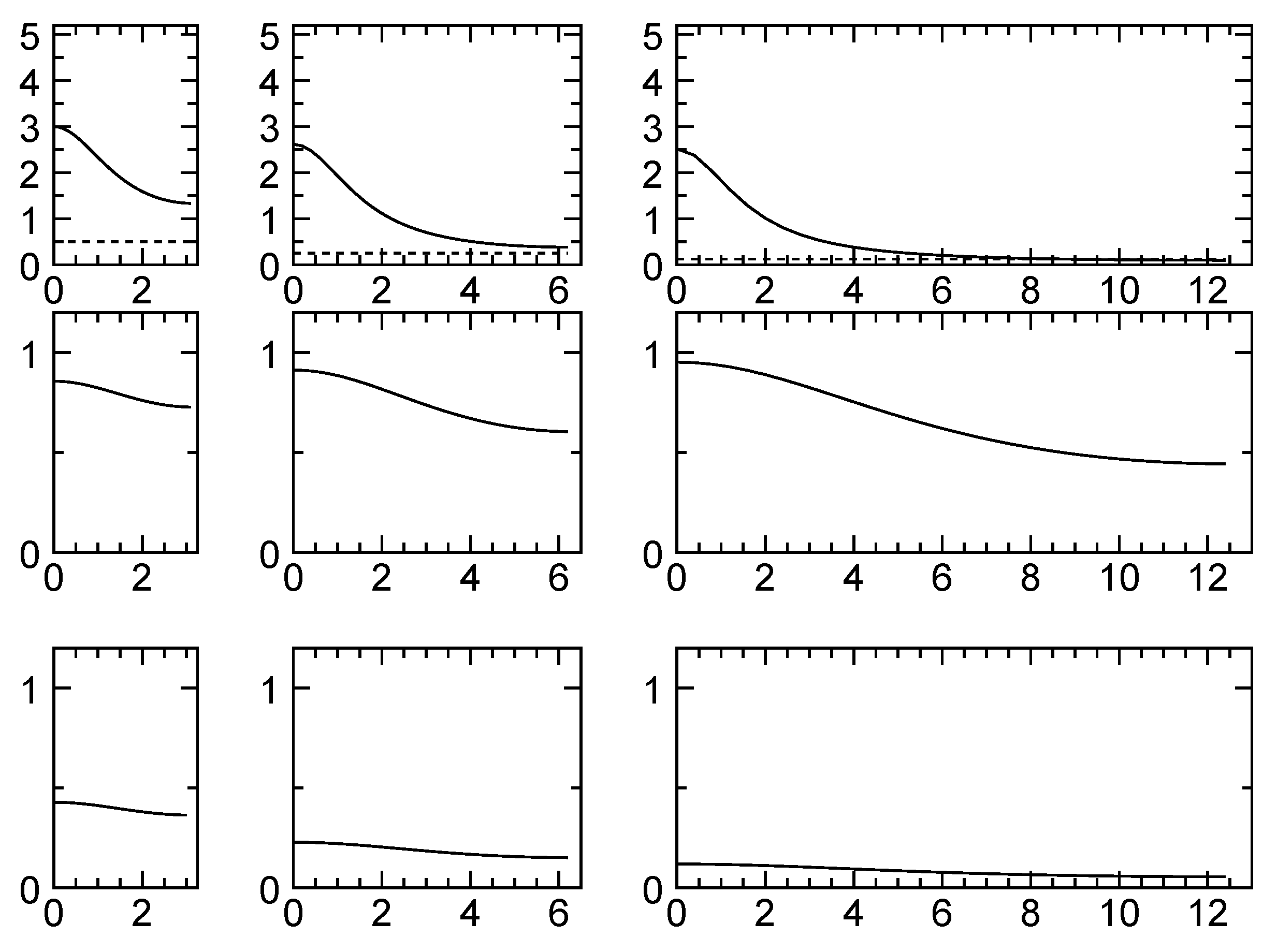
Figure 2: 

N_data < N_obs and increasing N_obs leads to essentiality no change in N_data. This shows the diminishing returns that are achieved in the case of correlated observations.

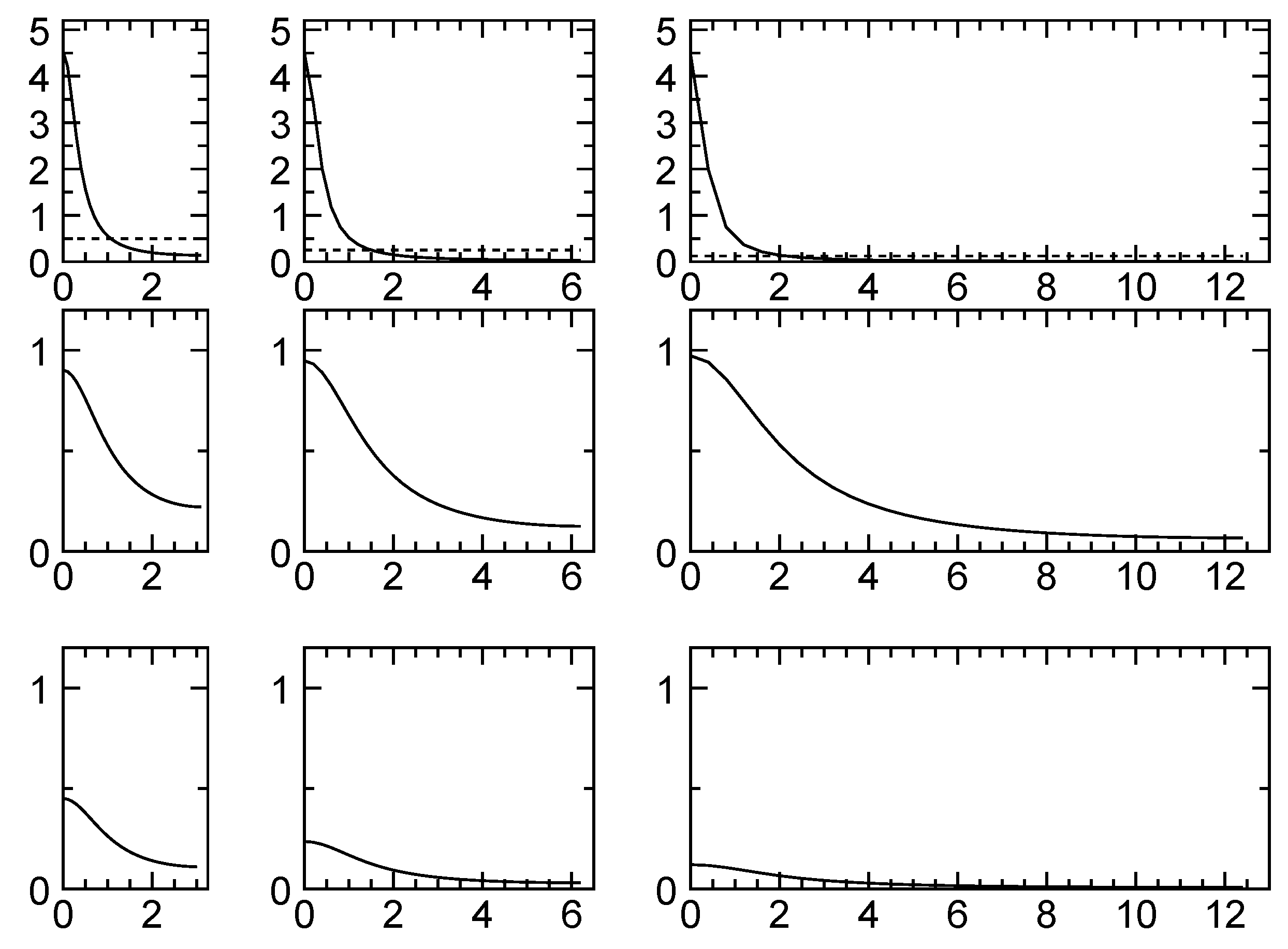
Figure 3: 

N_data < M_signal shows an analysis that is erroneous due to ignoring the role of truncation error. This gives a calculated value of the mean-square error that changes little with N_data.

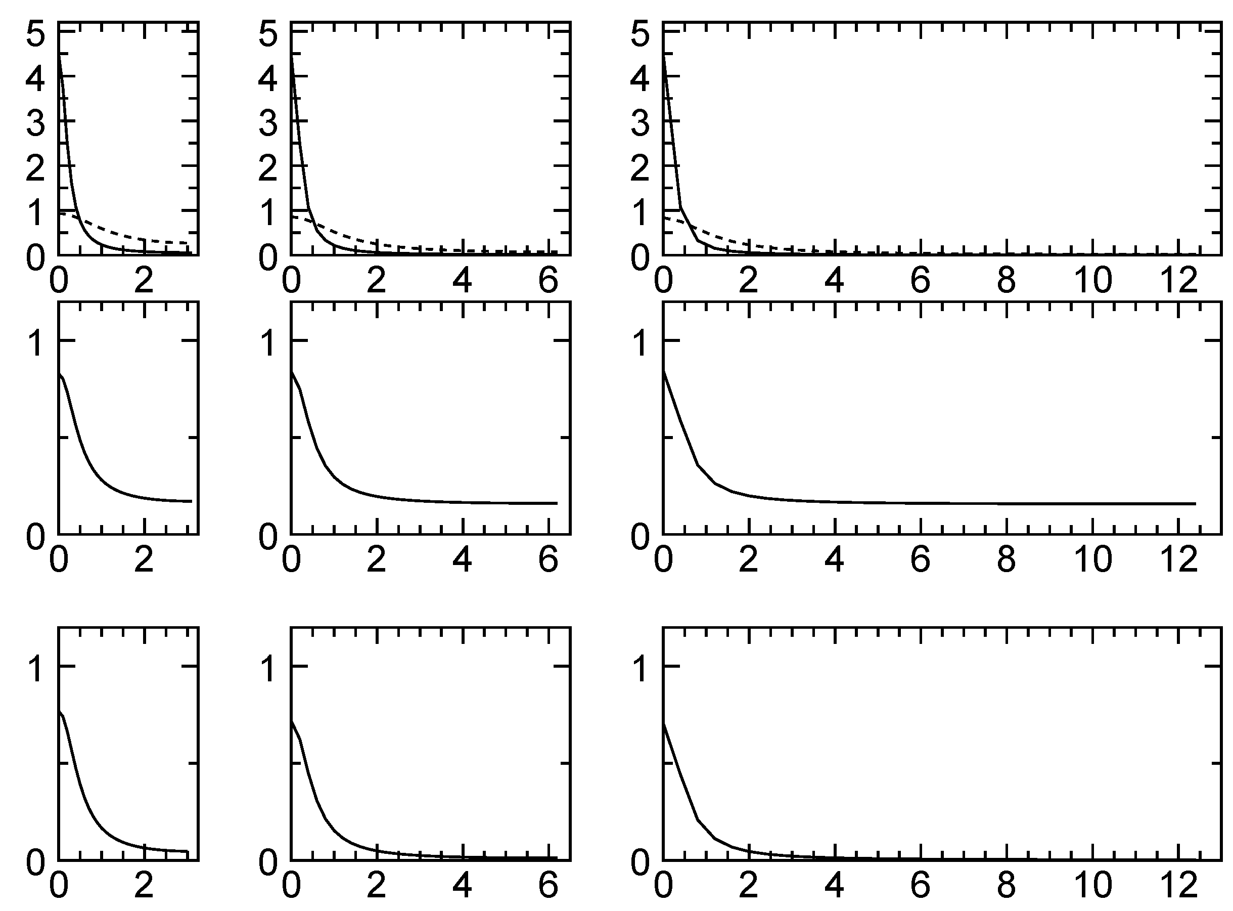
Figure 4: 

N_data < M_signal shows the same case as Figure 3 with signal aliasing now treated as a truncation error. Once this truncation error is accounted for, it can be seen that increasing N_obs reduces the mean-square-error due to reduction of truncation error.

The correction for truncation error as shown in Figure 4 is a very specific case of the general formalism described by Trampert and Sneider [22]. Applicability to the 2-D CO₂ inversion problem was demonstrated by Kaminski et al. [23].

For analysing non-stationarity time series, the Kalman filter formalism [24] considers a generic time series model which is a mixture of stochastic and deterministic components. The formalism is based on the simplest cases of each: linear relations for the deterministic component and Gaussian random variables for the stochastic components.

Figure 1. The effect of changing resolution on digital filtering. Going from left to right, the data spacing in successive columns decreases by a factor of 2 as $N_{\mathrm{data}}=N_{\mathrm{obs}}$ doubles and redoubles. For independent data the error spectrum $h_e\propto \Delta t$. Upper row shows $h_f(\omega )$ (solid) and $h_e(\omega )$ (dotted), middle row shows ${\Psi }_{\mathrm{OPT}}(\omega )$, the response of optimal filter, and bottom row shows the integrand of the mean-square error expression (12).

Figure 1. The effect of changing resolution on digital filtering. Going from left to right, the data spacing in successive columns decreases by a factor of 2 as $N_{\mathrm{data}}=N_{\mathrm{obs}}$ doubles and redoubles. For independent data the error spectrum $h_e\propto \Delta t$. Upper row shows $h_f(\omega )$ (solid) and $h_e(\omega )$ (dotted), middle row shows ${\Psi }_{\mathrm{OPT}}(\omega )$, the response of optimal filter, and bottom row shows the integrand of the mean-square error expression (12).

The Kalman filter formalism is an example of Bayes rule for sequential use of information. Although the equations are conventionally written in terms of changes, they are equivalent to Gaussian weighting of prediction and observation by inverse covariance matrices. The Kalman filter gives the optimal estimate of the model ‘state’ given a sequence of noisy measurements of linear projections of the state. More specifically it is the optimal one-sided (i.e. real-time) estimate. More precise estimates can be obtained if a lag is introduced between observation and estimation. The formalism for such estimation is known as the ‘Kalman smoother’ [24]. The model state can include model parameters, and so the Kalman filter can be used for calibration, although this will often require a generalisation to a non-linear formalism.

The deconvolution problem (solving Equation (6) for $S(t)$) can be expressed in the Kalman filter formalism. This has been done for CO₂ [19] (actually using the extended Kalman filter to deal with weak non-linearity in the processes). Estimation of model parameters uses a ‘model’ in which the ‘state’ is fixed, but the estimates of the state evolve as additional data is added. This leads to a simplification of the Kalman filter equations e.g. [5, Box 4.4].

One of the important advantages of the Kalman filter formalism is the ability to handle non-stationarity. However, it is often useful to consider how the tradeoff between prediction error and observation error behaves by considering the stationary case and using an analysis like that above to show the implications of different model formulations, e.g. Trudinger et al. [25].

Figure 2. The effect of changing resolution on digital filtering for the case of correlated errors. As in Figure 1, the data spacing in successive columns decreases by a factor of 2. Upper row shows $h_f(\omega )$ (solid) and $h_e(\omega )$ (dotted), middle row shows ${\Psi }_{\mathrm{OPT}}(\omega )$, the response of optimal filter, and bottom row shows the integrand of the mean-square error expression (12).

Figure 2. The effect of changing resolution on digital filtering for the case of correlated errors. As in Figure 1, the data spacing in successive columns decreases by a factor of 2. Upper row shows $h_f(\omega )$ (solid) and $h_e(\omega )$ (dotted), middle row shows ${\Psi }_{\mathrm{OPT}}(\omega )$, the response of optimal filter, and bottom row shows the integrand of the mean-square error expression (12).

4. A Carbon Cycle Analysis

4.1. A Model Space

The role of model error in an inverse problem is formally equivalent to that of data error (and a combined inverse covariance matrix can be obtained by combining inverse covariance matrices for model and data [1]). However, in a data space, model errors are likely to be highly correlated. While Abramowitz, [26] has proposed a ‘distance metric’ within a sample of models, this structure falls short of defining any sort of probability distribution.

As an example of how probabilities of models might be conceptualised, this section takes the relation between concentrations and emissions of CO₂, expressed as a response function in equation (6) and considers how this relation might be expressed in neighbouring parts of the modelling spectrum.

To consider the issue of ‘model error’ in a space of functions requires a representation of an appropriate class of function and a way of imposing the constraints $R(t)\ge 0$, and $\dot{R}(t)\le 0$ which reflect the dissipative nature of the system. Representing the response function by a discretisation in time is possible but even for deterministic calculations, the ill-conditioning leads to significant numerical difficulties [27,28]. Similar difficulty could be expected if using such a discretised form in the Kalman filter, which has the additional difficulty of being unable to apply the constraints $R(t)\ge 0$, and $\dot{R}(t)\le 0$ directly.

All these difficulties are magnified when one wants to consider a statistical distribution of functions while still preserving the constraints. As noted by Enting [29], the 20th century CO₂ record really only constrains a single moment of $R(t)$ and gives little additional information about the function.

Figure 3. The effect of changing resolution on digital filtering. The data spacing in successive columns decreases by a factor of 2. Upper row shows $h_f(\omega )$ (solid) and $h_e(\omega )$ (dotted), middle row shows ${\Psi }_{\mathrm{OPT}}(\omega )$, the response of optimal filter, and bottom row shows the integrand of the mean-square error expression (12).

Figure 3. The effect of changing resolution on digital filtering. The data spacing in successive columns decreases by a factor of 2. Upper row shows $h_f(\omega )$ (solid) and $h_e(\omega )$ (dotted), middle row shows ${\Psi }_{\mathrm{OPT}}(\omega )$, the response of optimal filter, and bottom row shows the integrand of the mean-square error expression (12).

As noted by Lindley [16] “...prior distributions, though usually anathema to the statistician, are essential to the notion of experimental information”. The present section proposes (with some preliminary analysis) a ‘maximum entropy’ approach to describing a prior distribution of $R(t)$. The first step is to note that all modelling is conditional (and thus probabilities are conditional). Indeed in climate modelling, calculations conditional on scenarios have been given the specific term ‘projections’. In scenario development, departures from ‘business-as-usual’ generally assume no asteroid impact, no pandemics, no thermonuclear war etc.

The ‘conditional’ aspect of the present approach is to confine a domain of interest in terms of time-scales on a range of about 5 years to 300 years. For computational practicality, discretised representations have to be used. $R(t)$ is represented as a discretised directed random-walk starting with $R(0)=1$, with discretisation, m, (with (6) modified to include a conversion from mass to concentration units). The maximum entropy approach would be to regard all candidate functions as equally likely, with no further constraints. However, the dicretisation process reveals that ‘equally likely’ can only be defined in terms of some specification of relative measures on t and $R(t)$. In the dicretised representation this translates into a need to specify relative probabilities of steps. At each annual time step, the change in $R(t)$ is either 0 or $-1/m$, subject to $R(t)\ge 0$. The prior probabilities of these steps were set at $1-m/300$ and $m/300$ respectively so that an ‘average’ walk would go to zero at $t=300$. Thus ‘equally likely’ is being defined in terms of the domain of interest.

The various data constraints are:

• CO₂ concentrations: the examples here use various combinations, from [30], of C(1990) = 353 ppm, C(1980) = 338 ppm, C(1970) = 325 ppm and C(1960) = 316 ppm.
  Figure 4. The effect of changing resolution on digital filtering. As for Figure 3 but with signal truncation treated as error. The data spacing in successive columns decreases by a factor of 2. Upper row shows $h_f(\omega )$ (solid) and $h_e(\omega )$ (dotted), middle row shows ${\Psi }_{\mathrm{OPT}}(\omega )$, the response of optimal filter, and bottom row shows the integrand of the mean-square error expression (12).

  Figure 4. The effect of changing resolution on digital filtering. As for Figure 3 but with signal truncation treated as error. The data spacing in successive columns decreases by a factor of 2. Upper row shows $h_f(\omega )$ (solid) and $h_e(\omega )$ (dotted), middle row shows ${\Psi }_{\mathrm{OPT}}(\omega )$, the response of optimal filter, and bottom row shows the integrand of the mean-square error expression (12).
• the pre-industrial concentration, C(t₀). In the examples given here, a fixed value of 280 ppm was used. A more comprehensive study should allow for uncertainty in this quantity.
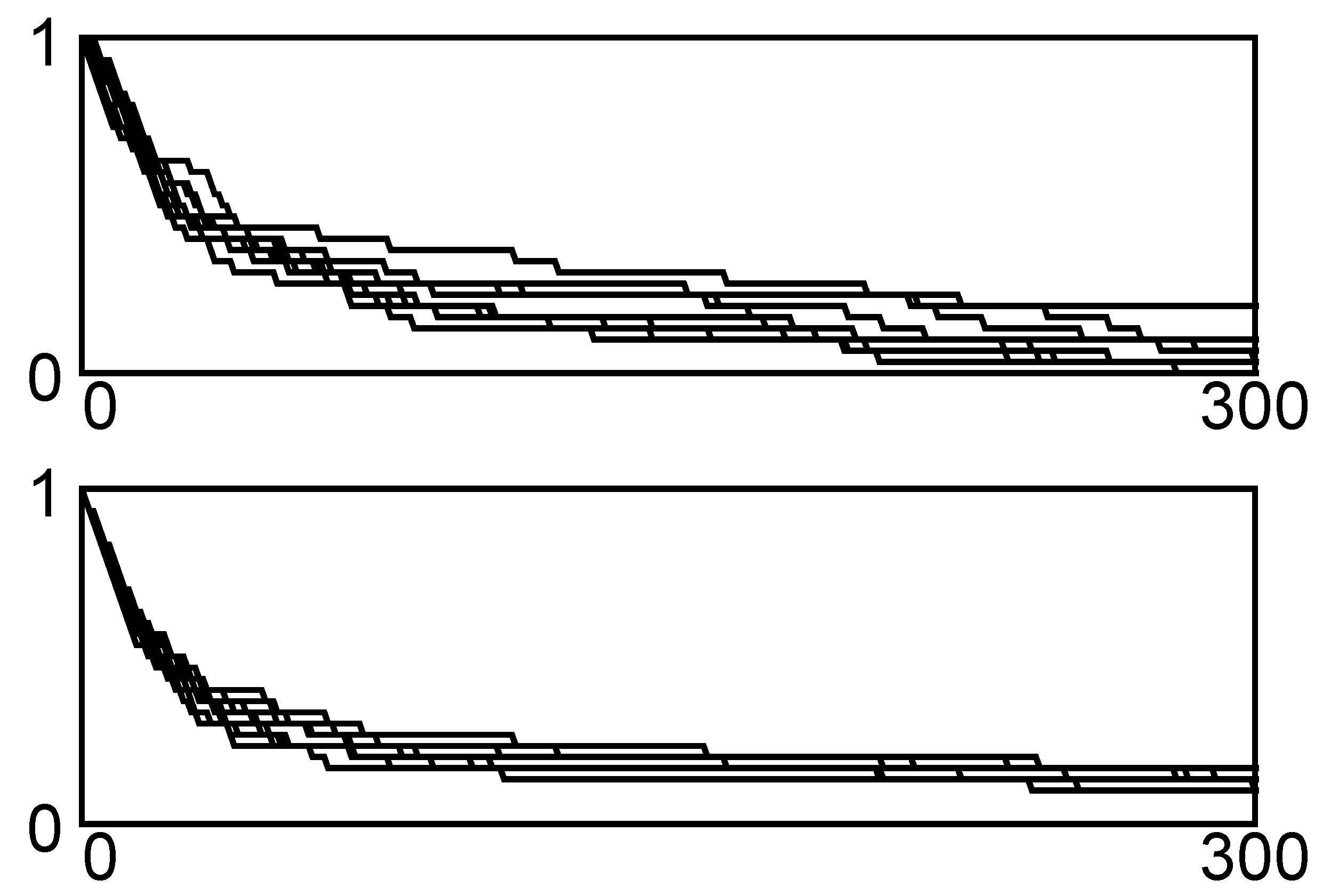
• A constraint on the value of R(300). A constraint of R(300) ≥ 0.1 was applied in some cases. The long-term behaviour of R(t) forms an important difference between ‘mainstream’ carbon cycle modelling and the various studies by Young and co-workers. The requirement that R(t) is of order 0.15 at long times follows from basic oceanic chemistry, combined with the requirements of conservation of mass
• A more comprehensive analysis would also consider uncertainties in the emissions, particularly those associated with changes in land use.
• Analogous linear programming studies, [27,28], suggest that a constraint R(t) ≥ 0 might also provide additional information, but this is not considered here.

Bayesian estimation was performed using a Markov Chain Monte Carlo (MCMC) approach to sample for the posterior distribution defined by the ‘maximum entropy’ prior and a likelihood obtained from relation (6) using observed CO₂ data. Each update step involved a potential change in the increment of $R(t)$ at a particular time step.

In order to analyse the extent to which the model behaviour was constrained outside its domain of definition, calculations were performed for $C(2100)$, firstly assuming a business-as-usual emission scenario (IS92a from the IPCC) and secondly assuming IS92a emissions to 2020 and then zero emissions thereafter.

The MCMC simulations produced candidate functions, $R(t)$, by successive updates of the walk direction at randomly chosen time steps. These were accepted according to probabilities based on the prior distribution of the walks and the likelihood of the calibration data, obtained by using the candidate $R(t)$ in (6). The observations were assumed to have normally distributed errors, with standard deviations as shown in Table 1 for various cases. In order to reduce the effect of correlations in the sampling, the results were sampled once every 200 update attempts.

As might be expected in a scoping study, various technical issues were identified. In particular the choice of discretisation, m, represented a compromise. With m too large, the representation of $R(t)$ could not capture an initial decline (this could potentially be avoided by allowing a range of step sizes). With m too small, the sampling tended to get ‘stuck’ in low-probability regions near the boundary defined by $R(t)\ge 0$ (this could potentially be avoided with a more sophisticated update strategy). In general, it is expected that adopting techniques from lattice statistical mechanics will provide algorithmic refinements to the scoping study presented here.

In terms of the information measures defined above, the Monte Carlo technique is best suited to measures such as the Kullback-Leibler divergence that evaluate information relative to the posterior distribution. However, given the preliminary nature of the present study, distributions have simply been compared in terms of standard deviations for the distributions of various quantities.

4.2. Results

As has been noted before, the analysis of the information content of fitting response functions is illustrative and does not reflect the current state of knowledge of the carbon cycle. Most notably no ¹⁴C data have been used. The actual history of carbon cycle modelling reveals that the major reservoirs and turnover times had been identified [31, for example], prior to the availability of ice-core data that gave pre-1958 CO₂ concentrations. While the CO₂ concentration record has played only a part of the development of current understanding, it provides a convenient case of analysing one example of information content.

The ‘maximum entropy’ analyses were performed for a range of cases, with some representative results shown in Table 1. These cases have $R(t)$ discretised in increments of $1/30$. The results for discretisation at increments of $1/20$ are found to be generally similar. Figure 5 shows superpositions of 10 samples of $R(t)$ for cases 2 and 5 of Table 1.

The column $C(2100)$ with IS92a represents a business-as-usual case, i.e. no major departures from exponential growth. As such, an adequate approximation can be expected from a black-box representations (constant airborne fraction approximation) [29]. Thus for, the relevant aspect of the information in the data is how much it contributes to reducing uncertainties in this one moment of $R(t)$.

The column $C(2100)$ with $S(t>2020)=0$ is an exaggerated form of the reductions that will be required in order to stabilise atmospheric CO₂. The behaviour depends on multiple time-scales that are poorly represented by direct calibration. This can be seen by the fact that the absolute uncertainties are comparable to those of the ‘business-as-usual’ case, even though much smaller emissions are involved.

Before these results can be regarded as representing a measure of the real carbon cycle uncertainty implied by CO₂ data, various limitations alluded to above must be removed. The most important of these are:

Table 1. Results of Bayesian fit of response functions, using ‘directed random walk’ distribution for prior. The response function $R(t)$ is discretised into $m+1$ levels from 1 to 0, with some cases subject to having $R(t)\ge R_{\min }$ and fitted to concentration data for the times specified in the ‘Times’ column. Calculated concentrations, $C(t)$, are listed for 3 cases and are given in ppm.

Case	m	$R_{\min }$	Times	Range	$C(1990)$	$C(2100)$	$C(2100)$
						IS92a	$S(t>2020)=0$
1	30	0.1	1960	$\pm 2$ ppm	$366.1\pm 2.4$	$683.7\pm 16.1$	$352.1\pm 10.9$
2	30	0.0	1960	$\pm 2$ ppm	$365.9\pm 2.4$	$636.1\pm 17.4$	$338.9\pm 12.9$
3	30	0.1	1990	$\pm 2$ ppm	$357.2\pm 3.2$	$582.9\pm 11.9$	$323.4\pm 12.5$
4	30	0.0	1990	$\pm 2$ ppm	$353.0\pm 1.2$	$575.5\pm 12.0$	$319.8\pm 10.3$
5	30	0.1	1960,70,80,90	$\pm 4$ ppm	$357.4\pm 1.5$	$600.4\pm 11.4$	$336.9\pm 9.2$
6	30	0.0	1960,70,80,90	$\pm 4$ ppm	$357.4\pm 1.6$	$590.1\pm 14.0$	$325.1\pm 11.9$

Table 1. Results of Bayesian fit of response functions, using ‘directed random walk’ distribution for prior. The response function $R(t)$ is discretised into $m+1$ levels from 1 to 0, with some cases subject to having $R(t)\ge R_{\min }$ and fitted to concentration data for the times specified in the ‘Times’ column. Calculated concentrations, $C(t)$, are listed for 3 cases and are given in ppm.

Case	m	$R_{\min }$	Times	Range	$C(1990)$	$C(2100)$	$C(2100)$
						IS92a	$S(t>2020)=0$
1	30	0.1	1960	$\pm 2$ ppm	$366.1\pm 2.4$	$683.7\pm 16.1$	$352.1\pm 10.9$
2	30	0.0	1960	$\pm 2$ ppm	$365.9\pm 2.4$	$636.1\pm 17.4$	$338.9\pm 12.9$
3	30	0.1	1990	$\pm 2$ ppm	$357.2\pm 3.2$	$582.9\pm 11.9$	$323.4\pm 12.5$
4	30	0.0	1990	$\pm 2$ ppm	$353.0\pm 1.2$	$575.5\pm 12.0$	$319.8\pm 10.3$
5	30	0.1	1960,70,80,90	$\pm 4$ ppm	$357.4\pm 1.5$	$600.4\pm 11.4$	$336.9\pm 9.2$
6	30	0.0	1960,70,80,90	$\pm 4$ ppm	$357.4\pm 1.6$	$590.1\pm 14.0$	$325.1\pm 11.9$

• treat the notional pre-industrial equilibrium concentration as an uncertain quantity;
• consider the uncertainties in the emissions, S(t), over the calibration period — this is particularly important for emissions from land-use change.

As increasing amounts of data are used, more careful statistical modelling of the data error, addressing issues described in [4], will be needed

Such refinements are essential before the present methodology could provide a basis to answer question: how much of the information in posterior distribution (i.e. the calibrated model) is coming from assumed model structure? and how much represents actual observations? In other words, do the additional constraints implied by parametric statistical fits or lumped model representation significantly change the information content of models?

4.3. Extensions

In discussing how the analysis in this paper might be extended, two different aspects need to be distinguished:

• firstly, there is the extension of the analysis of the global-scale behaviour. This includes both a comprehensive exploration of the ideas outlined in the previous section and the incorporation of additional available data, most notably ¹⁴C data;
• secondly there is the extension of carbon cycle modelling to become part of more comprehensive earth system modelling.

The restriction to using only atmospheric CO₂ data in the analysis above comes from the requirement of simplicity of presentation. As noted above, this departs from the historical ordering where ¹⁴C data provide much of the information about the carbon cycle at a time when the direct (post-1958) observation record was short, and ice-core data were not available [31]. The traditional approach to using ¹⁴C data has been to use models from the more deterministic end of the spectrum. However a joint representation in terms of related response functions for CO₂ and ¹⁴CO₂ was described by Enting [32]. This could provide a basis for moving ¹⁴C analysis further towards the ‘black-box end of the spectrum in order to quantify the information, but this is beyond the scope of the present paper. In addition to the ¹⁴C data, other observations that can constrain uncertainties about the global carbon cycle include ¹³C data, atmospheric O₂:N₂ trends and measurements of oceanic uptake of tritium (from nuclear testing) and CFCs.

Figure 5. Samples of response functions $R(t)$ constrained only by CO₂ data, superimposing 10 realisations from the Markov Chain Monte Carlo calculations. Cases 2 (upper) and 5 (lower) from Table 1.

Figure 5. Samples of response functions $R(t)$ constrained only by CO₂ data, superimposing 10 realisations from the Markov Chain Monte Carlo calculations. Cases 2 (upper) and 5 (lower) from Table 1.

There are many reasons for incorporating the carbon cycle into a fully-interactive earth system model. One of the most important of these is the possibility of climate-to-carbon feedbacks occurring over the 21st century. The IPCC 4th Assessment report [33] regards the extent of such processes as being one of the two greatest unknowns in the medium-term evolution of climate — ice-sheet instability being the other.

An important, and poorly-understood part of potential climate-to-carbon feedback comes from the land surface. Efforts to improve understanding have focused on the development of improved land-surface modelling in climate models. The aim is to have process-based models represent the fluxes of carbon and water between land and atmosphere (and represent the coupling between these fluxes). The term ‘multiple constraints’ [34, for example] has been used in recognition of the fact such development will need to draw on a diversity of data streams. The author’s involvement in development of land surface modelling in ACCESS (Australian Community Climate and Earth System Simulator) is the motivation for the present study.

Some of the main data sources for such model development have been described by Canadell et al. [35] as:

• Air sampling networks interpreted by inverse modelling;
• Satellite data, for quantities such as leaf-area index and phenology
• Terrestrial biosphere models;
• Convective boundary layer measurements;
• Stand-level flux networks;
• Ecosystem experiments;
• Small cuvettes.

The statistical issues that need to be addressed when using such multiple data streams have been characterised (in qualitative terms) by Raupach et al. [36] as:

• magnitude;
• degree of correlation between components;
• temporal correlation structure;
• spatial correlation structure;
• distribution;
• mismatches in averaging;
• contribution from model representativeness error.

A study by Abramowitz [37] found that the predictive power of empirical models (statistical fits implemented by an artificial neural network) was better than that achieved by process-based land-surface models when predicting fluxes, given meteorological forcing. It is to be hoped that the techniques described in the previous section can clarify the nature of that result.

5. Concluding Remarks

As emphasised in Section 4, the analysis of uncertainties in the carbon cycle must be regarded as illustrative since no ¹⁴C data have been considered in the analysis here. In reality, uncertainties in the behaviour of the carbon cycle over decadal scales are dominated by the correlated uncertainties in the emissions from land-use change and the processes of the so-called CO₂-fertilisation [38].

The ‘maximum entropy’ calculations using a directed random walk discretisation of a response function should be regarded as a proof of concept. The ‘directed random walk’ prior model for $R(t)$ is comparable to the use of random walks as the prior distribution forcings such as $S(t)$. This approach gives a computationally-feasible way of representing uncertainties in response functions in a non-parametric form, as recommended by Evans and Stark [20], that is sufficiently general to encompass both parametric statistical fits and fits based on lumped model representations. The ability to treat multiple approaches on an even footing provides the basis for studying the extent to which various modelling approaches are imposing constraints beyond those implied by actual observational data.

References and Notes

- Tarantola, A. Inverse Problem Theory: Methods for Data Fitting and Model Parameter Estimation; Elsevier: Amsterdam, 1987. [Google Scholar]
- Young, P.; Garnier, H. Identification and estimation of continuous-time data-based mechanistic models for environmental systems. Environmen. Modell. Softw. 2006, 21, 1055–1072. [Google Scholar]
- Karplus, W. J. The spectrum of mathematical modelling and systems simulation. Math. Comput. Simul. 1977, 19, 3–10. [Google Scholar]
- Enting, I. G. Characterising the temporal variability of the global carbon cycle; CSIRO Atmospheric Research Technical Paper no. 40; CSIRO: Australia, 2000; http://www.dar.csiro.au/publications/enting 2000a.pdf.
- Enting, I. G. Inverse Problems in Atmospheric Constituent Transport; CUP: Cambridge, UK, 2002. [Google Scholar]
- Enting, I. G.; Wigley, T. M. L.; Heimann, M. Future emissions and concentrations of carbon dioxide: Key/ocean/atmosphere/land analyses; CSIRO Division of Atmospheric Research Technical Paper no. 31; CSIRO: Australia, 1994; http://www.dar.csiro.au/publications/enting 2001a.htm.
- Enting, I. G. Twisted: The Distorted Mathematics of Greenhouse Denial; I. Enting/Australian Mathematical Sciences Insititute: Melbourne, 2007. [Google Scholar]
- Christie, M. The Ozone Layer: A Philosophy of Science Perspective; CUP: Cambridge, U.K., 2000. [Google Scholar]
- Kellogg, W. W. Effects of Human Activities on Global Climate; Technical Note 156; WMO: Geneva, 1977. [Google Scholar]
- Gwynne, P. The cooling world. Newsweek 1975, 28 April 1975, 64. [Google Scholar]
- Young, P.; Parkinson, S.; Lees, M. Simplicity out of complexity in environmental modelling: Occam’s razor revisited. J. Appl. Statist. 1996, 23, 165–210. [Google Scholar] [CrossRef]
- Enting, I. G. A modelling spectrum for carbon cycle studies. Math. Comput. Simul. 1987, 29, 75–85. [Google Scholar] [CrossRef]
- Rayner, P. J.; Enting, I. G.; Trudinger, C. M. Optimizing the CO2 observing network for constraining sources and sinks. Tellus 1996, 48B, 433–444. [Google Scholar] [CrossRef]
- Rayner, P. J.; O’Brien, D. The utility of remotely sensed CO2 concentration data in surface source inversions. Geophys. Res. Lett. 2001, 28, 175–178. [Google Scholar] [CrossRef]
- Shannon, C. E. A mathematical theory of communication. Bell Sys. Tech. J. 1948, 27, 379–423, 623–565. [Google Scholar] [CrossRef]
- Lindley, D. V. On a measure of the information provided by an experiment. Ann. Math. Statist. 1956, 27, 986–1005. [Google Scholar] [CrossRef]
- Kullback, S.; Leibler, R. A. Information and sufficiency. Ann. Math. Statist. 1951, 22, 79–86. [Google Scholar] [CrossRef]
- Oeschger, H.; Heimann, M. Uncertainties of predictions of future atmospheric CO2 concentrations. J. Geophys. Res. 1983, 88C, 1258–1262. [Google Scholar] [CrossRef]
- Trudinger, C. M.; Enting, I. G.; Rayner, P. J.; Francey, R. J. Kalman filter analysis of ice core data. 2 Double deconvolution of CO2 and δ13C measurements. J. Geophys. Res. 2002, 107. [Google Scholar]
- Evans, S. N.; Stark, P. B. Inverse problems as statistics. Inverse Prob. 2002, 18, R55–R97. [Google Scholar] [CrossRef]
- Wunsch, C.; Minster, J.-F. Methods for box models and ocean circulation tracers: Mathematical programming and non-linear inverse theory. J. Geophys. Res. 1982, 87C, 5647–5662. [Google Scholar]
- Trampert, J.; Sneider, R. Model estimation biased by truncated expansions: Possible artifacts in seismic tomography. Science 1996, 271, 1257–1260. [Google Scholar] [CrossRef]
- Kaminski, T.; Rayner, P. J.; Heimann, M.; Enting, I. G. On aggregation errors in atmospheric transport inversions. J. Geophys. Res. 2001, 106, 4703–4715. [Google Scholar] [CrossRef]
- Gelb, A. (Ed.) Applied Optimal Estimation; MIT Press: Cambridge, Mass, 1974.
- Trudinger, C. M.; Raupach, M. R.; Rayner, P. J.; Enting, I. G. Using the Kalman filter for parameter estimation in biogeochemical models. Environmetrics 2008, (in press). [Google Scholar] [CrossRef]
- Abramowitz, G.; Gupta, H. Towards a model space and independence metric. Geophys. Res. Lett. 2008, 35, L05705. [Google Scholar] [CrossRef]
- Enting, I. G.; Mansbridge, J. V. The incompatibility of ice-core CO2 data with reconstructions of biotic CO2 sources. Tellus 1987, 39B, 318–325. [Google Scholar] [CrossRef]
- Enting, I. G. The incompatibility of ice-core CO2 data with reconstructions of biotic CO2 sources (II). The influence of CO2-fertilised growth. Tellus 1992, 44B, 23–32. [Google Scholar] [CrossRef]
- Enting, I. G. Laplace transform analysis of the carbon cycle. Environ. Modell. Softw. 2007, 22, 1488–1497. [Google Scholar] [CrossRef]
- Keeling, C. D.; Whorf, T. P. Atmospheric records from the SIO sampling network. In Trends ’93: A Compendium of Data on Global Change; Boden, T. A., Kaiser, D. P., Serpinski, R. J., Stoss, F. W., Eds.; CDIAC, ORNL: Oak Ridge, 1994. [Google Scholar]
- Broecker, W. S.; Peng, T.-H.; Engh, R. Modeling the carbon system. Radiocarbon 1980, 22, 565–598. [Google Scholar]
- Enting, I. G. Ambiguities in the calibration of carbon cycle models. Inverse Prob. 1990, 6, L39–L46. [Google Scholar] [CrossRef]
- Alley, R.; et al. Summary for Policymakers. In Climate Change 2007, The Physical Basis; Solomon, S., Qin, D., Manning, M., Chen, Z., Marquis, M., Avery, K., Tignor, M., Miller, H., Eds.; Published for the IPCC by CUP: Cambridge, UK, 2007. [Google Scholar]
- Kruijt, B.; Dolman, A. J.; Lloyd, J.; Ehleringer, J.; Raupach, M.; Finnigan, J. Assessing the regional carbon balance: Towards an integrated, multiple constraints approach. Change 2001, 56 (March– April 2001), 9–12. [Google Scholar]
- Canadell, J. G.; et al. Carbon metabolism of the terrestrial biosphere: A multitechnique approach for improved understanding. Ecosystems 2000, 3, 115–130. [Google Scholar] [CrossRef]
- Raupach, M. R.; Rayner, P. J.; Barrett, D. J.; DeFries, R. S.; Heimann, M.; Ojima, D. S.; Quegan, S.; Schmullius, C. C. Model-data synthesis in terrestrial carbon observation: methods, data requirements and data uncertainty specifications. Glob. Change Biol. 2005, 11, 378–397. [Google Scholar] [CrossRef]
- Abramowitz, G. Towards a benchmark for land surface models. Geophys. Res. Lett. 2005, 32, L22702. [Google Scholar] [CrossRef]
- Enting, I. G.; Lassey, K. R. Projections of future CO2; CSIRO Division of Atmospheric Research Technical Paper no. 27; CSIRO: Australia, 1993; http://www.dar.csiro.au/publications/enting 2000e.pdf.
© 2008 by the authors; licensee MDPI, Basel, Switzerland. This article is an open access article distributed under the terms and conditions of the Creative Commons Attribution license (http://creativecommons.org/licenses/by/3.0/).
Share and Cite
Enting, I.G. Assessing the Information Content in Environmental Modelling: A Carbon Cycle Perspective. Entropy 2008, 10, 556-575. https://doi.org/10.3390/e10040556
Enting IG. Assessing the Information Content in Environmental Modelling: A Carbon Cycle Perspective. Entropy. 2008; 10(4):556-575. https://doi.org/10.3390/e10040556
Chicago/Turabian StyleEnting, Ian G. 2008. "Assessing the Information Content in Environmental Modelling: A Carbon Cycle Perspective" Entropy 10, no. 4: 556-575. https://doi.org/10.3390/e10040556
APA StyleEnting, I. G. (2008). Assessing the Information Content in Environmental Modelling: A Carbon Cycle Perspective. Entropy, 10(4), 556-575. https://doi.org/10.3390/e10040556