The Entropy Principle from Continuum Mechanics to Hyperbolic Systems of Balance Laws: The Modern Theory of Extended Thermodynamics

Abstract

We discuss the different roles of the entropy principle in modern thermodynamics. We start with the approach of rational thermodynamics in which the entropy principle becomes a selection rule for physical constitutive equations. Then we discuss the entropy principle for selecting admissible discontinuous weak solutions and to symmetrize general systems of hyperbolic balance laws. A particular attention is given on the local and global well-posedness of the relative Cauchy problem for smooth solutions. Examples are given in the case of extended thermodynamics for rarefied gases and in the case of a multi-temperature mixture of fluids.

1. Entropy principle in continuum mechanics

The concept and name of entropy originated in the early 1850’s in the work of Rudolf Julius Emanuel Clausius (1822-1888):

”Heat cannot pass by itself from a cold to a hot body”.

In the classical approach of thermodynamics (the theory of non-equilibrium processes), the entropy principle characterizes the irreversibility of the processes, i.e. an arrow in the time direction. A different important point of view was proposed in the 60’ in the context of rational thermodynamics. To explain this different point of view it is necessary to recall the structure of continuum theories.

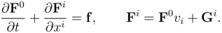
The physical laws in continuum theories are balance laws:

Let F⁰ (x, t) a generic density; x ∈ Ω, t ∈ R⁺. The time derivative in the domain Ω is expressed by

where the first integral on the r.h.s. represents the flux of some quantities Gⁱ through the surface Σ of unit normal n ≡ (n_i) and velocity v ≡ (v_i), while the last integral represents the productions.

Under regularity assumptions the system can be written in the local form:

For example in the case of fluids:

where ρ, v ≡ (v_i), t ≡ (t_ij), q ≡ (q_i), ε are respectively the mass density, the velocity, the stress tensor, the heat flux and the internal energy.

Of course the balance law systems are not closed, having more unknowns variables than equations and in order to close the system we need to introduce the so called constitutive equations . In the modern constitutive theory all the constitutive equations must obey the two principles:

• The objectivity principle: the constitutive equations are independent of the observer;
• the second principle of thermodynamics that in the Rational Thermodynamics requires that any solutions of the full system satisfies the Clausius-Duhem inequality (Coleman-Noll [1]) :

  (1)

with T denoting the absolute temperature and S the entropy density given by a constitutive relation to be determined by the compatibility between the balance Eqs. and (1). The requirement that all the solutions of the balance laws system satisfies also the new balance law (1) is so strong that several restrictions arise for admissible constitutive equations. For instance in the case of a classical approach for the fluids with Fourier Navier-Stokes assumptions

the constitutive equations compatible with Eq. (1) must satisfy:

(2)

and moreover

χ , µ , ν ≥ 0,

with t = −pI + σ, p is the pressure, σ is the shear stress, < ij > denotes the deviatoric part of a tensor, χ the heat conductivity, µ the shear viscosity and ν the bulk viscosity.

We observe that, with this new approach, the Gibbs relation (2) that gives a differential link between S, p, ε and ρ comes as a consequence of the entropy principle and is not assumed a priori as in the thermodynamics of irreversible process (TIP) (local equilibrium assumption). Introducing the free energy ψ = ε − TS, we deduce from (2) the well know conditions

that permit to obtain p, S and ε from the knowledge of a single function ψ ≡ ψ(ρ,T).

In the modern rational thermodynamics the entropy principle becomes a constraint for the acceptable constitutive equations.

The entropy principle is also supported by the kinetic theory of gases. The kinetic theory describes the state of a rarefied gas through the phase density f (x, t, c), where f (x, t, c)dc is the density of atoms at point x and time t that have velocities between c ≡ (c_i) and c + dc. The phase density obeys the Boltzmann equation

(3)

where Q represents the collisional terms. In fact from the Boltzmann equation introducing as moments:

(k is the Boltzmann constant) we have the so called H-theorem:

(4)

but the entropy flux φ_i is in general different from q_i/T.

The necessity to extend the entropy principle with a general entropy flux was proposed by I. Müller [2]. At the present the general form (4) is universally accepted in the continuum mechanics community and all the constitutive equations in new models are tested by the entropy principle.

2. The Riemann problem

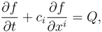
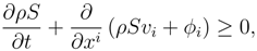
In a complete different context the entropy principle plays a fundamental role. The Riemann problem was originated by the well known problem of fluid-dynamics in which the fluid is initially maintained in two different equilibrium states separated by a membrane. This problem was generalized in the one-dimensional case for a general hyperbolic system of conservation laws assuming discontinuous constant initial data. It is well known that weak solutions are not unique for hyperbolic systems of conservation laws. The Riemann problem for an initial sufficiently small jump is solved as a ”superposition” of

Figure 1. (a) The Riemann initial data and (b) the Riemann with structure data.

Figure 1. (a) The Riemann initial data and (b) the Riemann with structure data.

shocks, characteristic shocks, rarefaction waves and constant states [3]. For genuine non linear waves (∇λ · r ≠ 0), the admissible physical shocks are those for which the Lax conditions hold

λ(u₀) < s < λ(u₁)

that are equivalent to the condition that the entropy production growth across the shock

η > 0.

For exceptional waves (linearly degenerate ∇λ · r ≡ 0) we have characteristic shocks:

λ(u₀) = s = λ(u₁)  ⇔ η = 0.

While if λ(u₁) < λ(u₀) we have a rarefaction wave. The λ’s denoting the characteristic velocities of the hyperbolic system, r being the corresponding right eigenvectors, ∇ = ∂/∂u, u₀ and u₁ being the constant initial data for the field u (as sketched in Figure 1a), s and η representing the shock velocity and the entropy production across the shock.

The problem fails in the special case of local exceptionality ∇λ · r = 0 for some u. In this case the stability of the shock must satisfy the Liu conditions [4], [5] that implies the generalized Lax condition λ(u₀) ≤ s ≤ λ(u₁) but the entropy growth alone is not sufficient for the admissibility. In fact it is necessary to add a new superposition principle for the shocks (Liu and Ruggeri [6]).

Therefore the entropy principle becomes a selection rule for constitutive equations for classical solutions and a selection rule for physical processes for weak solutions.

The Riemann problem is a fundamental tool for existence theorems but also is very important for the so called Riemann problem with structure, i. e. when the initial data are smooth functions connecting at ±∞ two different constant states (u₀, u₁) (see Figure 1b).

In fact there are the following asymptotic results due to Liu [4, 5]: For large time the solutions of the Riemann with structure problem converge to the corresponding solutions of the Riemann problem with discontinuous initial data (u₀, u₁) for genuine non-linear characteristic velocities, while for linearly degenerate characteristic velocity the corresponding wave tend to a traveling wave.

In particular, if the initial data are perturbations of a constant state (u₀ = u₁), then for large t the solution u converges to the constant state.

3. Dissipative hyperbolic systems

The entropy principle for hyperbolic systems plays an important role not only in the subject of the uniqueness of weak solutions:

• The systems endowed with an entropy principle with a convex entropy density can be written as a symmetric system if we choose a privileged field variables ”the main field” and the local Cauchy problem is well-posed;
• The main field induced the possibility to find nesting theories trough the definition of principal subsystem. In particular there exists an equilibrium manifold in which the entropy reaches the maximum value;
• If the hyperbolic system of balance laws has a dissipative character in the sense of Kawashima and Shizuta, there exist global smooth solutions and the equilibrium manifold is attractive provided the initial data are sufficiently small.

Let us consider a generic hyperbolic system of balance laws in a three dimensional space endowed with an entropy law. Using the compact space-time notation (α = 0, 1, 2, 3; x⁰ = t), we write the governing system and the entropy law in the form:

∂_αF^α(u) = f (u)

(5)

∂_αh^α(u) = Σ (u) ≤ 0,

(6)

where except for the sign h⁰, hⁱ and Σ have the meaning of entropy density, entropy flux and entropy production (see (4). The compatibility between (5) and (6) implies the existence of a main field u′ ≡ u′(u) such that:

∂_αh^α − Σ ≡ u′ · (∂_αF^α − f ) .

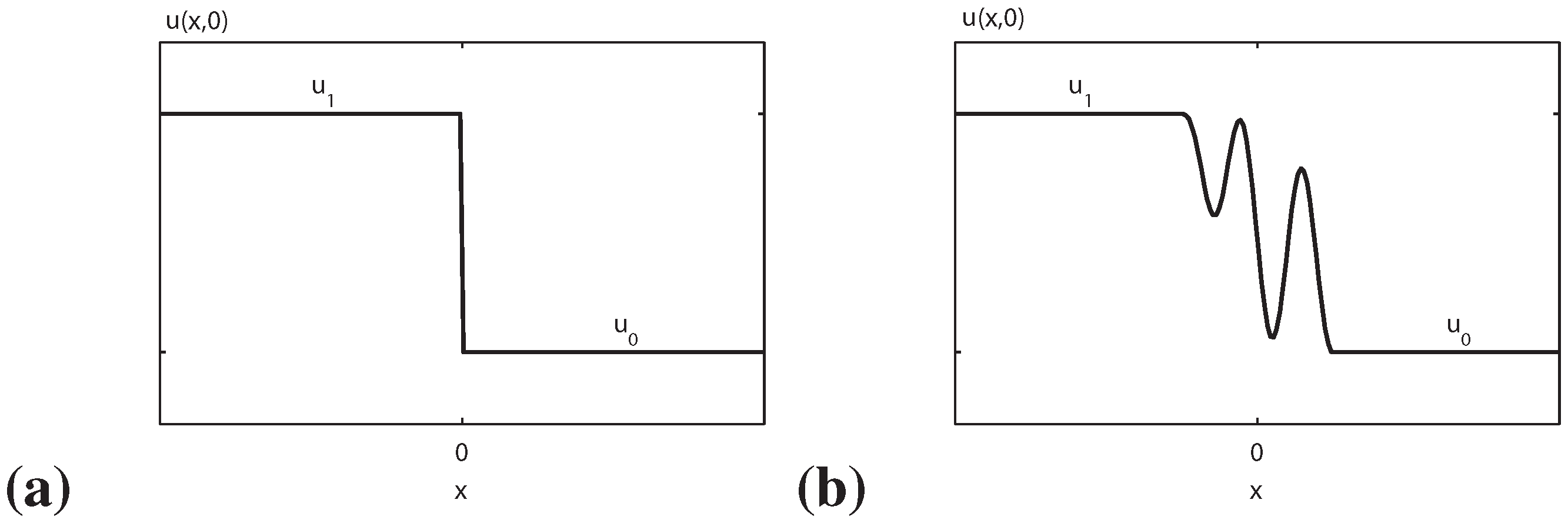
As a consequence of the above identity, we have

dh^α = u′ · dF^α, Σ = u′ · f ≤ 0.

(7)

It is possible to show (Boillat [7, 8], Ruggeri and Strumia [9]) that, because of (7)₁, there exist four potentials h′^α:

h′^α = u′ · F^α − h^α,

such that

It follows that, upon selecting the main field as the field variables, the original system (5) can be written with Hessian matrices in a (special) symmetric form

(8)

provided that h⁰ is a convex function of u ≡ F⁰ (or equivalently the Legendre transform h′⁰ is a convex function of the dual field u′.

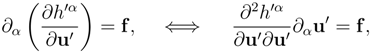
We split the main field u′ ∈ R^N in two parts u′ ≡ (v′, w′), where v′ ∈ R^M , and w′ ∈ R^N−M , (0 < M < N ). The system (8) with f ≡ (q, g)^T , reads:

(9)

Given some assigned constant value of w′, we call principal subsystem of (9) the system [10]:

The solutions of a principal subsystem satisfy a supplementary law (subentropy law):

where the entropy four-vector and the entropy production are related to the restrictions of the entropy four-vector h_α(v′, ) and of the entropy production Σ(v′, ) of the full system. The subentropy is convex and therefore every principal subsystem is symmetric hyperbolic.

Let respectively and the characteristic velocities of the total system and of the subsystem. In general the solutions of the subsystem are not particular solutions of the system (for w′ = ) and the spectrum of the is not part of the spectrum of the λ’s. However define

and similarly for the minima. Then, under the assumption that h⁰ is a convex function, the following subcharacteristic conditions hold for every principal subsystem:

(10)

(11)

∀ v′ ∈ R_M and

An interesting case is when the first M equations are conservation laws, i.e. when (9) reduce

(12)

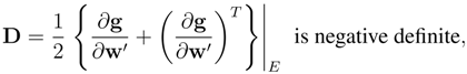
As usual in thermodynamics, we define the equilibrium state:

-An equilibrium state is a state for which the entropy production −Σ|_E vanishes and correspond to its minimal value.

In an equilibrium state, under the assumption of dissipative productions i.e. if

the production vanishes and the main field components vanish except for the first M ones (E stands for the equilibrium state). Thus

g|_E = 0, w′|_E = 0.

In this case

become the equilibrium sub-system of the system (12).

Moreover it is possible to prove that at equilibrium the entropy density −h is maximal, i.e.

h > h|_E ∀ u ≠ u|_E,    where   h|_E = h (v,w|_E (v)) .

4. Qualitative analysis

In the general theory of hyperbolic conservation laws and hyperbolic-parabolic conservation laws, the existence of a strictly convex entropy function, which is a generalization of the physical entropy, is a basic condition for the well-posedness ( Friedrichs and Lax [11], Kawashima [12]).

In fact, choosing u ≡ F₀ if the fluxes Fⁱ and the production f are smooth enough in a suitable convex open set D ∈ Rⁿ, it is well known that problem (5) has a unique local (in time) smooth solution for smooth initial data.

However, in the general case, and even for arbitrarily small and smooth initial data, there is no global continuation for these smooth solutions, which may develop singularities, shocks or blow up, in finite time (see for instance Majda [13] and Dafermos [14]).

On the other hand, in many physical examples, thanks to the interplay between the source term and the hyperbolicity there exist global smooth solutions for a suitable set of initial data. This is the case for example of the isentropic Euler system with damping.

Generally speaking, for such a system the relaxation term induces a dissipative effect. This effect then competes with the hyperbolicity. If the dissipation is sufficiently strong to dominate the hyperbolicity, the system is dissipative, and we aspect that the solution converges to a constant state. Otherwise, the dissipation and the hyperbolicity are equally important. Then we expect that only part of the perturbation diffuses. In the last case the system is called of composite type.

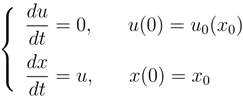
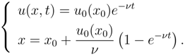
The most simple example is represented by the Burgers equation:

u_t + uu_x = 0,   u(x, 0) = u₀(x)

(13)

which, using the characteristics method, can be rewritten as

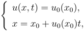
and admits the general solution:

(14)

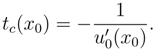
in which, u is a function of (x, t) through the parameter x₀. The invertibility between x₀ and x in (14)₂ is lost at the time

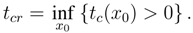
The critical time is the smallest positive value of t_c(x₀):

If instead of (13), we take into account a dissipative production term like

u_t + uu_x = −νu,  u(x, 0) = u₀(x)

with ν = constant > 0, then we have

which admits the solution

and we obtain

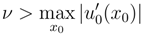
Therefore if

the classical solution exists for all the times: the dissipation dominates with respect to the hyperbolicity. Otherwise, if

the hyperbolicity dominates the dissipation and, in general, we do not have global existence of smooth solution.

Unfortunately, the physical systems are of mixed type, some equations are conservation laws and the others are real balance laws (see (12)), i.e. we are in the case in which

In this case, the coupling condition discovered for the first time by Kawashima and Shizuta (K-condition) [15] such that the dissipation present in the second block has effect also to the first block of equation plays a very important role for global existence of smooth solutions. The condition reads:

In the equilibrium manifold any characteristic eigenvectors r are not in the null space of ∇f , i.e.

(15)

In fact, if the system of balance laws is endowed with a convex entropy law and is dissipative, the K-condition becomes a sufficient condition for the existence of global smooth solutions provided that the initial data are sufficiently smooth. Hanouzet and Natalini [16] in one dimensional space and Yong [17] in the multidimensional space, have proved the following theorem:

Assume that the system is strictly dissipative and the K-condition is satisfied. Then there exists δ > 0, such that, if ∥u(x, 0)∥₂ ≤ δ, there is a unique global smooth solution, which verifies

u ∈ $𝒞$⁰([0, ∞); H²(ℝ) ∩ $𝒞$¹ ([0, ∞); H¹(ℝ)) .

Moreover Ruggeri and Serre [18], have proved in the one-dimensional space that the constant states are stable:

Under natural hypotheses of strongly convex entropy, strict dissipativeness, genuine coupling and “zero mass” initial for the perturbation of the equilibrium variables, the constant solution stabilizes

∥u(t)∥₂ = O (t₋^1/2) .

Recently, Lou and Ruggeri [19] have observed that the weaker K-condition for which (15) is required only for the right eigenvectors corresponding to genuine non-linear waves is a necessary (but not sufficient) condition for the global existence of smooth solutions.

5. The extended thermodynamics

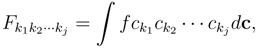
In the kinetic theory the macroscopic thermodynamic quantities are identified as moments of the phase density

(16)

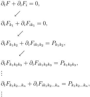
and due to the Boltzmann equation (3), the moments satisfy an infinite hierarchy of balance laws in which the flux in an equation becomes the density in the next one:

By taking into account that P_kk = 0, the first five equations are conservation laws and coincide respectively with the mass, momentum and energy conservation, while the other equations are balance laws.

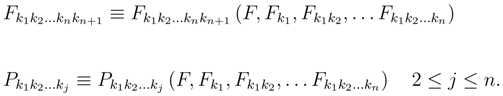
When we cut the hierarchy at the density with tensor of rank n, we have the problem of closure because the last flux end the production terms are not in the list of the densities.

The first idea of modern rational extended thermodynamics (Müller and Ruggeri [20]), was to view the truncated system as a phenomenological system of continuum mechanics and then to consider the new quantities as constitutive functions:

According to the continuum theories, the restrictions on the constitutive equations come only from universal principles, i.e.: entropy principle, objectivity principle and causality and stability (convexity of the entropy).

The restrictions are so strong (in particular the entropy principle) that, at least, for processes not too far from the equilibrium, the system is completely closed and, in the case of 13 moments, the results are in perfect agreement with the kinetic closure procedure proposed by Grad [21].

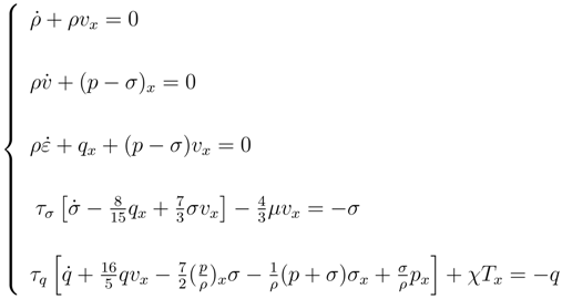
By using usual symbols (the dot indicate the material derivative), the 13-moments Grad system in the one-dimensional are:

We observe that if the relaxation times τ_σ = τ_q = 0 the last two equations reduces to the classical Navier-Stokes and Fourier equations respectively. Therefore from physical point of view the extended thermodynamics (ET) allows to understand that classical constitutive equations are an approximation of balance laws when relaxation times are negligible. This important result infers that the new differential system is hyperbolic instead to be parabolic as in classical theory and this fact eliminates the so-called heat paradox.

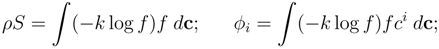
Unfortunately, for rarefied gases we have discovered that in limit situations as high frequencies for sound waves, or special angles for light scattering, or large Mach number in shock waves, the 13–moment theory gives better results with respect to the Fourier-Navier-Stokes one, but its predictions are unsatisfactory when the results coming from the theory are compared to experiments. In such situations we need more moments. In this case it is too difficult to proceed with a pure macroscopic theory (as the

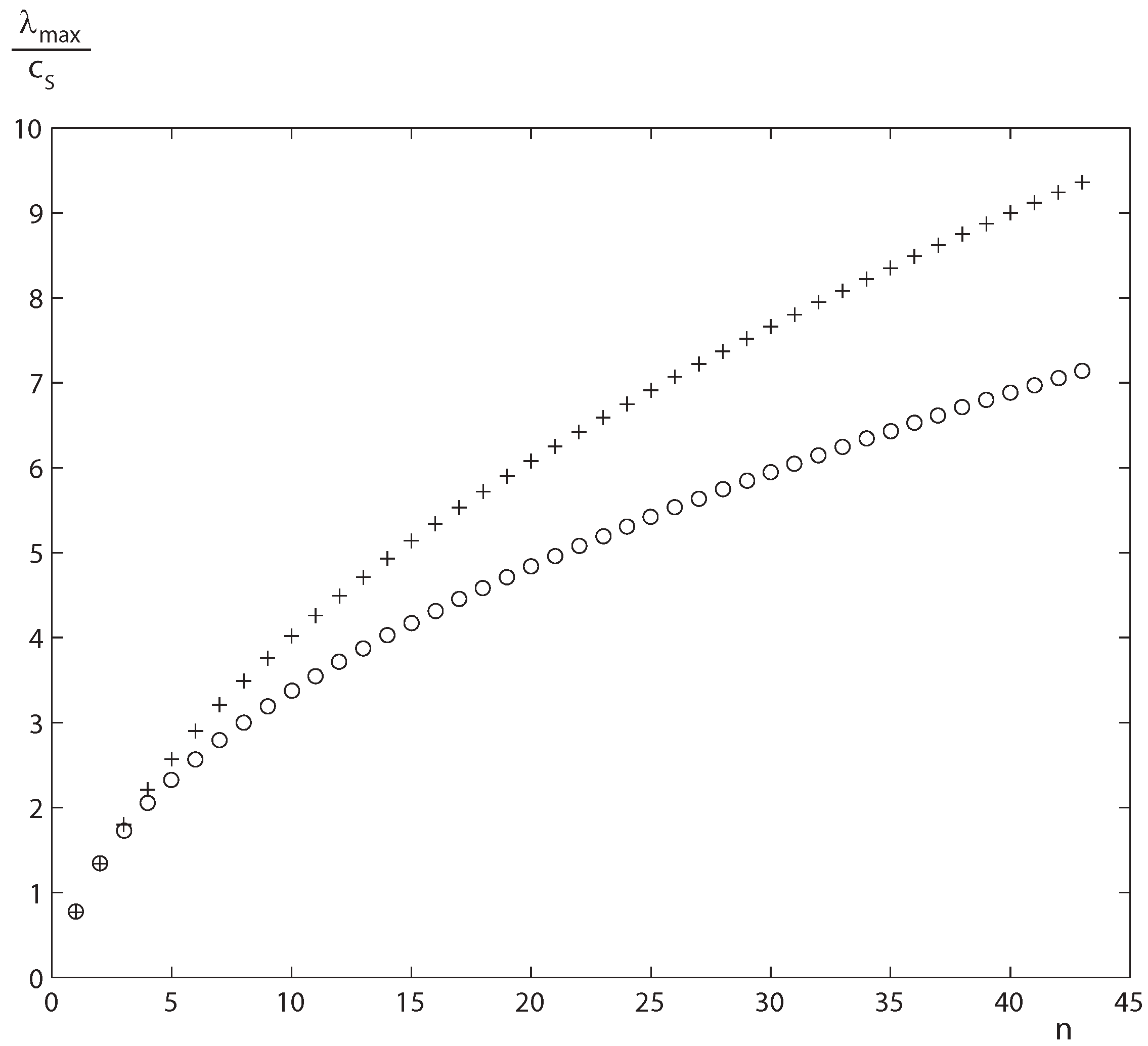
Figure 2. The maximum characteristic velocity as function of index of truncation of moments in sound unity and the lower bound (17).

Figure 2. The maximum characteristic velocity as function of index of truncation of moments in sound unity and the lower bound (17).

13–moments theory) and it is necessary to recall that the F’s are moments of a distribution function f (see (16)). The problem consists int this case to determine a truncated distribution function f_n such that the truncated system of order n satisfy the entropy principle . This closure procedure is possible to prove that is equivalent to the so-called Maximization of entropy method that consist to determine f_n requiring that the entropy density have a maximum under the constraints of fixed values for the moments until tensorial index n. (see for details [22], [20], [23])

Now that we have stated, that for any n we may use the closure of ET, the following question arises: what kind of relation does exist between two closure theories with different index, a theory S_n and a theory S_m with n > m? Boillat and Ruggeri [10] have proved that S_m is a principal subsystem of S_n. In particular, the Euler systems become the equilibrium subsystem of any ET theory.

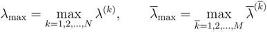
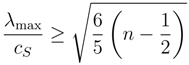
Moreover, according to the subcharacteristic conditions (10) it is possible to deduce a lowest bounding expression for the maximum characteristic velocity in sound velocity unity [22]:

(17)

where λ_maxis the maximum characteristic velocity evaluated at equilibrium and c_S is the sound velocity. Therefore, λ_max becomes unbounded when n tends to ∞ (see Figure 2).

Moreover, it is possible to prove that the K-conditions are satisfied and therefore for small initial data global smooth solutions of ET exist for every time and converge to an equilibrium state [24].

The success of the Extended thermodynamics was verified in several circumstances with a very good agreement with experiments. That are the cases for

• light scattering phenomena and linear sound waves in the high frequencies limit (see [20]),
• the existence of shear stress also in static solutions with radial symmetries [25],
• the hydrodynamical models of semiconductors [26], etc.

6. The mixture theory

A similar mathematical structure of ET is the differential system of a mixture of fluids.

A description of simple homogeneous mixtures in the context of rational thermodynamics relies on the postulate that each constituent obeys the same balance laws as a single fluid. They express the rates of change of mass, momentum and energy with appropriate production terms due to the mutual interaction of constituents:

(18)

with ρ_α denoting the density, v_α the velocity, ε_α the internal energy, t_α = −p_α + σ_α the stress tensor and q_α the heat flux of the α constituent of the mixture.

Due to the conservation of mass, momentum and energy of the whole mixture the production terms must satisfy the following relations:

By a proper choice of field variables the balance laws (18) have to be adjoined to the constitutive equations in order to close the system and make it compatible with the second principle of thermodynamics. Let us give a brief review of the models which could be proposed in the mixture theory.

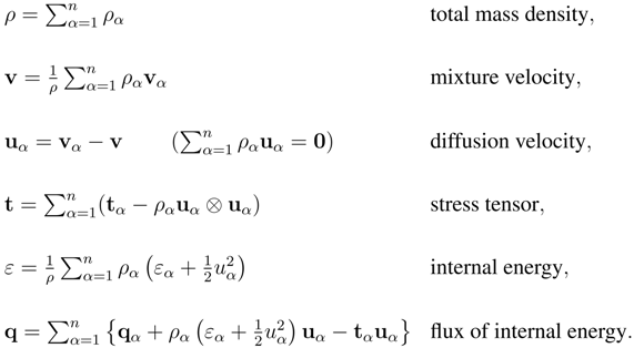
Firstly, from Eq. (18) one may obtain the conservation laws of mass, momentum and energy for the total mixture through the summation of the balance laws and the introduction of following quantities:

In such a way, the conservation laws read:

The system (18) can be rewritten in the equivalent form:

(19)

In this case we have a multi-temperature mixture and the unknown field is

u = (ρ_α, v_α, T_α)^T .

Due to the difficulties to measure the temperature of each component, a common practice among engineers and physicists is to consider only one temperature for the mixture. When we use a single temperature (ST), Eq. (19)₆ disappears and we get a unique global conservation of the total energy in the form (19)₃ (see for example [20]). In this case the unknown field of variables is

u = (ρ_α, v_α, T)^T .

In a recent paper, Ruggeri and Simić [27] discussed the mathematical difference between the ST and the multi temperature (MT) models when the fluid components are Eulerian gases (q_α = 0, σ_α = 0). They proved that the differential system of the ST model is a principal sub-system of the MT model and for large time, MT solutions converge to ST ones. Moreover in the ST case the K-condition and the weak K-condition are both violated and this means that no global smooth solutions can exist for all time. Instead, in the MT case it is easy to verify that K-condition is satisfied for all the eigenvalues. The previous theorems allow to deduce that if the initial data are smooth enough, there exist global smooth solutions at every time and the solutions converge to an equilibrium state. This means that the MT case is a more appropriate model than the ST one.

A noticeable consequence of the previous theorems are that when the temperatures of constituents are different at the initial time they tend for large t to a common equilibrium temperature. In the case of multi-temperatures, we quote recent studies by Ruggeri and coworkers which define a natural average temperature [28], [29] and verify how it is possible to determine the different temperatures when the relaxation times are negligible [30], [29].

7. Conclusions

The entropy principle plays an important role for selecting the physical constitutive equations, to restore the uniqueness for weak solutions, to identify symmetries and nesting structure, to establish the well-posedness of the Cauchy problem and to construct rational models of non-equilibrium thermodynamics.