Shades between Black and Green Investment: Balance or Imbalance?

Abstract

This paper analyses the links established between environmental indices and the oil price adopting a double perspective, long-term and short-term relationships. For that purpose, we employ the Bounds Test and bivariate conditional heteroscedasticity models. In the long run, the pattern of behaviour of environmental indices clearly differed from that of the oil prices, and it was not possible to identify cointegrating vectors. In the short-term, it was possible to conclude that, in contemporaneous terms, the variables studied tended to follow similar paths. When the lag of the oil price variable was considered, the impacts produced on the stock market sectors were partially of a negative nature, which allows us to suppose that this variable plays the role of a risk factor for environmental investment.

1. Introduction

For a long time, business management models adopted the financial perspective. Over the past few decades, however, management models have changed, to accommodate the different stakeholder objectives. Milton Friedman’s proposal that a company’s sole mission is to maximize shareholder value has been questioned by several studies [1,2].

The combined effect of the financial crisis, the diffusion of information about the consequences of global warming, concerns about water scarcity, issues related to human rights and poverty, scandals in governance, environmental disasters, among other aspects, have helped to change the way stakeholders value the integration and management of issues related to sustainability, with investment tending to generate added value in the long run.

Nowadays, an increasing number of organizations consider social and environmental factors when defining their strategy. According to Porter and Kramer [3], when organizations do not consider the different perspectives of stakeholders, there are negative consequences for business competitiveness, in the medium and long terms. In turn, financial markets have progressively incorporated new investment alternatives, in line with this new management model.

There is growing evidence that investors are willing to incorporate these issues into their investment decisions [4]. This implies that investors seek to maximize the financial return on their investments, without forgetting the sustainability of society [5,6]. This awareness of the importance of sustainability-related issues may have been the origin of the creation of sustainable stock market indices, which increasingly attract the attention of investors [7,8,9].

So-called socially responsible investment (SRI), also known as ethical investment or sustainable investment [10], is currently of great relevance. As pointed out by the United Nations [11], in order to achieve the global sustainability goals for the year 2030, the role of investors in financial markets is fundamental, because their resources can help to change the world.

Meanwhile, sustainable investment is a broad concept that covers other more specific types of investment such as the so-called impact investment, that combines financial objectives with social ones (labour and human rights, among others). Nevertheless, we have to highlight so-called green investment, which considers environmental objectives (environmental policies, external/internal management systems, climate change indicators, emissions, solid waste, water, among others) in addition to financial ones [12]. This type of investment has attracted the attention not only of investors but also of all stock market participants. As a result, many financial products associated with green investment have emerged, such as environmental indices [13].

However, despite the great interest in the green investment sector, few scientific studies analyse the behavioural mechanisms of this type of investment, to understand whether its behaviour is guided by its own rules or if, on the contrary, it is influenced by other sectors.

Meanwhile, despite all efforts to minimise the economic dependence on oil, through a strong commitment to renewable energy, it remains dominant and corresponds to practically one third of global energy needs [14,15], so changes in the prices of this raw material produce strong economic and environmental impacts. Several scientific studies confirm the impacts of changes in oil prices, both in macroeconomic terms [16,17], and in equity investment [18,19,20,21,22].

By analysing previous empirical evidence, it is possible to conclude that although several studies have been carried out on the links between oil prices and international stock markets, they have tended to favour, above all, traditional capitalizations, based on a purely financial logic, creating a research gap. This gap results from the fact that, firstly, environmental indices were ignored, and secondly, the two-time horizons, short-term and long-term, were not considered.

We believe this study will help to deepen scientific knowledge about the behaviour of green investment in comparison to black investment. More precisely, the aim of this study is to analyse the impact of oil price changes on environmental indices returns (alternative energy, clean technology, green building, sustainable water and pollution prevention); but also studying the nature and magnitude of the response capacity of the environmental indices to changes in oil prices, seeking to capture the momentum effect; understanding whether the connection between oil prices and environmental assets is homogeneous or whether, on the contrary, it is influenced by the sector effect; and understanding whether the relationship established between the two types of asset depends on the time factor.

In order to achieve the research objectives, in methodological terms, we resort to the proposal of Pesaran et al. [23] and estimate multivariate models of conditional heteroscedasticity, which help to analyse these relationships, both in the long term and the short term.

In terms of structure, the paper continues in Section 2 with the literature review, in Section 3 with the methodology, in Section 4 with the description of the data and the presentation of empirical results and in Section 5 with a synthesis of the main conclusions.

2. Materials and Methods

2.1. Literature Review

The pioneering work of Hamilton [24] is a reference in analysing the relationship between oil prices and macroeconomic indicators. Based on this work, some other studies were developed, with most of them concluding that oil prices impact on macroeconomic variables [17,25,26,27,28,29,30,31].

In the past two decades, the relationship between oil prices and stock markets has given rise to several academic studies, to analyze interdependencies and equilibrium relationships between the two investment sectors in the short run and in the long run. In the finance literature, the terms balance or equilibrium have been used to express the existence of a close relationship between variables or to identify the verification of similar behavior patterns among them in the short run and in the long run [31,32]. The analysis of short-term relationships has been used to study contemporaneous and lagged interdependencies between variables, using for that purpose a diversified methodology, namely multivariate models and the concept of causality [32,33,34]. Regarding the analysis of long-term relationships, several scientific works have tried to identify the existence of long-term equilibria, translated into the verification of common stochastic trends between variables, considering a wider set of observations of the sample studied, in many cases involving time lapses of several years [13,31,35].

In general, the studies about short-run relationships have concluded on a negative relationship between oil prices and stock market returns [20,21,22,36,37,38,39,40,41,42,43,44,45,46].

Despite the attempt to examine the connections between oil prices and stock market indices, the overwhelming majority of studies have not sought to develop the approach in a time-varying environment. Only a few recent works have adopted this type of analysis, using multivariate dynamic conditional correlation models. Additionally, the main academic studies on this issue [18,19,47,48,49,50] concluded that correlation levels between oil prices and equity markets are highly variable over time.

Long-term relationships between stock markets and oil prices have also received attention from the academic community. The general conclusions are somewhat homogeneous, with the two types of asset following the same path [34,51,52]. However, in any case, the main traditional stock indices were selected, to the detriment of environmental indices.

There is ample evidence that sustainability has stopped being marginal in the investment world, to become a central element. Evidence of this change is reflected in the United Nations initiative, called the Principles for Responsible Investment (UNPRI). This initiative seeks to integrate the theme of sustainability, including environmental responsibility, in the financial sphere, requiring investors to adopt a set of guiding principles. In 2016, UNPRI reported more than 1700 signatories, including almost 1200 investment managers and investors, representing more than 59 trillion dollars in assets under management, which compares to 4 trillion dollars in 2006 [53]. Another indicator of this trend is provided by the Global Sustainable Investment Alliance (GSIA), which highlights the fact that the value of global sustainable assets has increased significantly over recent years, from a total of 13.3 trillion dollars in 2012 to 30.7 trillion dollars in 2018 [54,55].

Academics and investors’ interest in the topic of socially responsible investment will have helped to create several stock indices related to sustainability criteria. The first sustainable index was the Domini 400 Social Index (DSI) which was created in 1990. More recently, in the last decade and a half, several other sustainable indices have emerged, such as the Dow Jones Sustainability Index (DJSI), FTSE4Good Index and Morgan Stanley Capital International (MSCI) indices.

Many scientific studies on sustainable investment have focused on financial performance differences between conventional and sustainable investment. Until now, few scientific studies have investigated the behaviour of socially responsible indices [56,57]. The former analysed the short-term dynamics between socially responsible indices, concluding that these dynamics have increased over time. The latter analysed the dynamics generated between environmental indices, both in the short-term and the long-term, concluding that, in the short-term, indices interact very closely, which does not allow differentiating their behaviour from conventional indices. In the long-term, no equilibrium relationships were found between the stock indices.

In the following sections, we address the research gap identified in the previous section, differentiating our work from other studies, considering both two-time horizons and several environmental indices.

Based on the literature analysed, two research hypotheses have been formulated:

Hypothesis 1.

Environmental indices maintain long-run balance relationships with oil prices.

Hypothesis 2.

Environmental indices maintain short-run balance relationships with oil prices.

2.2. Cointegration Test

Pesaran et al. [23] proposed the ARDL test, also called the Bounds Test. The main advantages of this test are in the way it deals with endogeneity issues and the order of integration of the variables. In the first case, the test makes it possible to avoid the problem of endogeneity, since all variables are assumed to be endogenous. In the second case, it allows accommodating variables of the orders one and zero, bypassing the structural limitations of other approaches, namely that of Johansen [58]. On the other hand, the main limitation of the Bounds Test is the fact that it cannot accommodate variables of an order greater than one.

For the bivariate case, the ARDL model with error correction mechanism (ECM) can assume the following generalization:

$$\Delta \ln {\mathrm{Y}}_{\mathrm{t}}={\mathsf{\alpha }}_0+{\displaystyle \sum _{\mathrm{i}=1}^{\mathrm{p}}{\mathsf{\delta }}_1}\Delta {\mathrm{X}}_{\mathrm{t}-\mathrm{i}}+{\displaystyle \sum _{\mathrm{i}=1}^{\mathrm{q}}{\mathsf{\delta }}_2}\Delta {\mathrm{Y}}_{\mathrm{t}-\mathrm{i}}+{\mathsf{\alpha }}_1\ln {\mathrm{Y}}_{\mathrm{t}-1}+{\mathsf{\alpha }}_2\ln {\mathrm{X}}_{\mathrm{t}-1}+{\mathsf{\epsilon }}_{\mathrm{t}}$$

(1)

where $\Delta$ is the operator of the first difference, ${\mathrm{Y}}_{\mathrm{t}}$ is the dependent variable, ${\mathrm{X}}_{\mathrm{t}}$ is the independent variable, ${\mathsf{\alpha }}_0$ is the model constant, ${\mathsf{\delta }}_1$ and ${\mathsf{\delta }}_2$ are the short-term dynamic coefficients, ${\mathsf{\alpha }}_1$ and ${\mathsf{\alpha }}_2$ are the long-term multipliers and $\mathsf{\epsilon }$ is the random disturbance.

The null hypothesis of non-cointegration between the variables studied is given by ${\mathrm{H}}_0:{\mathsf{\alpha }}_1={\mathsf{\alpha }}_2=0$, against the alternative hypothesis, ${\mathrm{H}}_a:{\mathsf{\alpha }}_1\ne {\mathsf{\alpha }}_2\ne 0$, that the variables are not cointegrated.

2.3. Multivariate Models of Dynamic Conditional Correlation

In order to analyse the contemporary and lagged dynamic relationships established between the two variables studied, we estimate two multivariate models of conditional heteroscedasticity, namely the GARCH-BEKK and GARCH-DCC-DECO variants, seeking to ensure parsimony in the estimates produced while meeting the usual Akaike and Schwarz information criteria. In this research work, we have selected the multivariate models of conditional heteroscedasticity, which allow us to adequately accommodate the issue of time-varying volatility, usually present in financial series, as well as to analyze the variable nature of the correlations established between the variables studied [13,33,47,48,49,50].

The GARCH-BEKK model, proposed by Engle and Kroner [59], overcomes the limitations associated with some multivariate models, in terms of complexity, difficulty of estimation, and redundancy of parameters. This model is an evolution of the GARCH-Vech model and is a more parsimonious alternative to multivariate inference.

The GARCH-BEKK representation can be written as follows:

$${\mathrm{H}}_{\mathrm{t}}={\mathrm{C}}^{\prime }\mathrm{C}+{\mathrm{A}}^{\prime }{\mathsf{\epsilon }}_{\mathrm{t}-1}{{\mathsf{\epsilon }}^{\prime }}_{\mathrm{t}-1}\mathrm{A}+{\mathrm{B}}^{\prime }{\mathrm{H}}_{\mathrm{t}-1}\mathrm{B}$$

(2)

where C is an 2 × 2 upper triangular matrix with three parameters and A and B are squared matrices of parameters. ${\mathrm{H}}_{\mathrm{t}}$ is the time varying covariance matrix and is defined as positive by construction, because C is defined positive and the remaining terms are expressed as positive defined quadratic forms. Therefore, we consider the following model:

$${\mathrm{H}}_{\mathrm{t}}={\mathrm{C}}^{\prime }\mathrm{C}+[\begin{array}{l}{\mathrm{A}}_{11}\\ {\mathrm{A}}_{21}\end{array}{\begin{array}{l}{\mathrm{A}}_{12}\\ {\mathrm{A}}_{22}\end{array}]}^{\prime }\left[\begin{array}{cc}{\mathsf{\epsilon }}_{1,\mathrm{t}-1}^2& {\mathsf{\epsilon }}_{1,\mathrm{t}-1}{\mathsf{\epsilon }}_{2,\mathrm{t}-1}\\ {\mathsf{\epsilon }}_{2,\mathrm{t}-1}{\mathsf{\epsilon }}_{1,\mathrm{t}-1}& {\mathsf{\epsilon }}_{2,\mathrm{t}-1}^2\end{array}\right][\begin{array}{l}{\mathrm{A}}_{11}\\ {\mathrm{A}}_{21}\end{array}\begin{array}{l}{\mathrm{A}}_{12}\\ {\mathrm{A}}_{22}\end{array}]+[\begin{array}{l}{\mathrm{B}}_{11}\\ {\mathrm{B}}_{21}\end{array}{\begin{array}{l}{\mathrm{B}}_{12}\\ {\mathrm{B}}_{22}\end{array}]}^{\prime }{\mathrm{H}}_{\mathrm{t}-1}[\begin{array}{l}{\mathrm{B}}_{11}\\ {\mathrm{B}}_{21}\end{array}\begin{array}{l}{\mathrm{B}}_{12}\\ {\mathrm{B}}_{22}\end{array}]$$

(3)

The MGARCH-DECO model was introduced by Engle and Kelly [60], to describe the dynamic equicorrelations established between several international stock markets. The MGARCH-DECO model can be specified as:

$${\mathrm{R}}_{\mathrm{t}}=\left(1-{\overline{\mathsf{\rho }}}_{\mathrm{t}}\right){\mathrm{I}}_{\mathrm{n}}+{\overline{\mathsf{\rho }}}_{\mathrm{t}}{\mathrm{J}}_{\mathrm{n}\mathrm{x}\mathrm{n}}$$

(4)

$${\overline{\mathsf{\rho }}}_{\mathrm{t}}=\frac{2}{\mathrm{n}\left(\mathrm{n}-1\right)}{\displaystyle \sum _{\mathrm{i}\ne \mathrm{j}}\frac{{\mathrm{q}}_{\mathrm{i}\mathrm{j},\mathrm{t}}}{\sqrt{{\mathrm{q}}_{\mathrm{i}\mathrm{j},\mathrm{t}}{\mathrm{q}}_{\mathrm{i}\mathrm{j},\mathrm{t}}}}},\mathrm{i},\mathrm{j}$$

(5)

$${\mathrm{Q}}_{\mathrm{t}}=\left(\overline{\mathrm{Q}}-{\mathrm{a}}_2\overline{\mathrm{Q}}-{\mathrm{b}}_2\overline{\mathrm{Q}}\right)+{\mathrm{a}}_2{\mathrm{z}}_{\mathrm{t}-1}{{\mathrm{z}}^{\prime }}_{\mathrm{t}-1}+{\mathrm{b}}_2{\mathrm{Q}}_{\mathrm{t}-1}$$

(6)

where ${\mathrm{I}}_{\mathrm{n}}$ is the n-dimensional identity matrix and ${\mathrm{J}}_{\mathrm{n}\mathrm{x}\mathrm{n}}$ is the matrix of ones, ${\overline{\mathsf{\rho }}}_{\mathrm{t}}$ is the equicorrelation, which can be calculated as the average of the $\frac{2}{\mathrm{n}\left(\mathrm{n}-1\right)}$ dynamic correlations at moment t, implying that the equicorrelation represents the mean of conditional correlations.

Estimation of the parameters of the MGARCH-DECO model uses the quasi-maximum likelihood estimation. The maximization function is:

$$\mathsf{\tau }\left(\mathsf{\theta }\right)=\frac{1}{\mathrm{T}}{\displaystyle \sum _{\mathrm{t}=1}^{\mathrm{T}}\left(\log \left[{\mathrm{R}}_{\mathrm{t}}\right]+{{\mathsf{\epsilon }}^{\prime }}_{\mathrm{t}}{\mathrm{R}}_{\mathrm{t}}^{-1}{\mathsf{\epsilon }}_{\mathrm{t}}\right)}$$

(7)

2.4. Data

In order to satisfy the research objectives, daily data are used, covering a period of approximately 11 years, considering Brent prices and five environmental indices, namely:

−

Alternative energy (EA)—composed of small, medium and large companies in emerging and developed markets, for which at least 50% of their revenue comes from the sale of products and services that contribute to generating capacity, based on renewable and clean resources;

−

Clean technology (TL)—composed of small, medium and large companies in emerging and developed markets, for which at least 50% of their revenue comes from the sale of products and services related to clean technologies;

−

Green construction (CV)—composed of small, medium and large companies in emerging and developed markets, for which at least 50% of their revenue comes from the sale of products and services that respect green construction standards;

−

Pollution prevention (PP)—composed of small, medium and large companies in emerging and developed markets, for which at least 50% of their revenue comes from the sale of products and services related to pollution prevention, waste minimization, recycling and treatment systems;

−

Sustainable water (AS)—composed of small, medium and large companies in emerging and developed markets, for which at least 50% of their revenue comes from the sale of products and services related to water treatment and the minimization of its waste, water infrastructures, water resource management and efficiency systems.

The data related to the environmental indices were collected from Morgan Stanley Capital International, covering the period from January 2009 to November 2020 and corresponding to 3003 daily observations.

To develop our analysis, for all variables, we consider levels and returns series. We calculate the daily returns for each variable, ${\mathrm{r}}_{\mathrm{t}}$, using the following formula: $\ln \left({\mathrm{P}}_{\mathrm{t}}/{\mathrm{P}}_{\mathrm{t}-1}\right)$, where ${\mathrm{P}}_{\mathrm{t}}$ and ${\mathrm{P}}_{\mathrm{t}-1}$ are the series of closing prices on days $\mathrm{t}$ and t − 1, respectively.

2.5. Descriptive Analysis and Stationarity

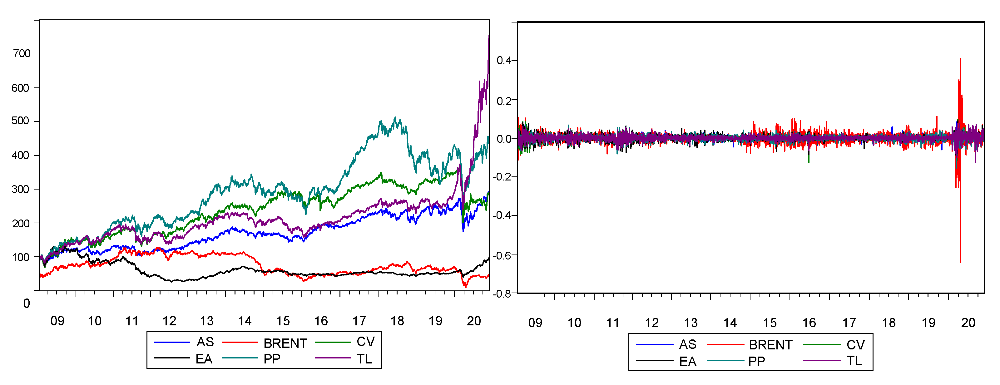
Figure 1 shows the evolution of the series formed by oil prices and the indices in levels (on the left), as well as the respective logarithmic return series (on the right), in the period from October 2009 to November 2020.

The graphical analysis of the series in levels suggested that throughout the sample period of approximately 11 years some environmental indices have shown identical patterns, especially those related to clean technology (TL), green building (CV), pollution prevention (PP) and sustainable water (AS). Alternative energy (EA) and Brent price series follow each other closely.

The analysis of the return series suggests a first indication that all the series may be stationary. In any case, in no case does the graphical analysis infer the relationships established between the variables. Therefore, in the next section, the comovements between the series will be analysed, based on the conditional correlations generated from the multivariate conditional heteroscedasticity models.

The main descriptive statistics of the series are contained in

Table 1. Descriptive statistics.

	AS	BRENT	CV	EA	PP	TL
Mean	0.00037	0.00004	0.00037	0.00001	0.00052	0.00069
Median	0.00073	0.00035	0.00067	0.00029	0.00105	0.00075
Maximum	0.08402	0.41202	0.09553	0.08875	0.06981	0.07631
Minimum	−0.12513	−0.64370	−0.12463	−0.11400	−0.15520	−0.12648
Standard deviation	0.01301	0.02854	0.01331	0.01527	0.01415	0.01374
Asymmetry	−0.51940	−2.95999	−0.82080	−0.45699	−0.65955	−0.40431
Kurtosis	11.97665	116.03321	15.98329	7.96437	10.10714	10.85707
JB (Prob.)	(0.00000)	(0.00000)	(0.00000)	(0.00000)	(0.00000)	(0.00000)
ADF (Levels)	(0.84702)	(0.51967)	(0.28522)	(0.62855)	(0.60050)	(1.00000)
ADF (Prof.)	(0.00000)	(0.00000)	(0.00010)	(0.00010)	(0.00010)	(0.00010)

Note: Values in parentheses indicate the p-value.

. Analysis of these statistics allows a first conclusion that all series have positive average returns.

All the series analysed showed signs of deviation from the normality hypothesis, when comparing the asymmetry and kurtosis coefficients with the reference values (zero and three, respectively). The previous indication was confirmed, more robustly, by applying the Jarque-Bera test. Table 1 presents the statistical probabilities. In any case, considering the results, it is possible to conclude that all the series considered are statistically significant at 1%, clearly rejecting the normality assumption.

Tests for stationarity were performed on each variable using the augmented Dickey-fuller (ADF) tests. The null hypothesis (H₀) is that the variables are non-stationary or they have a unit root I(1). The alternative hypothesis (H_a) is that the variables are stationary or they do not have a unit root I(0). The results of these stationarity tests are shown in

Table 2. Summary of the bounds test results.

Variables	ARDL Model	F-Statistic
EA/Brent	(1;1)	1.503613
TL/Brent	(1;1)	2.636126
CV/Brent	(1;2)	2.789922
PP/Brent	(1;2)	1.288165
AS/Brent	(4;4)	1.385121

Notes: In the study of bivariate relations, the critical values of the Bounds Test of 6.84 and 7.84 were taken into account for the lower limit I(0) and the upper limit I(1), respectively, according to Pesaran et al. [21].

. The lag length was determined by the Bayesian criterion. For both environmental stocks and oil prices, considering the series of returns, the ADF test supports stationarity at a 1% level of significance, contrary to what was found for the series in levels, which proved to be integrated and therefore not stationary.

3. Results

In order to identify the possible occurrence of long-term equilibrium relationships between the environmental indices and the Brent price, we applied the approach of Pesaran et al. [23], for each bivariate case.

The application of the Bounds Test implies that the series studied do not have an integration order greater than 1, although they may have a different integration order. Taking into account the results of the ADF unit root tests, reported in Table 1, in all cases the series in levels are I(1), which guarantees fulfilment of the assumptions required by the test.

Regarding application of the Pesaran et al. [23] approach, we started by testing different formulations for different lags. The quality of each formulation was evaluated, taking into account the Akaike and Schwarz information criteria. At the same time, the F statistic, presented in Table 2, was calculated in order to test whether the joint significance of the coefficients of the lagged variables is significantly different from zero, that is, whether the ECM is significant and, consequently, admitting the presence of cointegration. The value of the F statistic was compared with the limits of the critical values, provided by Pesaran et al. [23]. These critical values are defined for several different cases, which result from the inclusion of constant and/or trend, as well the level of significance selected, implying consideration of lower and upper limits. For the purpose of analysis, the 1% confidence level was selected. According to Pesaran et al. [23], when the value of the F statistic is less than the lower limit, we may conclude that there is no cointegration. When the value of the F statistic is greater than the upper limit, we may conclude that cointegration exists. Finally, when the value of the F statistic is between the lower and upper limits, there is an inconclusive test.

Table 2 reports the optimal lag structure, for the different models estimated, taking into account the Akaike and Schwarz information criteria, as well as the values of the F statistic, which reflects the joint significance of the coefficients of the lagged variables at levels. All the statistics associated with the bivariate cases were below the lower limit, at 1% significance, whereby the hypothesis of cointegration between the pairs of variables studied is rejected for all equations. Therefore, these results are not in line with those obtained for conventional indices in earlier research [38,51,52].

In order to check the robustness of the results obtained, the Johansen proposal was considered [58], which is translated in the tests of cointegration (tests of the trace and maximum Eigen value). In either case, the bivariate relationships did not identify cointegrating vectors, in consistency with the results generated through the Bounds Test.

From a theoretical and practical point of view, we believe our results have several relevant implications.

Firstly, from a theoretical point of view, the absence of long-term equilibrium relationships between the variables studied confirms the assumptions of the market efficiency hypothesis [61]. Therefore, for the long term, it was not expected that Brent prices would help to predict the behaviour of environmental segments.

Secondly, from a practical perspective, the results allow rejection of hypothesis 1, as no long-term equilibrium relationships were found, which leads us to believe that the environmental segments and the Brent price are not guided by the same behavioural mechanisms, which would restrict the independence of movements and give rise to partially predictable behaviour. As a common long-term stochastic trend between “green investment” and “black investment” has not been identified, the consideration of environmental segments for an international investment strategy appears to be an interesting possibility, insofar as it allows expansion of diversification alternatives.

In order to analyse the short-term equilibrium relationships between environmental indices and the Brent price, several bivariate conditional heteroscedasticity models were estimated based on the return series, after checking the stationarity of the series by applying the ADF tests (Table 1).

The analysis of bivariate relationships involved the estimation of two models (GARCH-DCC-DECO and GARCH-BEKK), seeking to respect their respective specific assumptions, taking into account several specifications, namely the asymmetric effect, the size of the lag in the volatility equation, and the distribution of errors. As none of these specifications showed the ability to improve the models’ performance, we opted for its simpler versions.

Considering the results of the Schwarz and Akaike information criteria, the GARCH-DCC-DECO model was the one that, in general, best fitted the data. However, it was not always possible to comply with the specific assumptions of this model, especially with regard to guaranteeing the validity of the conditional correlation matrix, which led to selecting the GARCH-BEKK model.

For the sake of checking the robustness of the results obtained, two different procedures were considered.

Firstly, the multivariate models were estimated considering weekly data. The results obtained from these data proved to be consistent with those obtained for daily data, with no change in the dynamics generated between the variables studied.

Secondly, several specifications of the multivariate models were considered, with the varying correlations generated for these specifications proved to be intensely correlated with those obtained through the models presented in

Table 3. Summary of the GARCH models.

	Contemporary Analysis	Lagged Analysis
EA/Brent	GARCH-DCC-DECO	GARCH-BEKK (Scalar)
TL/Brent	GARCH-DCC-DECO	GARCH-BEKK (Scalar)
CV/Brent	GARCH-DCC-DECO	GARCH-BEKK (Scalar)
PP/Brent	GARCH-DCC-DECO	GARCH-BEKK (Scalar)
AS/Brent	GARCH-DCC-DECO	GARCH-BEKK (Scalar)

Notes: This table presents the summary of the models selected for each bivariate situation, taking into account the fulfillment of the specific assumptions of the models, as well as the results of the Akaike and Schwarz information criteria. Considering the multiplicity of estimates produced, the authors choose not to include them fully in the present work, showing only the dynamic conditional correlations generated from the estimates produced by the models in question. If the reader is interested in accessing these estimates, they are available from the authors upon request.

.

Table 3 presents a summary of the selected bivariate models resulting from the interaction between environmental indices and Brent prices, for the contemporary and lag scenarios.

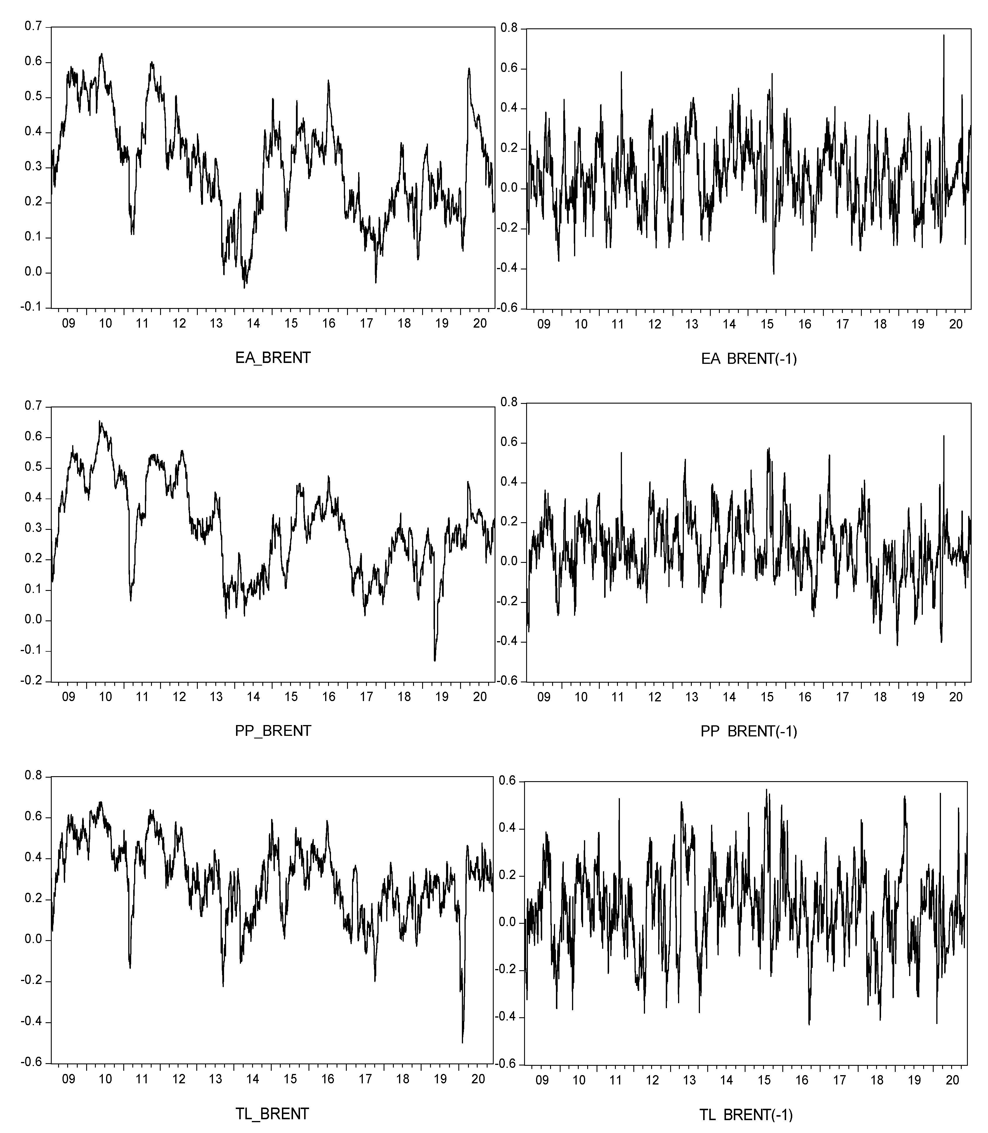
Based on the estimates of the bivariate models, Figure 2 presents the varying correlations between environmental indices and Brent price over time.

For investors and market players, it will be of interest to explore the ability of the Brent price to provide information about the future behaviour of environmental indices. To meet this objective, Figure 2 was created, presenting two different scenarios for each stock market index. On the left, contemporary dynamic correlations between the variables studied are presented; on the right, the lagged dynamic correlations are shown, with the incorporation of the one-day lag in the Brent variable, in order to examine the impact on the environmental segments caused by previous changes in the oil sector.

In both scenarios, the correlations showed marked oscillations throughout the period, which is similar to the conclusions of previous research involving conventional indices, namely those already mentioned in the previous sections [18,19,47,48,49].

4. Discussion

In general, the contemporaneous conditional correlations between environmental indices and the Brent price were positive. The most intense correlations were recorded in 2010, perhaps as a result of the global financial crisis, which emerged in the American subprime sector in 2008 and subsequently spread worldwide as a great recession. This crisis had several consequences, particularly in the financial sector, which was heavily affected, and the Euro sovereign debt crisis, which implied a struggle for Eurozone countries to pay off debts accumulated over decades. There were also severe consequences for European economies, with GDP falling sharply. Certainly, the strongest correlation during the crisis period, between environmental indices and the Brent price, can be explained by the fact that the crisis produced consequences both for stock markets and Brent price sectors, causing a fall in all asset prices. If, on the one hand, the crisis period showed the highest conditional correlations, on the other hand, it reported several days of simultaneous extreme correlations. Taking into account the proposal of Singh et al. [62], Tippett et al. [63], Li et al. [64] and Taszarek et al. [65], according to which the extreme values are provided by the 99th percentile, it is possible to conclude that the month of May 2010 reported a sequence of several days with simultaneous extreme correlations, allowing the idea of transversal linkages between the oil sector and environmental segments, especially during very turbulent periods.

Based on the results obtained, we believe that hypothesis 2 is partially confirmed. In certain periods, especially those of high turbulence, environmental segments and the oil sector follow relatively close pathways, implying a relationship based on a certain balance in the short-term. The results obtained, however, did not allow us to confirm the general conclusions of other research, namely Bein and Aga [20], Ciner [46], Filis and Chatziantoniou [21], and Kurshid and Uludag [22], among others, that there is a negative relationship between the changes in oil prices and the returns of stock market indices. The situations identified in the present study are merely episodic and not open to generalization. On the other hand, the results revealed certain homogeneity in the dynamics between the variables studied. Even the segment related to alternative energy companies, which could be more sensitive to changes in Brent prices, reported a similar bivariate relationship.

Having analysed the hypothesis of changes in environmental segments, caused by impacts from the Brent variable, with a one-day lag, it was possible to conclude that, like contemporary relationships, the correlations showed high variability over time, describing a highly dynamic path, which included positive and negative values. In most of the segments studied, the higher positive correlations occurred in the period corresponding to the pandemic, especially in the first half of March 2020.

Comparing the assumptions of contemporaneity and lead-lag relationship, it is important to highlight three main aspects. The first aspect concerns the decrease of correlation intensity in the second assumption. The second aspect concerns the significant increase in the number of sessions that registered negative correlations. In this regard, the results of this study are partially consistent with those of Filis et al. [48], to the extent that the lagged Brent prices constitute a kind of risk factor for stock markets. The third aspect results from the fact that the number of sessions with extreme simultaneous conditional correlations decreased significantly compared to the assumption of contemporaneity, registering only three sessions in this condition, one of them associated with the beginning of the pandemic crisis.

5. Conclusions

Connections between the oil price and stock markets have motivated several studies. However, the vast majority of these studies have focused on traditional indices, based on a purely financial logic, to the detriment of environmental indices.

This research develops a first comprehensive analysis of the links between environmental equities and the oil sector, representing the “green” and “black” sectors, respectively, in order to analyse the dynamics between them, in the long-term and short-term.

In order to analyse the long-term dynamics, the Pesaran et al. [21,23] approach was applied to each of the five bivariate cases. In no case was it possible to identify long-term equilibrium relationships between the variables studied, which allows us to conclude that the Brent price and environmental stock markets do not show the same pattern of behaviour. The mechanisms generating the behaviour observed seem to be explained by specific factors and not by common factors, offering investors a chance to diversify their investments, taking into account both types of asset and assuming a long-term investment strategy.

In turn, the analysis of the short-term dynamics between the two investment sectors involved the estimation of bivariate conditional heteroscedasticity models, namely the GARCH-DCC-DECO and GARCH-BEKK specifications, in order to analyze the dynamics established between the variables over time for the contemporary and lagged scenarios. The results obtained reveal that, in turbulent periods, environmental segments and the oil market show similar behaviour patterns, reflecting a relatively balanced relationship between the two types of asset. Independent of market conditions, when considering the one-day lag for the oil price variable, the number of market sessions characterized by negative correlation registered a significant increase, suggesting that “black investment” plays a role of risk factors for “green investment”. In general, considering the lagged scenario, the level of conditional correlations decreased significantly.

Considering the results obtained in this study, it does not seem possible to admit that the relationship between the oil price and environmental investment is guided by a full balance. Instead, if there is a close relationship, it will only happen in episodic situations. If we take duration into account the connection between the two variables is verified only in periods of turbulence and does not establish a long-lasting relationship.

Our findings have important implications for policymakers, portfolio managers and investors. The occurrence of simultaneous extreme correlations reveals the presence of systematic risk, which transversely affects both stock market investment and the energy sector. Therefore, we believe that policymakers should consider how changes in global oil prices could affect the dynamics of the environmental stock market segments. International investors and portfolio managers are interested in understanding how shocks in the oil market influence environmental segments and also want to know if these shocks have a similar impact level in the short and long terms. In addition, investors can manage their investments according to various time horizons, since the contagion effects, from the oil sector to environmental segments, can remain for a certain time, so investors are interested in understanding if the relationship between “black investment” and “green investment” changes for different time horizons and for different market conditions. We believe our empirical results can be considered in the fields of investment strategies and portfolio management, incorporating both “black and green” investment sectors, to develop more accurate predictions to assist investment decision-making, as well as providing some guidance for risk managers in designing hedging strategies.

In future research we intend to deepen study of the relationship between environmental indices and the Brent price, applying the model of structural vector autoregression and the concept of spectral causality, which will provide a greater level of detail about the dynamics generated between the two investment sectors. We will also explore new research questions, to analyse the impact of the pandemic crisis on the relationship between the sectors.