Monotonic Functions Method and Its Application to Staging of Patients with Prostate Cancer According to Pretreatment Data

Abstract

Prostate cancer is the second most frequent malignancy (after lung cancer). Preoperative staging of PCa is the basis for the selection of adequate treatment tactics. In particular, an urgent problem is the classification of indolent and aggressive forms of PCa in patients with the initial stages of the tumor process. To solve this problem, we propose to use a new binary classification machine-learning method. The proposed method of monotonic functions uses a model in which the disease’s form is determined by the severity of the patient’s condition. It is assumed that the patient’s condition is the easier, the less the deviation of the indicators from the normal values inherent in healthy people. This assumption means that the severity (form) of the disease can be represented by monotonic functions from the values of the deviation of the patient’s indicators beyond the normal range. The method is used to solve the problem of classifying patients with indolent and aggressive forms of prostate cancer according to pretreatment data. The learning algorithm is nonparametric. At the same time, it allows an explanation of the classification results in the form of a logical function. To do this, you should indicate to the algorithm either the threshold value of the probability of successful classification of patients with an indolent form of PCa, or the threshold value of the probability of misclassification of patients with an aggressive form of PCa disease. The examples of logical rules given in the article show that they are quite simple and can be easily interpreted in terms of preoperative indicators of the form of the disease.

1. Introduction

Machine-learning methods are widely used in modern medicine. These methods have the potential to be used to extract knowledge from medical data to diagnose a disease, determine the severity of a patient’s condition, choose a treatment method, and predict their condition after treatment [1,2,3,4]. Most machine-learning methods are based on general statistical classification models. However, there are problems of diagnostics and forecasting, the features of which are not taken into account in these models. These include the tasks of medical diagnostics with a monotonous relationship between prognostic and predicted indicators: the stronger the deviation of prognostic indicators from the norm, the more serious the predicted degree of the disease. Therefore, for example, in the works [5,6] to determine the severity of the patient’s condition, a model was proposed in which it was assumed that an increase in the deviation of any of the indicators of the patient’s condition from the norm, all other things being equal, increases or does not change (but does not decrease) the severity of the disease. Taking into account the property of monotonicity inherent in such problems would facilitate their more efficient solution.

To solve diagnostic problems with a monotonic relationship between prognostic and predicted indicators, we have developed a method of monotonic functions. In this paper, we consider the method and its application to select one of two types of surgery for prostate cancer based on preoperative data. Prostate cancer (PCa) is the second most common malignant neoplasm (after lung cancer). Globally in 2018, it amounted to 1,276,106 new cases and caused 358,989 deaths (3.8% of all cancer deaths in men) [7]. The choice of appropriate treatment tactics is based on the results of pretreatment staging of PCa.

Research on the indicators of prostate cancer is developing intensively. Studies aimed at identifying the specific features of PCa have identified the diagnostic potential of separate indicators of the disease. These studies have shown the need for the development of multivariate models for diagnosis and determination of the stage of the disease, as well as for the prognosis and choice of treatment tactics. Research related to the development of the Prostate Health Index (PHI) is a very successful example of aggregating prostate cancer indices [8,9,10]. The cycle of works on the Prostate Cancer Risk Assessment Index (CAPRA) is widely known [11,12,13]. The CAPRA Index was designed to facilitate the classification of disease risk when conducting clinical assessments of the likelihood that a given tumor will recur after treatment, progress, and be life-threatening, according to pretreatment data. One of the urgent problems when choosing the type of surgery is the classification of indolent and aggressive forms of PCa in patients with the initial stages of the tumor process. The problem of the classification of patients with indolent and aggressive forms of PCa before treatment was considered in [14,15,16,17,18,19]. In these works, the logistic regression method was used to solve the problem. Five indicators were used for classification. Based on cross-validation data, the algorithm identifies a group of 55% of patients with aggressive PCa in the absence of patients with indolent PCa status. These forms of the disease are ordered. The aggressive form of the disease refers to a more severe form, which is characterized by the presence of a more common tumor process. To solve this problem, we propose to use a new machine-learning method of binary classification, which we called the method of monotonic functions.

We consider the basics of the method of monotonic functions in Section 2 and Section 3. Section 4 describes the experimental modeling and the result of applying the method to the problem of classifying patients with indolent and aggressive PCa.

2. Monotonic Functions Method

Several disciplines study complex processes, exploring the relationship with their simpler properties. Several disciplines study complex processes, exploring the relationship with their simpler properties. At the first stage, the relationship of the process only with individual indicators is studied. At the second stage, it becomes possible to study the relationship of the process with a set of indicators. To evaluate a connection between the process and a set of indicators, machine-learning methods are used.

The main task of machine-learning is to find a classification rule based on a sample of precedents. Most of the methods use the analytical function of properties (indicators or features) of objects for classification. The type of analytical function is selected based on the mathematical model of the problem being solved, and its parameters are found using the learning algorithm. The linear relationship between indicators and classes of objects is approximated by a weighted algebraic sum of indicators. Non-linear dependence is approximated in a wider class of functions. An example of a non-linear relationship between disease severity and indicators of immunochemical analysis of blood is the Prostate Health Index (PHI) function. Usually, when solving a classification problem, the information about the type of analytical function is absent. Statistical methods are used to estimate it.

The problem of choosing the type of analytical function can be bypassed in nonparametric classification methods. In these methods, it is assumed that for each test object, there is a precedent or several precedents of the same class, the indicators of which are closer to this object than the indicators of one or more precedents of the alternative class. The class membership decision is based on the minimum distance to one or more objects in the training class set. Methods of nonparametric classification, similar to the previous parametric ones, require the introduction of a classification model. This is where the model must determine how the distance is calculated (metric). In most cases, a priori knowledge about the choice of a metric in classification problems is usually absent. From statistical considerations, it is known that in the general case, the most successful is the application of the Mahalanobis metric.

Thus, from the above, it can be seen that both methods of teaching classification, in addition to the training sample, need knowledge about the model of the relationship between the estimated value and the used indicators of objects. Such knowledge is available in those problems of medical classification, in which the class number can be associated with the degree of manifestation of the disease. Long-term studies of medical indicators have revealed for each of them the boundaries of the intervals with values that are typical for healthy people. It can be assumed that the smaller the deviation of the indicator from the norm, the less or equal (but not more) the deviation of the degree of manifestation of the disease from the state of a healthy person. This means that deviations of the process from the norm can be represented by monotonic functions of the values of indicators characterizing the exit of the indicators of the process beyond the range of normal values. This knowledge determines the model underlying the method of monotonic functions.

In this article, the method of monotonic functions is used to the binary classification of patients with indolent and aggressive forms of prostate cancer according to pretreatment data. The method uses two obvious assumptions: (1) the degree of manifestation of the disease is less, the less the deviation of the patient’s indicators from the norm, and (2) patients with an indolent form of prostate cancer have a lower degree of manifestation of the disease than patients with an aggressive form. The model of the method is as follows: (1) a patient whose indices differ from the norm is less than or equal to those of at least one patient from a sample of precedents with an indolent form of prostate cancer, also has an indolent form of prostate cancer; (2) a patient who, in at least one indicator, has a deviation from the norm greater than the deviation from the norm of each patient from a sample of precedents with indolent PCa has an aggressive form of PCa.

Machine-learning methods can extract empirical knowledge from medical data that enable two ways to justify a decision: (1) reasoning by the precedent, which consists of the fact that patients with similar values of indicators have the same diagnoses and severity of the disease and, most likely, will respond in the same way to a certain treatment regimen; (2) reasoning by the decision rule in the language of the subject domain. In the first case, empirically selected knowledge is intuitively understandable, has concrete precedent confirmation, but is not verbalized, and depends on the similarity function that determines the proximity of objects. In the second case, knowledge is verbalized, understandable to specialists in the subject area but does not always have specific precedent confirmation. As you can see, these arguments complement each other. Therefore, when solving classification problems, it is desirable to extract knowledge that can justify the decision using two types of reasoning. The method of monotonic functions finds two solutions from the available data: the rule of nonparametric classification by analogy with the precedent and the rule of logical decision, which is formulated in the language of the subject domain.

3. Algorithm

The method of monotonic functions finds two solutions from the available data: the rule of nonparametric classification by analogy with the precedent and the rule of logical decision, which is formulated in the language of the subject domain. The method uses the following data model. There are two forms of the disease (classes) ${\omega }_1$ and ${\omega }_2$. We know of a limited sample of patients. Patients $q=1,2,\dots ,Q_1$ belong to the class ${\omega }_1$, and patients $\overline{q}=1,2,\dots ,Q_2$ belong to the class ${\omega }_2$. Each patient is described by a set of indicators (a set of features). Patients correspond to points of the I-dimensional feature space ${\mathbf{x}}^{\left(q\right)}=\left\{x_i^{\left(q\right)}\right\}$ and ${\mathbf{x}}^{\left(\overline{q}\right)}=\left\{x_i^{\left(\overline{q}\right)}\right\}$, $i=1,\dots ,I$. Let the severity of the disease in patients of class ${\omega }_1$ be lower than that in patients of class ${\omega }_2$. For each feature, the interval $[a_i,b_i]$ of the indicator norm is known. Patients with indices $\mathbf{x}=\left\{x_i\right\}$ whose deviations from the norm are component-wise less than or equal to deviations from the norm in indices of any point ${\mathbf{x}}^{\left(q\right)}\in {\omega }_1$ have a disease severity no more than in a patient with indicators ${\mathbf{x}}^{\left(q\right)}$ (monotonicity condition).

For simplicity of explanation without loss of generality, we further assume that the monotonicity condition consists of the fact that all points $\mathbf{x}$ of the feature space take values either from the intervals of the norms of the indicators, $x_i\in [a_i,b_i]$ or the larger right boundaries of these intervals, $x_i>b_i$. Then, according to the condition of monotonicity, the patient, to whom the point $\mathbf{x}=\left\{x_i\right\}$, $i=1,2,\dots ,I$ corresponds, has a severity of the disease no higher than the severity of the disease in a patient of class ${\omega }_1$ with indicators ${\mathbf{x}}^{\left(q\right)}=\left\{x_i^{\left(q\right)}\right\}$ if $x_i\le x_i^{\left(q\right)}$ for all $i=1,2,\dots ,I$. If at least one indicator $i=1,2,\dots ,I$ occurs, $x_i>x_i^{\left(q\right)}$, then the severity of the patient’s disease is greater than that of a patient with indicators ${\mathbf{x}}^{\left(q\right)}$. The monotonicity condition corresponds to an ideal situation in which all the indicators of objects necessary for classification are present and the values of indicators are measured accurately. In real situations, due to the incomplete description of the differential properties of objects and the inaccuracy in the measurements of indicators, inequalities $x_i\le x_i^{\left(q\right)}$, $i=1,2,\dots ,I$ are not fulfilled for some pairs of objects. This is one of the reasons for misclassification.

Consider a classification algorithm.

With each point of the training sample ${\mathbf{x}}^{\left(q\right)}\in {\omega }_1$, we connect the area of the feature space

$$W^{\left(q\right)}=\{\mathbf{x}:x_i\le x_i^{\left(q\right)},i=1,2,\dots ,I\}.$$

(1)

We call this set the orthant $W^{\left(q\right)}$ with apex at point ${\mathbf{x}}^{\left(q\right)}$. Since the monotonicity condition is not satisfied for all objects, the orthant with apex at point ${\mathbf{x}}^{\left(q\right)}$ can contain $Q_1^{\left(q\right)}$ points of the class ${\omega }_1$ and $Q_2^{\left(q\right)}$ points of the class ${\omega }_2$. Each orthant $W^{\left(q\right)}$ with vertex ${\mathbf{x}}^{\left(q\right)}$ corresponds to three parameters:

$$P_1^{\left(q\right)}=Q_1^{\left(q\right)}/Q_1,$$

(2)

$$P_2^{\left(q\right)}=Q_2^{\left(q\right)}/Q_2,$$

(3)

$$L^{\left(q\right)}=P_1^{\left(q\right)}/(P_2^{\left(q\right)}+1/Q_1{Q}_2),$$

(4)

where $P_1^{\left(q\right)}$ is the probability that the points of the orthant belong to class ${\omega }_1$, $P_2^{\left(q\right)}$ is the probability that the points of the orthant belong to class ${\omega }_2$ in the orthant, and $L^{\left(q\right)}$ is the likelihood ratio, where the term $1/Q_1{Q}_2$ corrects the value of $L^{\left(q\right)}$ when $P_2^{\left(q\right)}=0$.

The machine-learning algorithm consists of the following steps:

1.

Calculate the likelihood ratio estimates for all orthants of the target class $q=1,2,\dots ,Q_1$ and obtain the training set $\{{\mathbf{x}}^{\left(q\right)},L^{\left(q\right)}\}$.

2.

Renumber the orthants $W^{\left(q\right)}$ in accordance with the decrease in the likelihood ratio estimates $L^{\left(1\right)}\ge L^{\left(2\right)}\ge \cdots \ge L^{\left(Q_1\right)}$.

3.

For points of the set $W^{\left(1\right)}$, determine the values of the functions

$$U{\left(\mathbf{x}\right)}^{\left(1\right)}=P_1^{\left(1\right)}$$

(5)

is the probability of a sample point of class ${\omega }_1$ in the orthant $W^{\left(1\right)}$, and

$$V{\left(\mathbf{x}\right)}^{\left(1\right)}=P_2^{\left(1\right)}$$

(6)

is the probability of a sample point of class ${\omega }_2$ in the orthant $W^{\left(1\right)}$. Determine for points from the set $W^{\left(2\right)}\backslash W^{\left(1\right)}$ the values of the functions $U{\left(\mathbf{x}\right)}^{\left(2\right)}$ and $V{\left(\mathbf{x}\right)}^{\left(2\right)}$, where $U{\left(\mathbf{x}\right)}^{\left(2\right)}$ is the probability, which is defined as the ratio of the number of points of class ${\omega }_1$ from the set $W^{\left(1\right)}\cup W^{\left(2\right)}$ to the number of all points $Q_1$ of the training sample of the class ${\omega }_1$; $V{\left(\mathbf{x}\right)}^{\left(2\right)}$ is the probability equal to the ratio of the number of points of class ${\omega }_2$ from the set $W^{\left(1\right)}\cup W^{\left(2\right)}$ to the number of points $Q_2$ of the class of the training sample ${\omega }_2$. Determine for points from the set $W^{\left(3\right)}\backslash (W^{\left(1\right)}\cup W^{\left(2\right)})$ the values of the probabilities $U{\left(\mathbf{x}\right)}^{\left(3\right)}$ and $V{\left(\mathbf{x}\right)}^{\left(3\right)}$, which are calculated from the set $W^{\left(1\right)}\cup W^{\left(2\right)}\cup W^{\left(3\right)}$. Next, in the same way, calculate the values $U{\left(\mathbf{x}\right)}^{\left(n\right)}$ and $V{\left(\mathbf{x}\right)}^{\left(n\right)}$ on the sets of points of the feature space in accordance with the orthant numbering specified in Step 2. Assign the value $U\left(\mathbf{x}\right)=V\left(\mathbf{x}\right)=1$ to other points of the feature space.

Thus, a system of nested sets is constructed on the space of features for the training sample. The system defines two functions related to each other by a monotonic dependence $U\left(V\right)$, where $U=U\left(\mathbf{x}\right)$ is the probability of the successful classification of objects of class ${\omega }_1$ and $V=V\left(\mathbf{x}\right)$ is the probability of erroneous classification of objects of class ${\omega }_2$. From the values of the functions $U\left(\mathbf{x}\right)$ and $V\left(\mathbf{x}\right)$ for any given values of the thresholds $\alpha$ and $\beta$, we can calculate the decision rule of classification: $\mathbf{x}\in {\omega }_1$ if $V\left(\mathbf{x}\right)\le \alpha$ and $\mathbf{x}\in {\omega }_2$ if $V\left(\mathbf{x}\right)>\alpha$ or $\mathbf{x}\in {\omega }_1$ if $U\left(\mathbf{x}\right)\le \beta$ and $\mathbf{x}\in {\omega }_2$ if $U\left(\mathbf{x}\right)>\beta$. The resulting decision rules can be represented as logical functions of features. These solutions explain the classification rule in terms of the problem domain.

The logic function calculation algorithm consists of the following steps:

1.

Select points ${\mathbf{x}}^{\left(q\right)}$ of the target class ${\omega }_1$, for which the probability of misclassification of objects of class ${\omega }_2$ as objects of class ${\omega }_1$, $V\left(\mathbf{x}\right)\le \alpha$ (to select points, a similar condition $U\left(\mathbf{x}\right)\le \beta )$ can be used).

2.

Construct the membership matrix $\left(M_{pq}\right)$. The rows of the matrix denote the orthants $W^{\left(p\right)}$, with vertices at points ${\mathbf{x}}^{\left(p\right)}$ selected in the previous step, and the columns of the matrix denote the points of the target class ${\mathbf{x}}^{\left(q\right)}$. Matrix element $m_{pq}=1$, if point ${\mathbf{x}}^{\left(q\right)}$ of the class ${\omega }_1$ belongs to the orthant with index p, and $m_{pq}=0$ otherwise. The belonging of a point in the feature space to the orthant $W^{\left(p\right)}$ is determined by the conjunction: $\mathbf{x}\in W^{\left(p\right)}$ if $x_i\le x_i^{\left(p\right)}$ for all $i=1,2,\dots ,I$. The set of rows of the matrix corresponds to the disjunction of the conjunctions.

3.

Determine a subset of the minimum number of orthants that contains all points of the target class selected in Step 1. To do this, select a submatrix from the minimum number of rows in the membership matrix $\left(M_{pq}\right)$, for each column of which at least one unit remains. The choice of the rows of the matrix $\left(M_{pq}\right)$ is performed using the method of minimizing the disjunctive normal forms of Boolean functions [20]. As a result of minimization, we obtain a logical rule in the form of a disjunction of conjunctions. Furthermore, using linguistic variables and pre-prepared templates, the resulting logical rule can be represented as a fairly simple text expression.

The number of matrix rows remaining after minimization may be too large for a clear interpretation of the decision rule as a disjunction of conjunctions. The correction algorithm approximates the previous solution and creates a logical rule from the number of conjunctions K specified by a specialist.

The logic rule correction algorithm is as follows:

• For all pairs of orthants with vertices at the points ${\mathbf{x}}^{\left(q\right)}$ and ${\mathbf{x}}^{\left(r\right)}$, construct new orthants $W^{\left(s\right)}$ with vertices ${\mathbf{x}}^{\left(s\right)}=\left\{x_i^{\left(s\right)}\right\}$, where $x_i^{\left(s\right)}=max(x_i^{\left(q\right)},x_i^{\left(r\right)})$. The orthant $W^{\left(s\right)}$ covers all points $W^{\left(q\right)}\cup W^{\left(r\right)}$.
• From the new orthants, choose the orthant $W^{\left(s\right)}$ with the maximum likelihood ratio $L^{\left(s\right)}$ and remove two orthants $W^{\left(q\right)}$ and $W^{\left(r\right)}$, from which the union of the orthant $W^{\left(s\right)}$ was received. In this case, the number of remaining orthants decreases by one.
• Repeat the procedure until the number of remaining orthants is equal to the predetermined number of conjunctions K.

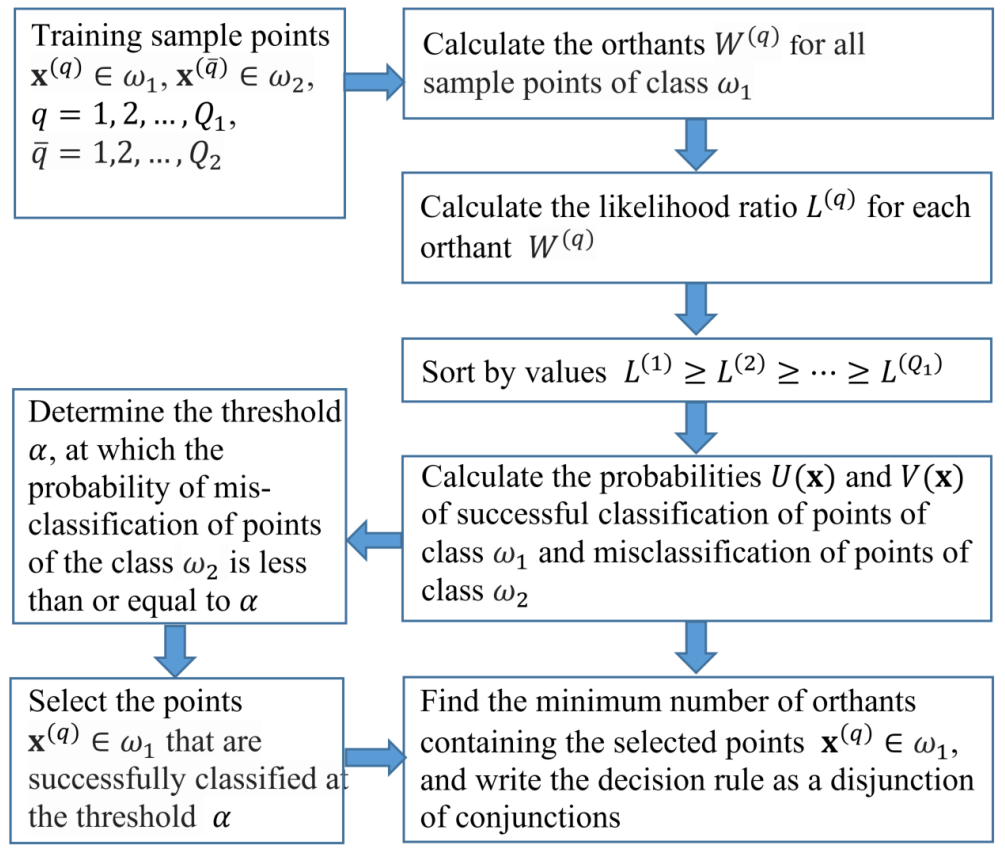
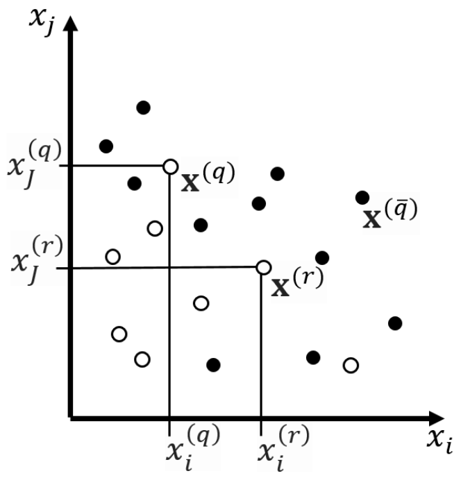
Figure 1 represents the flowchart of the algorithm of the method of monotonic functions. An example of sample points and orthants in the space of two features is shown in Figure 2. The orthants correspond to the decision rule:

IF

$$(x_i\le x_i^{\left(r\right)}\mathbf{AND} x_J\le x_j^{\left(r\right)})\mathbf{OR}(x_i\le x_i^{\left(q\right)}\mathbf{AND} x_J\le x_j^{\left(q\right)})$$

(7)

THEN

the point $\mathbf{x}$ belongs to class ${\omega }_1$ with probability $U\left(\mathbf{x}\right)=7/8$ and with probability $V\left(\mathbf{x}\right)=2/12$ belongs to class ${\omega }_2$.

Due to the increase in the size of the orthants after correction, the probability of a false alarm may increase. If this result is unacceptable, then the number of orthants must be increased. The threshold value $\alpha$ and the number of conjunctions K in the logical function are selected using several iterations.

4. Diagnosis of Indolent and Aggressive Forms of PCa before Treatment

4.1. Data

Studies on the use of pretreatment data in patients with PCa are being conducted to facilitate clinical decisions regarding the type of treatment and to assess the risk of disease recurrence after treatment. According to the results of retrospective studies, preoperative overdiagnosis (when the stage of prostate cancer exposed before surgery is higher than that identified by the final histological conclusion) occurs in 30–45% of cases [21], and underdiagnosis—in 10–15% of cases [22,23]. For this reason, patients with indolent forms of prostate cancer received over-treatment with difficulties in subsequent labor and social rehabilitation and a decrease in the quality of life in general; and in case of preoperative underestimation of the degree of aggressiveness of the tumor process, the volume of primary therapeutic measures, including surgical ones, was insufficient, with a high probability of disease recurrence. Thus, the correct preoperative staging of prostate cancer is one of the most important and urgent tasks of modern urological oncology. To this end, new machine techniques are being developed to improve the preoperative stage of prostate cancer.

To classify patients with indolent and aggressive PCa, we used data from P.A. Hertzen Moscow Research Oncological Institute (Branch of the Federal State Budgetary Institution “National Medical Research Radiological Centre”, Ministry of Health of the Russian Federation). The data sample was taken from the case histories of 341 patients operated on with a diagnosis of PCa: 124 patients with indolent PCa (class ${\omega }_1$) and 217 patients with aggressive PCa (class ${\omega }_2$). The form of prostate cancer was determined by postoperative data.

The preoperative state of the patient is described by the following indicators:

1.

Histological analysis data (needle 12-gauge biopsy). Gleason Group (GrGl) for two characteristic biopsy sites on the Gleason scale [24]. The indicator takes the following values:

• GrGl = 1, if the score is 6 or less;
• GrGl = 2, if the score is 7 = 3 + 4 (the order of the items is important);
• GrGl = 3, if the score is 7 = 4 + 3 (the order of the items is important);
• GrGl = 4, if the score is 8 or higher.

2.

Indicators of immunochemical analysis of blood (Beckman Coulter—Access 2 chemiluminescent analyzer, USA; Hybritech calibration) [25].

• tPSA is a total Prostate-Specific Antigen.
• fPSA is a free PSA.
• [−2]proPSA is a precursor isoform of PSA.
• fPSA/tPSA.
• PHI = $\frac{[-2]\mathrm{proPSA}}{\mathrm{fPSA}}\times \sqrt{\mathrm{tPSA}}$ is the Prostate Health Index.

3.

Indicators of clinical group.

• V is the volume of the prostate according to ultrasound (cm${}^3$).
• Tumor process localization. The indicator takes on the following values:
  • T1 = 1, T2 = 1, if the tumor process is local;
  • T3 = 2, if the tumor process is locally distributed;
  • T4 = 3, there were no cases of T4 in the study population.

4.

Anthropometric indicators.

• Age (years).
• (BMI) = (body mass)/(height)${}^2$ is a Body Mass Index (kg/m${}^2$).

The form of the disease after surgery was determined by two postoperative indicators: clinical stage (GrT) and Gleason Group (GrGl). If, as a result of histological examination, it was found that the prevalence of the primary tumor in the prostate did not exceed T2 (the tumor process was local and there were no metastases to regional lymph nodes and distant metastases) and the Gleason Group was no more than six points, then the cancer status of the prostate was considered indolent. Otherwise, the PCa status was considered aggressive.

4.2. Materials and Methods

The study included only primary patients with a confirmed diagnosis of prostate cancer and a tPSA level $<30$ ng/mL according to the WHO calibration (ARCHITECT i1000SR, Abbott, USA) before surgery. All patients were operated. The average age of patients is $62.6\pm 0.4$ years (41–85 years). Most patients with prostate cancer are persons aged 51–60 years—29.4% and 61–70 years old—53.8%; men under 50 make up 4.7%, under 70—12.2%.

The patient’s preoperative data include: the degree of differentiation of tumor tissue according to the results of biopsy (6–12 points) according to the Gleason scale; laboratory parameters: serum levels of tPSA, fPSA, [−2] proPSA; classification of TNM tumor according to the results of clinical examination; age. After surgery, patients were characterized by pTNM-classification of the tumor process [26], including the assessment of tumor aggressiveness according to the Gleason scale in accordance with the pathomorphological conclusion after prostatectomy.

Before the surgery, the patients were divided into stages T1 (12%—40 patients), T2 (69%—235 patients), T3 (19%—66 patients). After surgery, the T1–T2 stage was insufficient in 31% of cases (in 84 of 275 patients the stage was changed to pT3), T3 became excessive in 26% of cases (in 17 of 66 patients the stage was pT2). After surgery, the dominant group consisted of patients with PCa pT2 (61%), including 56.3% of patients with pT2c. In 133 (39%) patients with prostate cancer, the tumors corresponded to pT3 (pT3a—19.4% and pT3b—19.6%). These data are summarized in

Table 1. Distribution of patients by the volume of prostate tumor lesions by biopsy (T) and after surgery (pT).

T	Before Surgery		After Surgery
	n	%	n	%
T1	40	11.7%	—	—
T2, including:	235	68.9%	208	61.0%
T2a–b	111	32.6%	16	4.7%
T2c	124	36.4%	192	56.3%
T3, including:	66	19.4%	133	39.0%
T3a	37	10.9%	66	19.4%
T3b	29	8.5%	67	19.6%

.

The distribution of prostate cancer patients according to the tumor grade according to the Gleason scale is presented in

Table 2. Distribution of patients by the degree of tumor malignancy according to the Gleason scale in accordance with the final histological conclusion.

Gleason Index	Before Surgery		After Surgery
	n	%	n	%
3	2	0.6%	1	0.3%
4	4	1.2%	3	0.9%
5	33	9.7%	24	7.0%
6	169	49.6%	124	36.4%
7, including:	109	32.0%	159	46.6%
7 (3 + 4)	65	19.1%	95	27.9%
7 (4 + 3)	41	12.0%	51	15.0%
8	17	5.0%	17	5.0%
9	7	2.1%	13	3.8%

. Of the entire sample, according to the histological examination of biopsy material, 208 (61%) patients had highly differentiated prostate cancer (Gleason index up to 6), 109 (32%) patients had a Gleason index of 7, and 24 (7%) patients had a Gleason index 8 or more. According to the results of a pathomorphological study, the proportion of patients with a low Gleason grade of tumor malignancy (with an indicator of up to 6) decreased to 44.6%. Gleason level 7 was recorded in more patients than before surgery—in 46.6% of cases. The smallest was the group with a Gleason score of 8–9 (8.8%). Thus, after surgery, 43.8% of patients (91 out of 208) with a Gleason biopsy score of up to 6 were diagnosed with a high degree of tumor malignancy (≥7), and 5.2% of patients (7 out of 133) had a biopsy of ≥7 showed a low tumor grade (≤6).

The prevalence of the tumor process in the PT of the prostate gland and the degree of its differentiation (Gleason index according to the results of pathological and anatomical examination) were used to divide patients according to the aggressiveness of the tumor process [27,28,29] into the following groups:

• Indolent PCa (124 patients)

  -

  Localized PCa: pT2N0 and Gleason index up to 6

• Aggressive PCa (217 patients)

  -

  Localized prostate cancer: pT2N0 and Gleason score greater than or equal to 7 (85 prostate cancer patients)

  -

  Locally advanced PCa: pT3N0 (87 PCa patients)

  -

  PCa with regional metastases: pT1-3N+ (45 PCa patients).

Serum levels of total PSA (ng/mL), fPSA (ng/mL), [−2]proPSA (pg/mL) were assessed by chemiluminescence using an immunochemical assay system (Access 2, Beckman Coulter, CA, USA) with Hybritech calibration. On their basis, the indicators% fPSA,% [−2] proPSA and PHI were calculated according to the following formulas:

$$\%\mathrm{fPSA}=\frac{\mathrm{fPSA}(\mathrm{ng}/\mathrm{mL})}{\mathrm{tPSA}(\mathrm{ng}/\mathrm{mL})}\ast 100\%$$

$$\%[-2]\mathrm{proPSA}=\frac{[-2]\mathrm{proPSA}(\mathrm{ng}/\mathrm{mL})}{\mathrm{fPSA}(\mathrm{ng}/\mathrm{mL})}\ast 100\%$$

$$\mathrm{PHI}=\frac{[-2]\mathrm{proPSA}}{\mathrm{fPSA}}\times \sqrt{\mathrm{tPSA}}$$

Table 3. Statistical indicators of a sample of patients with indolent (class ${\omega }_1$) and aggressive (class ${\omega }_2$) prostate cancer.

	tPSA	fPSA	ProPSA	PHI	Age	BMI	V	T	GrGl	tPSA/ fPSA
Indolent form (class ${\omega }_1$)
Average	9.13	0.94	17.19	55.57	61.46	28.60	45.11	1.05	1.06	10.85
Standard deviation	5.49	0.69	12.72	26.67	6.48	17.78	25.14	0.21	0.23	4.75
Aggressive form (class ${\omega }_2$)
Average	13.94	1.17	26.76	84.61	63.44	26.90	38.87	1.29	2.01	12.70
Standard deviation	8.29	0.72	19.95	46.29	6.83	5.66	15.31	0.45	1.04	5.81

presents statistics for a sample of patients. It can be seen that some indicators poorly distinguish between patients by disease forms.

4.3. Modeling and Results

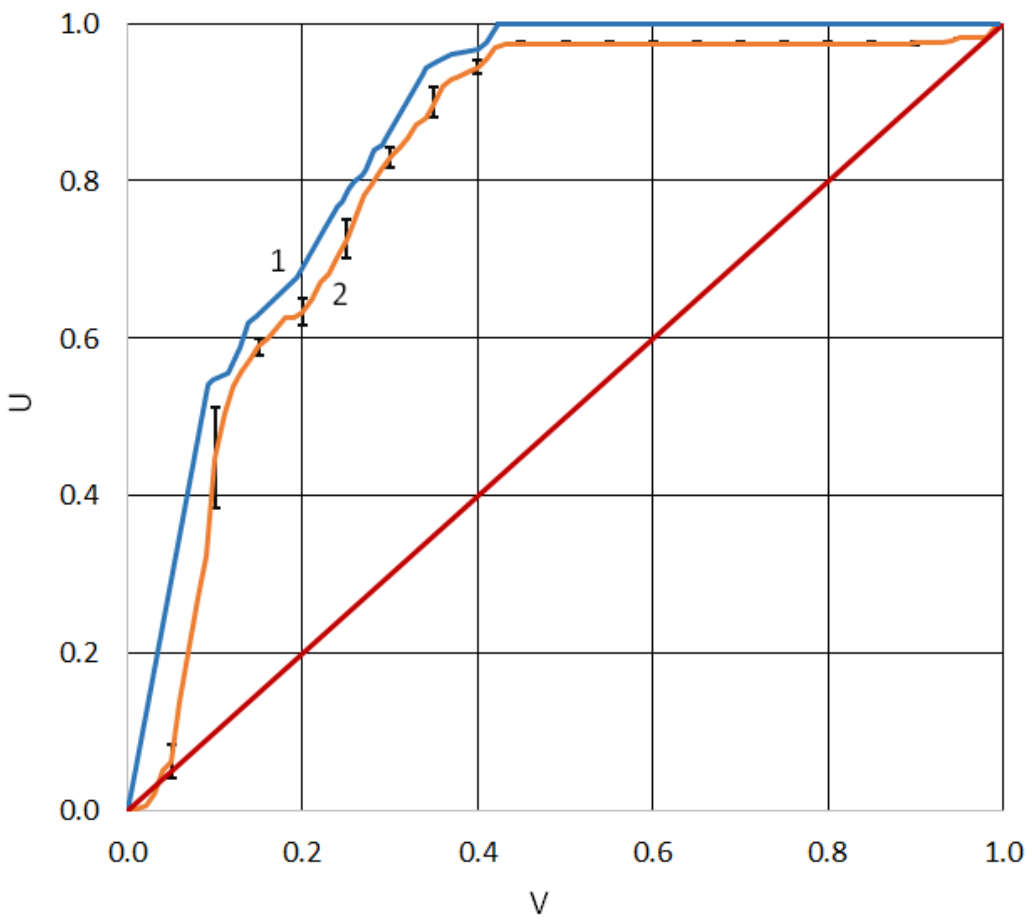
The classification rule was sought using the algorithm of the method of monotonic functions. The software implementation of the algorithm includes a step-by-step feature selection technique and a cross-validation method to assess the quality of the classification. The best classification results were obtained according to the following three indicators: GrT, GrGl, and tPSA. Dependences $U\left(V\right)$ of the probability of successful detection of patients with the indolent form of the disease $U\left(\mathbf{x}\right)$ on the probability of misclassification of patients with an aggressive form of the disease $V\left(\mathbf{x}\right)$ (probability of false alarm) are presented in Figure 3, where line 1 shows the dependence $U\left(V\right)$ when tested on the training set, and line 2 shows the dependence $U\left(V\right)$ averaged over 10 tests using k-fold cross-validation at $k=10$. The vertical segments in Figure 1 indicate the values of the standard deviations.

Notably, the classification results differed little when tPSA was replaced with PHI or fPSA/tPSA. Adding other features to the selected set of indicators significantly increased the discrepancy between the test results for the training set and the test results using cross-validation. In this case, the result of the test of the classification rule for the training set significantly improved, and the result of the cross-validation test slightly worsened. Therefore, such options for solving the problem were not considered.

Figure 3 shows that the results of testing the classification rule based on the training sample and cross-validation are very close. Therefore, to explain the decision, it is permissible to use logical rules obtained from the training sample. The $U\left(V\right)$ dependence determines the threshold that provides the same decision-making efficiency when classifying patients with indolent and aggressive PCa [30,31]. For this threshold, the decision on the training sample (line 1) corresponds to the probability of the successful classification of patients with indolent PCa $U\left(\mathbf{x}\right)=0.765$ and the probability of misclassification of patients with aggressive PCa $V\left(\mathbf{x}\right)=0.235$.

The threshold $\alpha =0.235$ corresponds to the rule:

IF

$$\begin{array}{cccccc}\hfill & (\mathrm{tPSA}\le 9.72)& \mathbf{AND}\hfill & (\mathrm{GrGl}=1)& & \\ \hfill \mathbf{OR}& (\mathrm{tPSA}\le 8.24)& \mathbf{AND}\hfill & (\mathrm{GrGl}\le 2)& \mathbf{AND}& (\mathrm{GrT}=1)\\ \hfill \mathbf{OR}& (\mathrm{tPSA}\le 11.39)& \mathbf{AND}\hfill & (\mathrm{GrGl}=1)& \mathbf{AND}& (\mathrm{GrT}=1)\end{array}$$

(8)

THEN

the patient has indolent PCa with a probability$U\left(\mathbf{x}\right)=0.765$and with the probability of misclassification of a patient with aggressive PCa,$V\left(\mathbf{x}\right)=0.235$.

If this condition is not met, then the patient has aggressive PCa with a probability of $1-V\left(\mathbf{x}\right)=0.765$, whereas the probability of misclassification of a patient with indolent PCa is $1-U\left(\mathbf{x}\right)=0.235$.

Below, we provide several examples of the found classification rule for the thresholds $\alpha =0.10$, $\alpha =0.15$, $\beta =0.90$, and $\beta =0.85$.

The threshold $\alpha =0.10$ corresponds to the rule:

IF

$$\begin{array}{cccccc}\hfill & (\mathrm{tPSA}\le 8.21)& \mathbf{AND}\hfill & (\mathrm{GrGl}=1)& & \\ \hfill \mathbf{OR}& (\mathrm{tPSA}\le 8.40)& \mathbf{AND}\hfill & (\mathrm{GrGl}=1)& \mathbf{AND}& (\mathrm{GrT}=1)\end{array}$$

(9)

THEN

the patient has indolent PCa with a probability$U\left({\omega }_1\right)=0.548$and with the probability of misclassification of a patient with aggressive PCa,$V\left({\omega }_1\right)=0.097$.

The threshold $\alpha =0.15$ corresponds to the rule:

IF

$$\begin{array}{cccccc}\hfill & (\mathrm{tPSA}\le 9.72)& \mathbf{AND}\hfill & (\mathrm{GrGl}=1)& & \\ \hfill \mathbf{OR}& (\mathrm{tPSA}\le 10.06)& \mathbf{AND}\hfill & (\mathrm{GrGl}=1)& \mathbf{AND}& (\mathrm{GrT}=1)\end{array}$$

(10)

THEN

the patient has indolent PCa with a probability$U\left({\omega }_1\right)=0.629$and with the probability of misclassification of a patient with aggressive PCa,$V\left({\omega }_1\right)=0.147$.

The threshold $\beta =0.90$ corresponds to the rule:

IF the following condition is not fulfilled:

$$\begin{array}{cccccc}\hfill & (\mathrm{tPSA}\le 9.72)& \mathbf{AND}\hfill & (\mathrm{GrGl}=1)& & \\ \hfill \mathbf{OR}& (\mathrm{tPSA}\le 8.24)& \mathbf{AND}\hfill & (\mathrm{GrGl}\le 2)& \mathbf{AND}& (\mathrm{GrT}=1)\\ \hfill \mathbf{OR}& (\mathrm{tPSA}\le 19.09)& \mathbf{AND}\hfill & (\mathrm{GrGl}=1)& \mathbf{AND}& (\mathrm{GrT}=1)\end{array}$$

(11)

THEN

the patient has aggressive PCa with a probability$1-V\left({\omega }_1\right)=0.659$and with the probability of misclassification of a patient with indolent PCa, $1-U\left({\omega }_1\right)=0.057$.

The threshold $\beta =0.85$ corresponds to the rule:

IF the following condition is not fulfilled:

$$\begin{array}{cccccc}\hfill & (\mathrm{tPSA}\le 9.72)& \mathbf{AND}\hfill & (\mathrm{GrGl}=1)& & \\ \hfill \mathbf{OR}& (\mathrm{tPSA}\le 8.24)& \mathbf{AND}\hfill & (\mathrm{GrGl}\le 2)& \mathbf{AND}& (\mathrm{GrT}=1)\\ \hfill \mathbf{OR}& (\mathrm{tPSA}\le 13.96)& \mathbf{AND}\hfill & (\mathrm{GrGl}=1)& \mathbf{AND}& (\mathrm{GrT}=1)\end{array}$$

(12)

THEN

the patient has aggressive PCa with a probability$1-V\left({\omega }_1\right)=0.719$and with the probability of misclassification of a patient with indolent PCa,$1-U\left({\omega }_1\right)=0.161$.

5. Conclusions

The method of monotonic functions is intended for solving problems of binary classification with ordered classes. The method of solution assumes that the decision rule is associated with the ordinal number of the class by a monotonic non-decreasing function of indicators of the patient’s condition (from the features of classification). In a simplified formulation, the method classifies the belonging of an object to the first class ${\omega }_1$ if all the attributes of the object are less than or equal to the values of the attributes of any object in the training set of this class. If the value of at least one feature of the object is greater than the corresponding value of the object of the training sample of the first class, then a decision is made on the belonging of such an object to the second class ${\omega }_2$. The monotonicity condition makes it possible to compare patients according to the severity of the disease. Indeed, if all the key indicators in the observed patient are closer to the normal indicators of a healthy person than in a control patient with a known severity of the disease, then it is quite natural to consider the condition of this patient to be easier. On the other hand, if at least one of the key indicators of the observed patient is further from the norm than that of the control patient, then the patient’s condition is more severe.

Machine classification methods find rules that generalize objects within classes and separate objects of different classes. In the feature space, each patient q corresponds to a vector ${\mathbf{x}}^{\left(q\right)}$, the components of which are the patient’s indicators. During training, the vector ${\mathbf{x}}^{\left(q\right)}$ of the class ${\omega }_1$ of patients with indolent prostate cancer selects a set of vectors that correspond to patients with similar indicators. The monotonicity condition is that this set is an orthant, which contains only vectors with values of indicators no more than y for a patient q. This set can include vectors not only of class ${\omega }_1$, but also of class ${\omega }_2$. The larger the fraction of vectors of the class ${\omega }_1$, the better this orthant separates the classes. The learning algorithm selects the orthants with the best measure of separability. This allows us to find a classification rule that, in the training sample, provides a close to maximum probability of successful classification of patients with indolent PCa (class ${\omega }_1$), provided the probability of misclassification of patients with aggressive PCa (class ${\omega }_2$) is given.

When teaching, the method extracts empirical knowledge that explains the result of the classification. The justification of the result by analogy with the precedent is as follows. The decision rule for a new patient, to whom the vector $\mathbf{x}$ corresponds, finds all orthants of the training sample that contain the vector $\mathbf{x}$. This is tantamount to selecting from the training sample a set of patients with an indolent form of the disease, in whom all the values of the indicators differ from the norm more than in the subject. If the monotonic condition is correct, follow the principle of analogy, this patient has an indolent form of the disease. If there are no orthants containing the vector $\mathbf{x}$ in the training set, then a decision is made for this patient about the aggressive form of the disease.

Obviously, the probability of the vector $\mathbf{x}$ falling into the orthant is the less, the smaller the number of vectors of the class ${\omega }_1$ got into this orthant during training. This pattern is manifested in the fact that the probability of successful classification of patients in the training sample can be significantly higher than the probability of classifying patients on the test sample and when modeling the test sample using the cross-validation procedure. It is well known that, in the general case, the number of vectors in orthants will decrease with an increase in the number of indicators used in the classification rule. This reduces the generalizing ability of the method. To overcome this drawback, it is necessary to increase the number of patients in the training sample with an increase in the number of indicators.

The second justification of the classification result is performed using a logical function. Each connection of the decision rule corresponds to an orthant, which is determined by the parameters of a patient with an indolent form of the disease (class ${\omega }_1$). Logical rules (8)–(12) consist of 2–3 conjunctions, which in the learning process are selected from 124 conjunctions of the training sample. Each of the conjunctions participating in the above rules corresponds to an orthant containing a sufficiently large number of vectors of the class ${\omega }_1$. Thus, each logical rule (8)–(12) generalizes well enough the knowledge contained in the training sample of patients. Therefore, solution (8) gives a rule that determines the balance point between sensitivity and specificity. When (8) is fulfilled, the probability of successful classification of patients with indolent form is $U\left(\mathbf{x}\right)=0.765$ with the probability of misclassification of patients with aggressive form $V\left(\mathbf{x}\right)=0.235$. If this rule is not met, then we obtain a solution at which the probability of correct classification of patients with an aggressive form of $1-V\left(\mathbf{x}\right)=0.765$ with an erroneous classification of patients with an indolent form of $1-U\left(\mathbf{x}\right)=0.235$. Equations (9)–(12) give higher levels of probability of successful classification for patient subgroups.

The data of 341 case histories of operated patients with indolent and aggressive forms of prostate cancer were analyzed. Analysis of preoperative and postoperative data revealed the dependence of the form of prostate cancer on preoperative data. This relationship is used to classify the form of the disease. For this, it is required to indicate to the algorithm either the threshold value of the probability of successful classification of patients with an indolent form of the disease or the threshold value of the probability of misclassification of patients with an aggressive form of the disease.

As a result, we can draw two conclusions about the application of the method of monotonic functions to the problem of classifying the form of prostate cancer according to the data before treatment: (1) The satisfactory quality of the solution allows us to consider the uniformity model. as adequate to the problem being solved; (2) The above examples (8)–(12) show that the calculated logical rules are quite simple and easily interpreted from the point of view of preoperative indicators of the form of the disease.

References

- Fatima, M.; Pasha, M. Survey of Machine Learning Algorithms for Disease Diagnostic. J. Intell. Learn. Syst. Appl. 2017, 9, 73781. [Google Scholar] [CrossRef]
- Rajkomar, A.; Dean, J.; Kohane, I. Machine learning in medicine. N. Engl. J. Med. 2019, 380, 1347–1358. [Google Scholar] [CrossRef]
- Alkhateeb, A.; Atikukke, G.; Rueda, L. Machine learning methods for prostate cancer diagnosis. J. Cancer 2020, 3, 70–75. [Google Scholar]
- Stephan, C.; Kahrs, A.; Cammann, H.; Lein, M.; Schrader, M.; Deger, S.; Miller, K.; Jung, K. A [−2] proPSA-based artificial neural network significantly improves differentiation between prostate cancer and benign prostatic diseases. Prostate 2009, 69, 198–207. [Google Scholar] [CrossRef] [PubMed]
- Vinitskaia, R.; Gitis, V.; Eramian, S.; Nagornov, V.; Sungurian, N. Possibilities of determination of quantitative relationship between the evaluation of clinical condition and functional signs of respiratory insufficiency with the aid of mathematical methods. Zhurnal Eksperimental’noi Klin. Meditsiny 1977, 17, 113–121. [Google Scholar]
- Turbovich, I.; Vinitskaia, R.; Gitis, V.; Nagornov, V.; Eramian, S.; Nagornov, V.; Eramian, S.; Sungurian, N. Analysis of the relationship between the severity of the patient’s condition and his physiological indicators in Pattern Recognition. Zhurnal Eksperimental’noi Klin. Meditsiny 1977, 5, 22–26. [Google Scholar]
- Rawla, P. Epidemiology of prostate cancer. World J. Oncol. 2019, 10, 63–89. [Google Scholar] [CrossRef] [PubMed]
- Partin, A.; Brawer, M.; Bartsch, G.; Horninger, W.; Taneja, S.; Lepor, H.; Babaian, R.; Childs, S.; Stamey, T.; Fritsche, H.; et al. Complexed prostate specific antigen improves specificity for prostate cancer detection: Results of a prospective multicenter clinical trial. J. Urol. 2003, 170, 1787–1791. [Google Scholar] [CrossRef]
- Jansen, F.; van Schaik, R.; Kurstjens, J.; Horninger, W.; Klocker, H.; Bektic, J.; Wildhagen, M.; Roobol, M.; Bangma, C.; Bartsch, G. Prostate-specific antigen (PSA) isoform p2PSA in combination with total PSA and free PSA improves diagnostic accuracy in prostate cancer detection. Eur. Urol. 2010, 57, 921–927. [Google Scholar] [CrossRef]
- Catalona, W.; Partin, A.; Sanda, M.; Wei, J.; Klee, G.; Bangma, C.; Slawin, K.; Marks, L.; Loeb, S.; Broyles, D.; et al. A multi-center study of [−2] pro-prostate-specific antigen (PSA) in combination with PSA and free PSA for prostate cancer detection in the 2.0 to 10.0 ng/mL PSA range. J. Urol. 2011, 185, 1650–1655. [Google Scholar] [CrossRef]
- Cooperberg, M.R.; Pasta, D.J.; Elkin, E.P.; Litwin, M.S.; Latini, D.M.; Du Chane, J.; Carroll, P.R. The University of California, San Francisco Cancer of the Prostate Risk Assessment score: A straightforward and reliable preoperative predictor of disease recurrence after radical prostatectomy. J. Urol. 2005, 173, 1938–1942. [Google Scholar] [CrossRef]
- Cooperberg, M.R.; Hilton, J.F.; Carroll, P.R. The CAPRA-S score: A straightforward tool for improved prediction of outcomes after radical prostatectomy. Cancer 2011, 117, 5039–5046. [Google Scholar] [CrossRef]
- Lorent, M.; Maalmi, H.; Tessier, P.; Supiot, S.; Dantan, E.; Foucher, Y. Meta-analysis of predictive models to assess the clinical validity and utility for patient-centered medical decision making: Application to the CAncer of the Prostate Risk Assessment (CAPRA). BMC Med. Inform. Decis. Mak. 2019, 19, 2. [Google Scholar] [CrossRef]
- Mamidi, Y. Classification of Prostate Cancer Patients into Indolent and Aggressive Using Machine Learning. Master’s Thesis, University of New Orleans, New Orleans, LA, USA, 2020. [Google Scholar]
- Sergeeva, N.; Skachkova, T.; Alekseev, B.Y.; Yurkov, E.; Pirogov, S.; Gitis, V.; Marshutina, N.; Kaprin, A. APHIG: A new multiparameter index for prostate cancer. Cancer Urol. 2016, 12, 94–103. [Google Scholar] [CrossRef][Green Version]
- Sergeeva, N.; Skachkova, T.; Marshutina, N.; Nyushko, K.; Shevchuk, I.; Nazirov, M.; Alekseev, B.; Pirogov, S.; Yurkov, E.; Gitis, V.; et al. The validation of threshold decision rules and calculator for APhiG algoritm for clarification of prostate cancer staging before treatment. Cancer Urol. 2020, 16, 43–53. [Google Scholar] [CrossRef]
- Yurkov, E.; Pirogov, S.; Gitis, V.; Sergeeva, N.; Alekseev, B.Y.; Skachkova, T.; Kaprin, A. Prediction of the Aggressive Status of Prostate Cancer on the Basis of Preoperative Data. J. Commun. Technol. Electron. 2017, 62, 1448–1455. [Google Scholar] [CrossRef]
- Yurkov, E.; Pirogov, S.; Gitis, V.; Sergeeva, N.; Skachkova, T.; Alekseev, B.Y.; Kaprin, A. Diagnostic Model that Takes Medical Preferences into Account. Prediction of the Clinical Status of Prostate Cancer. J. Commun. Technol. Electron. 2019, 64, 834–845. [Google Scholar] [CrossRef]
- Alekseev, B.; Skachkova, T.; Sergeeva, N.; Pirogov, S.; Gitis, V.; Yurkov, E.; Kaprin, A. New algorithm aphigt for prostate cancer staging: MP53-09. J. Urol. 2018, 199, e707. [Google Scholar] [CrossRef]
- Zakrevskii, A. “Optimization of coverings of sets”. In Logical Language for Representation of Synthesis Algorithms of Relay Devices; Zakrevskii, A., Ed.; Nauka: Moscow, Russia, 1966; pp. 136–147. [Google Scholar]
- Sardana, G.; Dowell, B.; Diamandis, E. Emerging biomarkers for the diagnosis and prognosis of prostate cancer. Clin. Chem. 2008, 54, 1951–1960. [Google Scholar] [CrossRef] [PubMed]
- Postma, R.; Schröder, F. Screening for prostate cancer. Eur. J. Cancer 2005, 41, 825–833. [Google Scholar] [CrossRef]
- Schröder, F.; Hugosson, J.; Roobol, M.; Tammela, T.; Ciatto, S.; Nelen, V.; Kwiatkowski, M.; Lujan, M.; Lilja, H.; Zappa, M.; et al. Prostate-cancer mortality at 11 years of follow-up. N. Engl. J. Med. 2012, 366, 981–990. [Google Scholar] [CrossRef] [PubMed]
- Hsieh, T.F.; Chang, C.H.; Chen, W.C.; Chou, C.L.; Chen, C.C.; Wu, H.C. Correlation of Gleason scores between needle-core biopsy and radical prostatectomy specimens in patients with prostate cancer. J. Chin. Med. Assoc. 2005, 68, 167–171. [Google Scholar] [CrossRef]
- Stephan, C.; Kahrs, A.M.; Klotzek, S.; Reiche, J.; Müller, C.; Lein, M.; Deger, S.; Miller, K.; Jung, K. Toward metrological traceability in the determination of prostate-specific antigen (PSA): Calibrating Beckman Coulter Hybritech Access PSA assays to WHO standards compared with the traditional Hybritech standards. Clin. Chem. Lab. Med. (CCLM) 2008, 46, 623–629. [Google Scholar] [CrossRef] [PubMed]
- Sobin, L.H.; Gospodarowicz, M.K.; Wittekind, C. TNM Classification of Malignant Tumours; John Wiley & Sons: Hoboken, NJ, USA, 2011. [Google Scholar]
- Cantiello, F.; Russo, G.; Cicione, A.; Ferro, M.; Cimino, S.; Favilla, V.; Perdonà, S.; De Cobelli, O.; Magno, C.; Morgia, G.; et al. PHI and PCA3 improve the prognostic performance of PRIAS and Epstein criteria in predicting insignificant prostate cancer in men eligible for active surveillance. World J. Urol. 2016, 34, 485–493. [Google Scholar] [CrossRef]
- Kryvenko, O.; Carter, B.; Trock, B.; Epstein, J. Biopsy criteria for determining appropriateness for active surveillance in the modern era. Urology 2014, 83, 869–874. [Google Scholar] [CrossRef]
- Han, J.; Toll, A.; Amin, A.; Carter, B.; Landis, P.; Lee, S.; Epstein, J. Low prostate-specific antigen and no Gleason score upgrade despite more extensive cancer during active surveillance predicts insignificant prostate cancer at radical prostatectomy. Urology 2012, 80, 883–888. [Google Scholar] [CrossRef][Green Version]
- Metz, C.E. Basic principles of ROC analysis. Semin. Nucl. Med. 1978, 8, 283–298. [Google Scholar] [CrossRef]
- Kim, D.S.; McCabe, C.J.; Yamasaki, B.L.; Louie, K.A.; King, K.M. Detecting random responders with infrequency scales using an error-balancing threshold. Behav. Res. Methods 2018, 50, 1960–1970. [Google Scholar] [CrossRef]