Abstract
Maize straw is a valuable renewable energy source. The rapid and accurate determination of its yield and spatial distribution can promote improved utilization. At present, traditional straw estimation methods primarily rely on statistical analysis that may be inaccurate. In this study, the Gaofen 6 (GF-6) satellite, which combines high resolution and wide field of view (WFV) imaging characteristics, was used as the information source, and the quantity of maize straw resources and spatial distribution characteristics in Qihe County were analyzed. According to the phenological characteristics of the study area, seven classification classes were determined, including maize, buildings, woodlands, wastelands, water, roads, and other crops, to explore the influence of sample separation and test the responsiveness to different land cover types with different waveband combinations. Two supervised classification methods, support vector machine (SVM) and random forest (RF), were used to classify the study area, and the influence of the newly added band of GF-6 WFV on the classification accuracy of the study area was analyzed. Furthermore, combined with field surveys and agricultural census data, a method for estimating the quantity of maize straw and analyzing the spatial distribution based on a single-temporal remote sensing image and random forests was proposed. Finally, the accuracy of the measurement results is evaluated at the county level. The results showed that the RF model made better use of the newly added bands of GF-6 WFV and improved the accuracy of classification, compared with the SVM model; the two red-edge bands improved the accuracy of crop classification and recognition; the purple and yellow bands identified non-vegetation more effectively than vegetation, thus minimizing the “salt-and-pepper noise” of classification results. However, the changes to total classification accuracy were not obvious; the theoretical quantity of maize straw in Qihe County in 2018 was 586.08 kt, which reflects an error of only 2.42% compared to the statistical result. Hence, the RF model based on single-temporal GF-6 WFV can effectively estimate regional maize straw yield and spatial distribution, which lays a theoretical foundation for straw recycling.
1. Introduction
China is a large country known for its abundant agricultural resources, with agricultural production comprising a significant proportion of its national economy [1]. Crop straw, as a by-product of agricultural production [2], is an indispensable production material in vast rural areas [3]. In recent years, as the rural energy structure has shifted, fewer people have used straw as an energy resource for rural life because of its large volume and scattered distribution, as well as the low degree of industrialization [4]. Furthermore, owing to the regional, seasonal, and structural surplus of straw becoming increasingly prominent, a large amount of straw is still not fully utilized, which severely restricts the development of circular agriculture in China [5,6]. Although the government advocates for the return of straw to the field [7], straw is often discarded or burned in large amounts to allow for timely sowing at the start of the growing season, leading to the serious waste of resources and environmental pollution [8]. Straw is beneficial if used, but it is harmful if it is discarded [9]. With the development of renewable energy technology, biotechnology, circular agriculture, and environmental science, the value of crop straw as a renewable energy source has gradually been increasing and become widely accepted [10], which can be used as bio-fertilizer, feed, raw materials, fuels, and base materials. Therefore, studying the quantity and spatial distribution of straw resources in China and promoting the comprehensive utilization of straw resources are necessary for promoting rural building and sustainable agricultural development in China [11].
Although the current straw quantity was estimated in many studies, there are several limitations to extant methods and findings [12]. Firstly, the low resolution of statistical data is generally used for the analysis of straw at the county level or above, which limits the value of the data for detailed spatial analyses [13]. Secondly, the quantity of straw resources cannot be calculated in time, because the agricultural census can only be completed in the next year at the earliest. Moreover, if we aim to realize the comprehensive utilization of straw, we must not only estimate the straw yield but also fully consider the spatial distribution of regional straw [14]. The effective recycling and utilization of crop straw resources can be realized more efficiently by combining the relationship between the supply and demand of regional straw resources and optimizing straw recycling and comprehensive utilization [15].
With the in-depth application of remote sensing technology in crop area extraction, growth monitoring [16], and yield estimation [17], the use of remote sensing technology to analyze the yield and spatial distribution of straw has become a major development direction for straw resource investigation [18]. The spatial characteristics of crop planting in China exhibit complex structures and fragmentations. Therefore, in the estimation of large-scale straw quantity, the data to be processed are very large when the high-resolution remote sensing image is used, while the low-resolution remote sensing image will lead to a rapid decline in the measurement accuracy [19]. Classification using single-temporal remote sensing images of the “key phenological period” combined with multi-characteristic parameters and sensitive bands has become an important method for current crop type identification [20]. The response characteristics of different wavebands to different crops can be used to optimize the combination of wavebands, so that the spectral difference and Class Separability between different crop types are significantly improved, and finally, the accurate investigation and analysis of different crop straw resources can be realized [21].
Maize, which accounts for approximately one-fifth of grain crops in China, is the third-largest grain crop after rice and wheat [22]. Therefore, the quantity and spatial distribution of maize straw in the region are of great significance to the collection, storage, and transportation as well as comprehensive utilization of straw.
The Gaofen-6 (GF-6) satellite, planned in China’s high-resolution major special series satellites, adds four bands with central wavelengths of 710 nm, 750 nm, 425 nm, and 610 nm, which can provide richer spectral information for agricultural research [23]. This technological advancement is important for improving the spectral information characteristics of China’s medium and high-resolution satellites [24].
In order to improve the comprehensive utilization and accelerate the development of the scale, industrialization, and commercialization of straw, the quantity and spatial distribution of straw need to be studied, to plan the recycling network and the site selection of the utilization factory of straw. In this study, the effects of different wavebands on the classification of different land cover types were analyzed based on GF-6 satellite imagery, and the quantity and spatial distribution characteristics of maize straw in Qihe County were estimated to provide data support for recycling and effective utilization of regional straw. The research contents included: (1) exploring and analyzing the impact of different band combinations on samples separability, (2) analyzing the classification accuracy of the support vector machine (SVM) and random forest (RF) classification models under different band combinations for different land cover types, and (3) proposing a method for estimating the quantity and spatial distribution of maize straw based on planting area.
2. Materials and Methods
2.1. Research Area
The study area is located in Qihe County, which is in the southernmost part of Dezhou City, Shandong Province, China, at latitude range 36°24′37″–37°1′44″ N and longitude range 116°23′28″–116°57′35″ E (Figure 1). The annual average temperature is 15 °C throughout the year, which indicates a warm temperate and sub-humid monsoon climate zone, with four distinct seasons and mild weather patterns. The land area of the study area is approximately 1411 km2, of which arable land comprises 840 km2. It is flat, with an average elevation of 26 m (mean sea level), and is an alluvial plain in the lower reaches of the Yellow River. It is also an important food production area in Shandong Province. The main food crops are winter wheat and maize; peanuts, soybeans, and cotton are also planted.
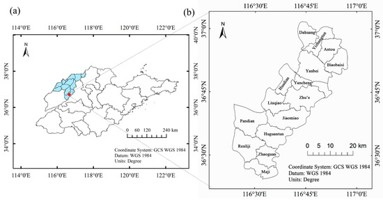
Figure 1.
Research area: (a) Shandong Province; (b) Qihe County.
2.2. Data Source and Preprocessing
The GF-6 was successfully launched on 2 June 2018, and is mainly used in precision agriculture observation and forestry resource investigation. An 8-band complementary metal-oxide-semiconductor detector was employed in China, equipped with a 2 m panchromatic/8 m multi-spectral high-resolution camera and a 16 m multi-spectral medium-resolution wide field of view (WFV) camera. The details of GF6-WFV are shown in Table 1. For the first time in China, the “red-edge” band, which can effectively reflect the unique spectral characteristics of crops, was added, which has greatly improved the monitoring of agriculture, forestry, grassland, and other resources.

Table 1.
Parameters of Gaofen 6 (GF-6) wide field of view (WFV).
The image of the research area taken on 9 September 2018, was selected for analysis, as this date corresponds to the maize filling period. The 1A-level image downloaded from the China Centre for Resources Satellite Data and Application (CCRSDA) (http://www.cresda.com/CN/index.shtml (accessed on 7 February 2020)) must be preprocessed by radiometric calibration, atmospheric correction, and orthorectification [25], and all preprocessing performed in ENVI (Version 5.3, Research System Inc., Boulder, CO, USA). Atmospheric correction was performed using the fast line-of-sight atmospheric analysis of the spectral hypercubes model [26], and the spectral response function was provided by the CCRSDA. The rational polynomial coefficients model based on rational functions was used to further orthorectify without control points. The 2019 agricultural census data including planting area and yields of maize were obtained from the local government website (http://dztj.dezhou.gov.cn/n3100530/n3100065/index.html (accessed on 27 April 2020)), and the administrative boundary vector data of the study area were downloaded from Resource and Environmental Science and Data Center (http://www.resdc.cn/data.aspx?DATAID=202 (accessed on 7 February 2020)). SuperMap (iDEesktop 8C, SuperMap Software Co., Ltd., Beijing, China) was used to process these data and transform the coordinate system. All spatial data were converted into the universal transverse Mercator (WGS84 UTM 45N) projection.
Two types of samples were used in this study, namely training and verification samples, most of which were obtained through ground surveys using OvitalMap (V8.7.1, Beijing Ovital Software Co., Ltd., Beijing, China) in June 2018. In addition, with the support of higher spatial resolution image data, historical data, and expert knowledge, we also acquired a portion of training samples through manual visual interpretation. A total of 689 samples were acquired in this study, including maize, buildings, woodlands, wastelands, water, roads, and other crops. According to the proportions of different land cover types, 250 samples were randomly selected as verification samples and the rest were used for training samples. The training samples were used to classify land cover types in the research area. The supervised classification method was used to obtain the planting area of maize, from which the yield and distribution of maize straw were estimated. The verification sample was used to evaluate the classification accuracy of different land cover types. All samples were randomly collected to cover the entire study area as much as possible and they were quadrats of single crops to better avoid noise and ensure classification accuracy.
When the maize was being harvested in October 2018, three quadrats of 5 m × 10 m were selected in the southern, central, and northern regions of Qihe County, respectively, to count the number of the maize planted and the weight of straw (15% moisture content). These data will be used for the estimation of maize straw yield.
2.3. Classification of Land Cover Types Using Different Bands Combinations
The maize in the research area of the acquired image was in the grain-filling stage, and the main land cover types were determined by ground investigation as maize, buildings, wasteland, water, woodland, roads, vegetables, cotton, and soybean. Soybean and cotton were planted less than the other crops, and their spectral characteristics were similar to those of vegetables. Hence, vegetables, cotton, soybeans, and a very small number of other crops were classified as other crop types, and the identification and statistics of maize were the focus of classification in this study. In summary, we divided the study area into seven final land cover types, including maize, buildings, woodland, wasteland, water, roads, and other crops. Firstly, layer stacking was performed on the preprocessed image, and five schemes (Table 2) were designed for the newly added bands for experimentation. Second, two types of machine learning—SVM [27] and RF [28]—were used to classify the research area [29]. Finally, the classification results of the two classification methods were analyzed on the influence of the red-edge, purple, and blue bands on the recognition of various land cover types to verify the improvement of the classification accuracy of the newly added band of GF-6 WFV compared to GF1/WFV.
Table 2.
Classification schemes with different band combinations.
SVM is based on a statistical learning theory, trying to find an optimal hyperplane as a decision function in high-dimensional space. The number of free parameters used in the SVM does not depend on the number of input features, and the reduction in the number of features is not required to avoid overfitting. SVM provides a generic mechanism to fit the surface of the hyperplane to the data through the use of a kernel function, such as linear, polynomial, or sigmoid curve. RF is a combination of tree predictors which exhibits superior performance in cases with noise and weak discrimination data and is insensitive to the initialization of parameters [30]. Compared to SVM, the number of user-defined parameters in RF is less than the number required for SVMs and easier to define. In this paper, the training of SVM with a linear kernel was performed. ENMAP-BOX [31] was used for RF classification.
2.4. Classes Separability Assessment
Class separability, which is a measure of similarity between classes, can be determined from these values. There are four widely used quantitative measures for class separability: divergence, transformed divergence (TD), Bhattacharyya distance, and Jeffries–Matusita distance (JM) [32]. Divergence is one of the most popular separability measures used in remote sensing, which can be calculated by the mean and variance-covariance matrices of the data representing feature classes. The TD is the standardized form of divergence, which can minimize the effect of several well-separated classes that may increase the average divergence value and make the divergence measure misleading. The Bhattacharyya distance and the JM can be used to estimating the probability of correct classification, and the JM can suppress high separability values by transforming the Bhattacharyya distance values to a specific range.
2.5. Maize Straw Estimation
The goal of county-level straw estimation was to determine the type and quantity of straw resources. The total theoretical quantity of straw was considered the maximum quantity that can be produced in a certain area each year [33]. This value was estimated by taking the crop planting area and straw resource density, and the equation used is as follows:
where: PT is the theoretical total quantity of straw (t); i is the number of different crop straws, and the maize straw was counted in this study, thus, i = 1; Di indicates the straw resource density of the ith crop (t/km2), and Ai is the plantation area of the ith crop (km2).
where: j is a different sampling region; Ci j is the theoretical total quantity of straw resources of the ith crop in area j (kg); Si j is the plantation area of ith crop in area j (m2).
2.6. Accuracy Verification
A confusion matrix [34] was used to evaluate the accuracy of the classification results based on the verification samples of the ground survey. The evaluation indicators include overall accuracy (OA), user accuracy (UA), production accuracy (PA), and kappa coefficient (KC). The OA and KC reflect the overall classification effect, while the PA and UA represent omission and misclassification errors, respectively. Since accuracy is not necessarily normally distributed, the non-parametric Wilcoxon test for paired samples was conducted to evaluate the changes in OA and PA of each land cover type between different bands combination. Besides, the planting area of maize can also be verified by statistical census data.
According to the yield of maize and the straw-grain ratio, the straw yield of maize could be calculated; that is, the theoretical total quantity of maize straw used as validation data was the product of maize yield and straw-grain ratio, and the maize yield was obtained using annual census data [35].
3. Results and Discussion
3.1. Band Reflectivity Analysis
All training samples (179, 68, 50, 19, 28, 49, and 46 samples of maize, buildings, woodlands, wastelands, water, roads, and other crops) were used to perform pixel information statistics for different feature types, and reflectivity curves of different land cover types were drawn, as shown in Figure 2. Vegetation and non-vegetation have significant differences in spectral characteristics. We found that buildings, roads, and wasteland exhibit higher reflectivity in visible wavelengths (B1–B3 and B7–B8), and buildings and other land cover types were strongly separated. Roads and wasteland were significantly different in B4–B6, which can be easily distinguished. Water exhibits strong NIR waves absorption, so the reflectance of water in B4 is lower than that of all other land cover types [36]. Maize, woodland, and other plants exhibit low reflectivity of visible wavelengths due to the absorption of chlorophyll, and their spectral characteristics are similar [37]. Thus, it is difficult to distinguish each plan type, although the reflectivity is higher in B4 (NIR) and B6 (Red-edge 2). In B4, the reflectivity of different land cover types was as follows: other plants > maize > wasteland > woodland > roads > building > water. The reflectivity of wasteland and woodland were similar, and the difference between roads and buildings was also small, but both were easily distinguished in B1–B3 and B5, as they have good separation.
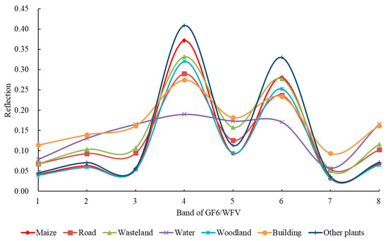
Figure 2.
Spectral curves of different land cover types.
3.2. Class Separability
In this study, JM and TD were used to measure the separability between maize and other land cover types in the research area. The range of JM and TD are within [0, 2]. As a general rule, values in the range of [0.0, 1.0) indicate a very poor class separability; values in the range of [1.0, 1.9) indicate a poor separability; and values in the range of [1.9, 2.0] indicate a relatively good separability.
The class separability of the samples in Table 3 was analyzed, and we found that the separability of different land cover types was significantly different, in whether there was the participation of the new band of GF-6 satellite. Compared with S1, the JM and TD between maize and other plants in S2 increased from 1.32 and 1.43 to 1.80 and 1.97, respectively, and the values between maize and woodland also increased from 1.43 and 1.81 to 1.67 and 1.95, which indicated that B5 can significantly enhance the separability of maize from other plants and wood-lands, but the spectra between them still exhibit a large overlap. By comparing the JM between maize and other land cover types in S1 and S2, we found that B5 also contributes partly to the separability of maize from wasteland and roads. The JM between maize and all land cover types in S3 was unchanged or decreased than that in S2, except between maize and woodland, which indicated that the contribution of B6 to the separability between maize and other land cover types was less than that of B5, but the contribution to the separability between maize and woodland was greater than that of B5. To sum up, the superposition of B5 and B6 can further increase the separability of maize and other land cover types, specifically for the distinction between maize and woodland. In S2, the JM between maize and all other land cover types was greater than 1.8, and the TD was more than 1.9, indicating that when the red-edge wavelength was involved in the calculation, the separability of maize and other land cover types was very high. The purple and yellow bands added in S4 and S5, respectively, can increase the separability of maize and other land cover types in a certain range because they still slightly increase JD, but their effect on improving TD was not obvious.
Table 3.
Separability between maize and other land cover types under different schemes (S1–S5).
3.3. Maize Identification and Classification Results
Using the same training samples, SVM and RF classification models were used to classify the remote sensing image under the S1–S5 schemes. The classification results are shown in Table 4.
Table 4.
Classification results based on support vector machine (SVM) and random forest (RF) models in Qihe County.
The OA of the SVM and RF models under the S1 scheme was quite low at 84.05% and 85.57%, respectively, and the KC was 0.80 and 0.82, respectively. Under the S2 scheme, the classification accuracy of the two classification methods was significantly improved, reaching more than 90%; specifically, the OA of the RF model was 93.24%, and the KC was 0.91. This indicates that Red-edge 1 can effectively improve the classification accuracy of SVM and RF models in the research area. The OA of SVM in the S3 scheme was lower than that in the S2 scheme but remained 5.75% higher than that in the S1 scheme. The total accuracy of RF in the S3 scheme exhibited a significant decline and was far lower than that of the SVM model, but it remained 1.81% higher than that of the S1 scheme. These results indicate that Red-edge 2 can effectively improve the recognition ability of the SVM model on land cover types, but the improvement is lower than that of Red-edge 1. This may be because Red-edge 2 is significantly correlated with NIR (B4; R2 = 0.991; Figure 3a), resulting in feature redundancy. The classification accuracy of the SVM model did not change significantly in the S4 and S5 schemes, and the OA was maintained at approximately 91%, with a KC of 0.89. The OA of the RF model in the S4 scheme increased rapidly compared with the S3 scheme and exceeded the classification result accuracy of the SVM model. The OA was 93.15%, and the KC was 0.91, which was almost the same as the result of the S2 scheme. The OA of the RF model in the S5 scheme was the highest, but it did not change significantly compared with the S4 scheme. The results showed that purple and yellow bands had a limited influence on the classification results. We speculate that one of the reasons may be that B7 was significantly correlated with B1 (R2 = 0.986; Figure 3b), and B8 was significantly correlated with B2 and B3 (R2 = 0.982 and R2 = 0.981; Figure 3c,d).
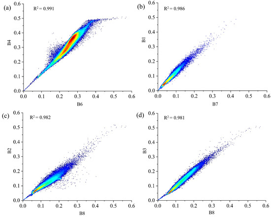
Figure 3.
Correlation analysis between various bands: (a) B4 and B6; (b) B1 and B7; (c) B2 and B8; (d) B3 and B8.
The impact of the newly added bands on the classification results of various land cover types was specifically analyzed, and a confusion matrix was established for the RF model results under the S1–S5 scheme through verification samples (Table 5). Difference analysis results for each land cover type between different band combinations are shown in Table 6.
Table 5.
Confusion matrix for verifying classification accuracy of RF model (unit: %).
Table 6.
Difference analysis results for each land cover type between different band combinations.
The generated confusion matrix indicates that the PA of buildings and water under the S1 scheme was higher, reaching 97.50% and 97.49%, respectively. However, a misclassification between other crops and maize was observed, and the PA of maize is 82.36%. Furthermore, many wastelands and roads were mistakenly divided into buildings. From Figure 4b,h, we intuitively found that there were a large number of road and woodland spots in the RF classification results, as well as a large number of misclassified wastelands.
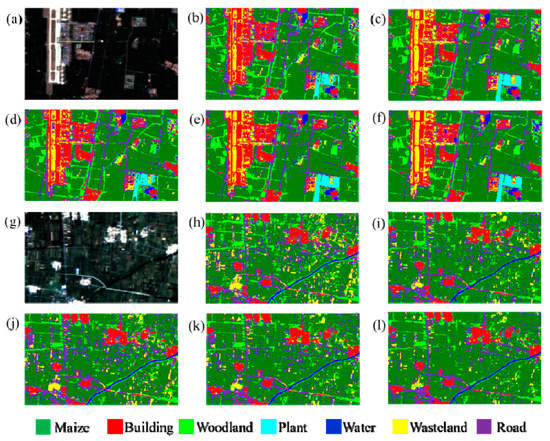
Figure 4.
Classification results of RF models under different band combination schemes: (a) Original image of area A; (b–f) Classification results of S1–S5 in area A; (g) Original image of area B; (h–l) Classification results of S1–S5 in area B.
Under the S2 scheme, with the addition of Red-edge 1, the classification results were significantly improved, especially for woodlands and other plants, and the PA increased from 84.45% and 59.31% to 90.29% and 72.07%, respectively. In particular, the smoothness of the classification results of woodland on both sides of the road was improved (Figure 4c). The classification accuracy of maize reached 97.57%, which was an increase of 15.21% compared to the S1 scheme. However, the classification effect of roads was not significantly improved, and a large number of misclassified discontinuous roads were mixed in the maize fields. It showed that the Red-edge 1 band significantly contributed to vegetation classification, but its role in the recognition of non-vegetation land cover types was limited.
The classification results of S3 with the addition of Red-edge 2 were similar to those of S1 without a significant difference. Although the PA of maize, woodland, and other crops was improved, the PA of water bodies and roads decreased. These results indicated that Red-edge 2 had no obvious effect on improving the classification of land cover types in the research area, particularly for non-vegetation. We intuitively determined that the addition of Red-edge 2 significantly improved the recognition of continuous roads (Figure 4d) and the removal of wasteland patches (Figure 4f). However, the fragmentation of the roads in the field was not reduced. This may be because the resolution of the remote sensing image used was too low to identify a narrow road in the field.
The classification results of the S4 scheme with two red-edge bands were similar to those of the S2 scheme, but the misclassification and omission of almost all vegetation were significantly reduced—specifically, the ability to distinguish maize from other plants was very strong. The classification results exhibited better completeness, and the continuity and smoothness of the boundary of the spots were also improved (Figure 4e). However, Figure 4k shows that discontinuous road spots remained in the classification results. This indicates that when two red-edge bands exist simultaneously, Red-edge 1 plays a major role in classifying land cover types, and Red-edge 2 can be superimposed to improve the classification accuracy of buildings and wasteland.
The S5 scheme with the purple and yellow bands added to the S4 scheme is a remote sensing image that includes all bands of GF-6 WFV and the classification results were not significantly improved. But compared with S4, the PA of roads, wastelands, and water was significantly improved from 83.91%, 68.63%, and 97.46% to 94.89%, 75.97%, and 100%, respectively, indicating that the purple and yellow bands were more likely to respond to non-vegetation and increase their classification accuracy, but the PA of woodland and other vegetation decreased. From the perspective of the entire research area, the purple and yellow bands effectively reduced the “salt-and-pepper phenomenon” in the classification results (Figure 4f,l), thereby improving the accuracy of maize producers to 98.28%.
To sum up, we found that the overall classification accuracy was the best when the RF model was used in the S5 scheme, and the land cover types of Qihe County were extracted as shown in Figure 5. The planting area of maize was estimated with the class statistical tool in ENVI, which was 774.18 km2. According to agricultural statistics, the maize planting area in Qihe County in 2018 was 757.73 km2, which falls within a 2.17% error from our calculated value. As shown in Figure 6, the maize plantation area was the largest, accounting for 54.87% in Qihe County in 2018. These results indicate that maize is a primary food crop in Qihe County; this facilitates a notably high quantity of maize straw being produced in the region, which exhibits great potential for recycling and utilization.
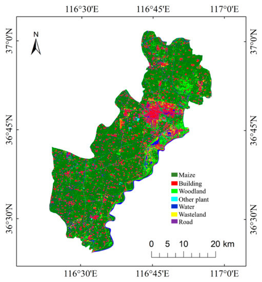
Figure 5.
Land cover types in Qihe County based on the RF model in 2018.
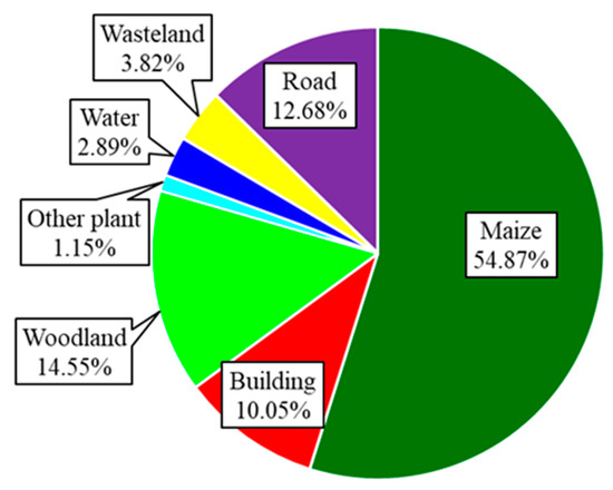
Figure 6.
Land cover type proportions based on the RF model in 2018.
3.4. Spatial Distribution of Maize Straw
Averaging the field survey data in Table 7, the density of maize straw was calculated. According to Equation (1), the spatial distribution of maize straw in 2018 (Figure 7) was obtained by multiplying the planting area (each pixel is 16 m × 16 m) with the density of straw. The distribution of maize straw was the widest in southern and northeastern Qihe County, and the average distribution density in the northernmost and southernmost regions was slightly lower. The central and northern areas exhibit the lowest quantities and average densities because these areas are characterized by numerous towns.
Table 7.
The density of maize straw in the sampling area.
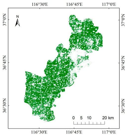
Figure 7.
Spatial distribution of maize straw in Qihe County in 2018.
The total quantity and average density of maize straw in each township were further evaluated, as shown in Figure 8. Although the straw quantities of Liuqiao and An’tou were 47.12 kt and 39.07 kt, respectively, because of the small area of cultivated land, the average maize straw density was 543.46 t/km2 and 525.58 t/km2, respectively, so these two towns were very suitable for maize straw recycling and utilization. Larger townships in the central and southern regions, including Pandian, Renliji, Jiaomiao, and Huguantun, had relatively large maize straw yields and relatively high average density, so the potential for the utilization of maize straw resources was also notable. In northern towns such as Dahuang, Yizhangtun, Biaobaisi, and Huadian and the southern towns such as Zhaoguan and Maji, the total theoretical maize straw quantity was 25–32 kt, with the average density of straw being 380–470 t/km2, which indicates that these towns were also suitable for maize straw recycling and utilization. Yancheng had a small proportion of cultivated land and the lowest average density and yield of maize straw. Due to the development of towns and secondary industries, the average density of maize straw in Zhu’A and Yanbei was also low, indicating that the utilization potential of straw resources is relatively lesser.
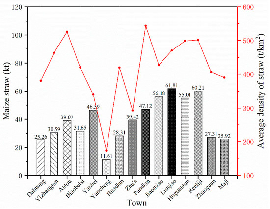
Figure 8.
Statistics of maize straw in each township of Qihe County in 2018.
4. Conclusions
The results of this study show that it is feasible to use SVM and RF models to estimate the yield and spatial distribution of maize straw by combining GF6/WFV, field survey data, and agricultural census. The land cover types in Qihe County were more accurately identified by the RF model, which consequently improved the estimation accuracy of the yield and spatial distribution of the maize straw. The main conclusions are as follows:
- Both SVM and RF models can effectively identify and aid in the classification of land cover types in the research area. The RF model exhibits improved classification accuracy compared to that of SVM when the newly added band of GF-6 WFV was used;
- The addition of two red-edge bands increased the separability of land cover types with large differences in red-side spectral characteristics and generally significantly improved the overall classification accuracy and reduced the misclassification and omission of crops. Red-edge 1 can improve the recognition accuracy of land cover types more than Red-edge 2 in Qihe County. In this study, the classification accuracy and KC of the RF model increased from 85.57% and 0.82 to 93.15% and 0.91, respectively, after adding two red-edge bands;
- The response of purple and yellow bands to non-vegetation was more obvious than that to vegetation, which increased the classification accuracy of non-vegetation and slightly reduced the “salt-and-pepper noise” in the classification results. However, the effects of the two bands on the classification accuracy of vegetation and the total classification accuracy were not obvious;
- The theoretical total quantity of maize straw in Qihe County was 586.08 kt in 2018, which reflected only a 2.42% error from the statistical result. Maize straw in Qihe County was planted, excluding in central and northern urban areas. Among them, the southern and northeastern regions exhibited the widest distribution areas and highest average densities, followed by the northernmost and southernmost regions. The central and northern urban areas exhibited the lowest average distribution densities.
5. Future Work
The research method of this study still exhibits some limitations that should be addressed. After inspection, it was found that the misjudged pixels were primarily those located at the junctions of various land cover types. Many mixed pixels that were difficult to distinguish, even by visual interpretation, were formed in the image because of the superimposed spectral characteristics of different land cover types at the junctions [38]. Concurrently, the spatial resolution of the remote sensing image also limited the accuracy of extraction to a large extent [39]. Therefore, the focus of further research is to fuse higher resolution spatial information, and a discriminant model based on spatial relationship knowledge and mixed pixel decomposition will also be considered to improve extraction accuracy.
Author Contributions
The manuscript was written through the contributions of all authors. Conceptualization, Y.Z. and R.D.; Data curation, H.M.; Formal analysis, H.M. and H.L.; Funding acquisition, Y.Z.; Investigation, H.L.; Methodology, H.M.; Supervision, R.D.; Writing—original draft, H.M.; Writing—review and editing, H.L. and Y.Z. All authors have read and agreed to the published version of the manuscript.
Funding
This study was supported by the National Natural Science Foundation of China (Grant No. U20A2086; 51806242), the Special Project on Innovation Methodology, Ministry of Science and Technology of China (No. 2020IM020900); and the Yantai Educational-Local Synthetic Development Project (Grant No. 2019XDRHXMXK25 and No. 2019XDRHXMQT36).
Institutional Review Board Statement
Not applicable.
Informed Consent Statement
Not applicable.
Data Availability Statement
The data that supported the findings of this study can be available from the corresponding author upon reasonable request.
Acknowledgments
We appreciate the supports from the Key Laboratory of Clean Production and Utilization of Renewable Energy, Ministry of Agriculture and Rural Affairs, at China Agricultural University; the National Joint R&D Center for International Research of BioEnergy Science and Technology, Ministry of Science and Technology, at China Agricultural University; the National Energy R&D Center for Biomass, National Energy Administration of China, at China Agricultural University; and Beijing Municipal Key Discipline of Biomass Engineering.
Conflicts of Interest
The authors declare no competing financial and non-financial interests.
References
- Jiao, X.; Mongol, N.; Zhang, F. The transformation of agriculture in China: Looking back and looking forward. J. Integr. Agric. 2018, 17, 755–764. [Google Scholar] [CrossRef]
- El-Dewany, C.; Awad, F.; Zaghloul, A.M. Utilization of rice straw as a low-cost natural by-product in agriculture. Int. J. Environ. Pollut. Environ. Model. 2018, 1, 91–102. [Google Scholar]
- Nie, P.; Sousa-Poza, A.; Xue, J. Fuel for life: Domestic cooking fuels and women’s health in rural China. Int. J. Environ. Res. Public Health 2016, 13, 810. [Google Scholar] [CrossRef]
- Cui, M.; Zhao, L.; Tian, Y.; Meng, H.; Sun, L.; Zhang, Y.; Wang, F.; Li, B. Analysis and evaluation on energy utilization of main crop straw resources in China. Trans. Chin. Soc. Agric. Eng. 2008, 24, 291–296. (In Chinese) [Google Scholar]
- Wang, Y.; Bi, Y.; Gao, C. The assessment and utilization of straw resources in China. Agric. Sci. China 2010, 9, 1807–1815. [Google Scholar] [CrossRef]
- Ren, J.; Yu, P.; Xu, X. Straw utilization in China—Status and recommendations. Sustainability 2019, 11, 1762. [Google Scholar] [CrossRef]
- Hong, J.; Ren, L.; Hong, J.; Xu, C. Environmental impact assessment of corn straw utilization in China. J. Clean. Prod. 2016, 112, 1700–1708. [Google Scholar] [CrossRef]
- Wang, B.; Shen, X.; Chen, S.; Bai, Y.; Yang, G.; Zhu, J.; Shu, J.; Xue, Z. Distribution characteristics, resource utilization and popularizing demonstration of crop straw in southwest China: A comprehensive evaluation. Ecol. Indic. 2018, 93, 998–1004. [Google Scholar] [CrossRef]
- Abdel-Mohdy, F.A.; Abdel-Halim, E.S.; Abu-Ayana, Y.M.; El-Sawy, S.M. Rice straw as a new resource for some beneficial uses. Carbohyd. Polym. 2009, 75, 44–51. [Google Scholar] [CrossRef]
- Venturini, G.; Pizarro-Alonso, A.; Münster, M. How to maximise the value of residual biomass resources: The case of straw in Denmark. Appl. Energy 2019, 250, 369–388. [Google Scholar] [CrossRef]
- Bi, Y.Y.; Wang, Y.J.; Gao, C.Y. Straw Resource quantity and its regional distribution in China. J. Agric. Mech. Res. 2010, 3, 1–7. [Google Scholar]
- Long, H.; Li, X.; Wang, H.; Jia, J. Biomass resources and their bioenergy potential estimation: A review. Renew. Sust. Energy Rev. 2013, 26, 344–352. [Google Scholar] [CrossRef]
- Moxey, A.; Mcclean, C.J.; Allanson, P. Transforming the spatial basis of agricultural census cover data. Soil Use Manag. 2010, 11, 21–25. [Google Scholar] [CrossRef]
- Galanopoulos, C.; Odierna, A.; Barletta, D.; Zondervan, E. Design of a wheat straw supply chain network in Lower Saxony, Germany through optimization. Comput. Aided Chem. Eng. 2017, 40, 871–876. [Google Scholar]
- Zhou, L.; Gu, W.; Zhang, Q. Logistics mode and network planning for recycle of crop straw resources. Asian Agric. Res. 2013, 5, 87. [Google Scholar]
- Ballesteros, R.; Ortega, J.F.; Hernandez, D.; Del Campo, A.; Moreno, M.A. Combined use of agro-climatic and very high-resolution remote sensing information for crop monitoring. Int. J. Appl. Earth Obs. Geoinf. 2018, 72, 66–75. [Google Scholar] [CrossRef]
- Kern, A.; Barcza, Z.; Marjanović, H.; Árendás, T.; Fodor, N.; Bónis, P.; Bognár, P.; Lichtenberger, J. Statistical modelling of crop yield in Central Europe using climate data and remote sensing vegetation indices. Agric. For. Meteorol. 2018, 260, 300–320. [Google Scholar] [CrossRef]
- Atzberger, C. Advances in remote sensing of agriculture: Context description, existing operational monitoring systems and major information needs. Remote Sens. 2013, 5, 949–981. [Google Scholar] [CrossRef]
- Duveiller, G.; Defourny, P. A conceptual framework to define the spatial resolution requirements for agricultural monitoring using remote sensing. Remote Sens. Environ. 2010, 114, 2637–2650. [Google Scholar] [CrossRef]
- Vrieling, A.; Skidmore, A.K.; Wang, T.; Meroni, M.; Ens, B.J.; Oosterbeek, K.; O’Connor, B.; Darvishzadeh, R.; Heurich, M.; Shepherd, A. Spatially detailed retrievals of spring phenology from single-season high-resolution image time series. Int. J. Appl. Earth Obs. Geoinf. 2017, 59, 19–30. [Google Scholar] [CrossRef]
- Wang, L.; Liu, J.; Yang, F.; Yao, B.; Shao, J.; Yang, L. Rice recognition ability basing on GF-1 multi-temporal phases combined with near infrared data. Trans. Chin. Soc. Agric. Eng. 2017, 33, 196–202. (In Chinese) [Google Scholar]
- Li, S.; Zhao, J.; Dong, S.; Zhao, M.; Li, C.; Cui, Y.; Liu, Y.; Gao, J.; Xue, J.; Wang, L. Advances and prospects of maize cultivation in China. Sci. Agric. Sin. 2017, 50, 1941–1959. [Google Scholar]
- Xu, W. A LM-2D Launches GF-6 Satellite. Aerosp. China 2019, 19, 60. [Google Scholar]
- Tong, X.; Zhao, W.; Xing, J.; Fu, W. In Status and development of china high-resolution earth observation system and application. In Proceedings of the 2016 IEEE International Geoscience and Remote Sensing Symposium (IGARSS), Beijing, China, 10–15 July 2016; pp. 3738–3741. [Google Scholar]
- Young, N.E.; Anderson, R.S.; Chignell, S.M.; Vorster, A.G.; Lawrence, R.; Evangelista, P.H. A survival guide to Landsat preprocessing. Ecology 2017, 98, 920–932. [Google Scholar] [CrossRef]
- Lantzanakis, G.; Mitraka, Z.; Chrysoulakis, N. Comparison of physically and image based atmospheric correction methods for Sentinel-2 satellite imagery. In Perspectives on Atmospheric Sciences; Bais, A., Nastos, P., Eds.; Springer International Publishing: Cham, Switzerland, 2017; pp. 255–261. [Google Scholar]
- Mountrakis, G.; Im, J.; Ogole, C. Support vector machines in remote sensing: A review. ISPRS J. Photogramm. Remote Sens. 2011, 66, 247–259. [Google Scholar] [CrossRef]
- Breiman, L. Random forests. Mach. Learn. 2001, 45, 5–32. [Google Scholar] [CrossRef]
- Thanh Noi, P.; Kappas, M. Comparison of random forest, k-nearest neighbor, and support vector machine classifiers for land cover classification using Sentinel-2 imagery. Sensors 2018, 18, 18. [Google Scholar] [CrossRef]
- Du, P.; Xia, J.; Chanussot, J.; He, X. Hyperspectral remote sensing image classification based on the integration of support vector machine and random forest. In Proceedings of the 2012 IEEE International Geoscience and Remote Sensing Symposium, Munich, Germany, 22–27 July 2012; pp. 174–177. [Google Scholar]
- Van der Linden, S.; Rabe, A.; Held, M.; Jakimow, B.; Leitão, P.J.; Okujeni, A.; Schwieder, M.; Suess, S.; Hostert, P. The EnMAP-Box—A Toolbox and Application Programming Interface for EnMAP Data Processing. Remote Sens. 2015, 7, 11249–11266. [Google Scholar] [CrossRef]
- Gambarova, Y.M.; Gambarov, A.Y.; Rustamov, R.B.; Zeynalova, M.H. Remote sensing and GIS as an advance space technologies for rare vegetation monitoring in Gobustan State National Park, Azerbaijan. J. Geogr. Inf. Syst. 2010, 2, 93. [Google Scholar] [CrossRef]
- Weiser, C.; Zeller, V.; Reinicke, F.; Wagner, B.; Majer, S.; Vetter, A.; Thraen, D. Integrated assessment of sustainable cereal straw potential and different straw-based energy applications in Germany. Appl. Energy 2014, 114, 749–762. [Google Scholar] [CrossRef]
- Tharwat, A. Classification assessment methods. Appl. Comput. Inform. 2020, 17, 168–192. [Google Scholar] [CrossRef]
- Ai, B.; Sheng, Z.; Zheng, L.; Shang, W. Collectable amounts of straw resources and their distribution in China. In Advances in Engineering Research, Proceedings of the International Conference on Advances in Energy, Environment and Chemical Engineering, Changsha, China, 26–27 September 2015; Atlantis Press: Paris, France, 2015; pp. 441–444. [Google Scholar]
- Jawak, S.D.; Luis, A.J. Improved land cover mapping using high resolution multiangle 8-band WorldView-2 satellite remote sensing data. J. Appl. Remote Sens. 2013, 7, 73573. [Google Scholar] [CrossRef]
- Martinez, L.J.; Ramos, A. Estimation of chlorophyll concentration in maize using spectral reflectance. Int. Arch. Photogramm. Remote Sens. Spat. Inf. Sci. 2015, 40, 65. [Google Scholar] [CrossRef]
- Löw, F.; Duveiller, G. Defining the spatial resolution requirements for crop identification using optical remote sensing. Remote Sens. 2014, 6, 9034–9063. [Google Scholar] [CrossRef]
- Kempeneers, P.; Sedano, F.; Seebach, L.; Strobl, P.; San-Miguel-Ayanz, J. Data fusion of different spatial resolution remote sensing images applied to forest-type mapping. IEEE Trans. Geosci. Remote Sens. 2011, 49, 4977–4986. [Google Scholar] [CrossRef]


Publisher’s Note: MDPI stays neutral with regard to jurisdictional claims in published maps and institutional affiliations. |
© 2021 by the authors. Licensee MDPI, Basel, Switzerland. This article is an open access article distributed under the terms and conditions of the Creative Commons Attribution (CC BY) license (https://creativecommons.org/licenses/by/4.0/).