The Heterogeneous Public Debt–Growth Relationship: The Role of the Expenditure Multiplier

Abstract

Currently countries are facing a new crisis caused by the COVID-19, which leads to the rise of government expenditures and additional borrowing. This situation highlights the importance of examine factors which determine the level of public debt that still sustains economic growth. A growing body of research supports the idea of a non-linear debt–growth relationship and estimates the threshold level above which debt becomes unsustainable and has a negative effect on output. The empirical evidence points out that there is no single sustainable debt threshold level that holds for all countries. This research complements scarce empirical evidence on the heterogeneous debt–growth relationship and provides some insights on the publicly available statistical indicators that might signal a relatively low/high expenditure multiplier and, at the same time, potentially unsustainable/sustainable growth stimulus through the use of borrowed funds. We test the hypothesis that the expenditure multiplier is shaping the impact of public debt on growth. Our empirical examination is based on panel data analysis in the groups of countries with expected relatively high and low expenditure multiplier. Research results show that a statistically significant negative marginal effect of debt on growth starts to manifest at a lower debt-to-GDP ratio when the expenditure multiplier is lower and vice-versa. The study shed some light on the sources of heterogeneity in a debt–growth relationship. We can conclude that countries with a high expenditure multiplier level can borrow more and sustain growth. In contrast, in countries with a lower expenditure multiplier, a relatively low debt level becomes unsustainable for growth.

1. Introduction

The economic crisis in 2008–2009 has led to an unprecedented increase in public debt. However, recovery has remained sluggish, raising serious concerns about the impact of public debt on economic growth. In their seminal paper, Reinhart and Rogoff [1] argued that public debt to GDP ratio higher than 90% is harmful to economic growth. Their study inspired research on the debt threshold level in various countries and regions, and many studies found the support for the idea of non-linear debt–growth relationship and the existence of the threshold level above which debt becomes unsustainable and restricts output growth. However, the results of the research are contradictory in assessing the level of debt from which its impact on growth changes from positive to negative (see [2,3] for systematic review).

Nowadays, countries are facing a new crisis caused by the coronavirus (COVID-19), which leads to further rise in public borrowing. At the same time, debt levels remain high in many countries after dealing with the economic crisis in 2008–2009. The new borrowing of the countries should be consistent with fiscal spending and deficit plans; the government’s borrowing decisions should be carefully set to keep public debt on a sustainable path. This situation highlights the importance to examine what factors determine the level of public debt that still sustains growth? However, to our best knowledge, there is relatively scarce empirical evidence on this question. Review of research [4] suggests that institutions shape the debt–growth nexus and debt threshold is higher for countries with better institutions. The state of the financial market [5], country risk [6], economic systems [7], trade balance [8] are confirmed as well as the factors shaping the impact of debt on growth.

The positive effect of debt is grounded on the Keynesian view that expansionary fiscal policy leads to a higher debt level, but it simultaneously stimulates the private demand and output growth through the mechanism of the fiscal multiplier. The question of how government debt affects the size of the fiscal multiplier raises debate in the literature. Nonetheless, empirical results suggest an inverse relationship between these two variables [9,10,11,12,13,14,15,16,17]. The lower the expenditure multiplier, the weaker the positive impact of government spending and thus of public debt on the economy, and debt is less sustainable. Our research complements scarce empirical evidence on the heterogeneous debt–growth relationship by raising the assumption that the expenditure multiplier is shaping the impact of public debt on growth and we put forward a hypothesis that countries with a higher expenditure multiplier have a higher debt threshold level.

Immense empirical studies have examined the impact of public debt on output; however, Huidrom et al. [18] point to the lack of systematic investigation on the channels through which public debt affects the fiscal multiplier. Contributing to a limited literature on this issue, this paper provides the theoretical background for how a fiscal multiplier may decline in response to growing public debt and in turn potentially lower the impact of public debt on economic growth. The fiscal multiplier determines the effectiveness of the fiscal policy but paradoxically gives no practical insights to its application, as there is no consensus in the literature on both the size of fiscal multiplier and the method of measuring it [11]. In response to this, our research aims to provide some insights on the publicly available statistical indicators that might signal a relatively low/high fiscal multiplier and, at the same time, potentially unsustainable/sustainable growth stimulus through the use of borrowed funds.

The empirical examination is based on the analysis of panel data and results indicate the positive debt threshold dependence on the expenditure multiplier, but irrespective of its size only low levels of public debt have positive and statistically significant links with economic growth. At the same time, the levels of public debt that hinder economic growth clearly depend on the indicators that reflect the size of the expenditure multiplier.

The rest of the paper is organised as follows: Section 2 discusses channels through which public debt can potentially have an impact on sustainable economic growth and the fiscal multiplier; it presents a review of empirical evidence on the relationship between public debt and the fiscal multiplier. Section 3 presents the methodology of the research, i.e., the model, data and estimation strategy. Section 4 presents and discusses the estimation results. The last section concludes the paper.

2. Literature Review

2.1. Public Debt’s Impact on Economic Growth and Fiscal Multiplier

There are diverse channels through which public debt can potentially have an impact on economic growth. In the literature the positive effect of public debt on growth is grounded on the Keynesian view that expansionary fiscal policy leads to higher debt level but simultaneously stimulates domestic demand and thus GDP growth through the mechanism of the fiscal multiplier. The positive effect of government spending depends on the size of the expenditure multiplier, which is positively related to marginal propensities to consume and invest and is negatively related to the tax rate and marginal propensity to import. The debt level has no direct positive effect on economic growth and can be hardly distinguished from the government spending effect. Following that, the expenditure multiplier determines the impact of both government expenditure and public debt on economic growth and can serve as a factor explaining estimated varying public debt–growth relationships across countries.

Huidrom et al. [18] point to vast empirical evidence that weak public finances impede the effectiveness of the fiscal policy. However, the channels through which public debt can have an impact on fiscal multipliers have not yet been systematically investigated. Growing debt can have an adverse effect on private consumption and investment decisions and, at the same time, on the expenditure multiplier simultaneously depressing the effectiveness of the fiscal policy. This negative impact is more likely to occur or to be more pronounced at higher debt levels, explaining the non-linear debt–growth relationship.

The negative impact of public debt on private investment, consumption, and economic growth originates from various channels. The crowding-out effect on investments and consumption occurs due to a rise in interest rates. Increased government borrowing leads to higher GDP, higher demand for money and hence to higher interest rates, considering that the money supply is constant. Rising interest rates may reduce the private investment (and marginal propensity to invest) and increase households’ incentives to save and reduce consumption (decrease in marginal propensity to consume) [17]. However, this negative effect may not occur at the zero-lower bound (ZLB). Horvath et al. [19] following the New Keynesian model suggest that increase in government spending is followed by growing output and inflation, which decreases the real interest rate, as the nominal interest rate is fixed at ZLB. Declining real interest rate stimulates consumption, investment, and output, therefore avoiding the crowding-out effect. Priftis and Zimic [20] find that a way of financing government spending determines whether the crowding-out or crowding-in effect on private investment may be expected. If spending is financed abroad, investment is crowded in, while home-debt financed spending produces a crowding out of private investment.

The established link between public debt and interest rates does not necessarily support the presence of the crowding-out effect through increased demand for money channels. The increase in interest rates may originate from the risk premium channel. Usually, countries with high debt levels pay a risk premium [21,22]. Results of many empirical studies [22,23,24,25] confirm that, above a certain threshold of debt, the (market) interest rate on public debt increases with the debt level (as a percentage of GDP).

The twin deficit hypothesis explains the crowding-out effect of budget deficit (growing public debt) on net exports. Budget deficit refers to increased public spending, which in turn stimulates domestic income. Countries with a higher marginal propensity to import will tend to import more as domestic incomes rise, what will lead to a higher trade deficit and slower economic growth. According to the literature, the level of trade openness reduces the magnitude of the expenditure multiplier [15]. In addition, Butkus and Seputiene [8] estimated a lower debt threshold level for countries with a higher level of trade deficit.

The growth reducing effects of public debt arise due to the increase in uncertainty about fiscal policy in the future. The Ricardian equivalence hypothesis emphasises that rising debt requires higher government revenues for debt repayment. This raises uncertainty about taxes in the future and can potentially impact incentives to save and invest. Preparing for higher taxation in future, households save more and reduce consumption (the marginal propensity to consume declines). If private consumers perceive the current debt level as unsustainable, they may increase precautionary saving to a large degree [13]. However, the review of the research on validity of Ricardian equivalence theorem points to generally inconclusive findings [26].

According to Munir and Mehmood [27], a high public debt level may serve as a signal of higher uncertainty about countries’ economic conditions and discourage investments. Huidrom et al. [18] confirm a negative public debt effect on the government spending multiplier to operate through private consumption and sovereign risk premium channels. The impulse responses of private consumption to government spending are conditional on public debt level. Positive government spending shock decreases private consumption and raises CDS spreads (risk premium variable) when the debt level is high. In times of strong fiscal position, private consumption reacts to fiscal stimulus in a Keynesian manner, while CDS spreads do not respond significantly and remain broadly constant. Anzuini et al. [28] present discussion of the effects arising from fiscal policy uncertainty and estimate different outcomes of the same change in the government budget, depending on whether fiscal policy uncertainty is increasing or decreasing. Keynesian effects of expansionary fiscal policy prevail only if policy implementation decreases (or at least does not increase) uncertainty. Empirical estimations confirm the negative effect of rising government spending uncertainty [29] and changes in uncertainty about fiscal policy [30] on private consumption and investment.

Growing debt increases uncertainty, but effects may vary across countries with different qualities of institutions [4]. Caner et al. [31] conclude that advanced economies have a higher debt threshold level than developing ones. This can be related to better institutional quality, higher trust in public institutions and thus lower uncertainty in developed countries. The empirical evidence on the role of institutions in shaping the growth effect of public debt is relatively scarce, but mostly confirms that better institutional quality allows borrowing more without harming the economy (for a detailed review, see [4]).

In summary, the positive impact of debt on economic growth depends on the size of the expenditure multiplier, but rising debt can reduce it through the impact on consumption, investment, and trade deficit.

2.2. Empirical Evidence on the Relationship between Public Debt and the Fiscal Multiplier

The studies present inconsistent results on the question of how government debt affects the size of the fiscal multiplier. Kirchner et al. [9] conclude that increasing government debt in the euro area leads to a smaller expenditure multiplier after five years. Silva et al. [12] present a similar conclusion and estimate that tax and spending cumulative 10-year-period multipliers for the euro area decrease once the dynamic of public debt is controlled. Afonso and Leal [15] in a sample of 19 Eurozone countries estimated a higher expenditure multiplier for countries with a lower public debt-to-GDP ratio, with a dividing threshold of 60%. Using a neoclassical model calibrated to Greece, Wang [17] confirms that public consumption and public investment multipliers depend on a country’s debt level. Expansionary effects of public spending differ in a high-debt and a low-debt economy and are determined by implementation delays, the degree of public and private consumption complementarity, and the speed of tax adjustments.

Auerbach and Gorodnichenko [10] find that a large debt reduces the government spending multiplier in OECD countries. Ilzetzki et al. [11] find a lower expenditure multiplier in high debt countries and estimate a 60 percent debt threshold above which government consumption has a negative effect on output. Nickel and Tudyka [13] in a sample of 17 European countries confirm expansionary effects of public spending on the macroeconomic activity at low debt levels, but the overall positive effect on real GDP decreases or even becomes negative at higher debt-to-GDP ratios. Kim’s [14] findings suggest that the multiplier in a high-debt US states is larger than in a low-debt states. Atems [16] comes to a similar conclusion when using panel structural VAR analyses and finds a larger government spending multiplier for US states during episodes of low debt compared to periods of high debt.

Contrary to these findings, other studies suggest the public debt having no significant effect on the fiscal multiplier. Corsetti et al. [32] focus on 17 OECD countries and estimate the impact response of output, investment, consumption, net exports, real exchange rate, inflation, and real interest rate to government spending shocks. They made the distinction between countries with sound and weak public finances (the gross government debt-to-GDP ratio is, respectively lower or higher than 100%) and find only moderate differences in estimated responses. IMF [33] estimations for advanced economies do not confirm that the public investment multiplier depends on the initial public-debt-to-GDP ratio. However, such results can be related to the lower debt share in GDP in advanced economies. Bi et al. [34] present simulation results that government spending in low-debt US states is more expansionary than in high-debt states. However, this conclusion is not robust to alternative specifications. Adi [35] analyses how public and private debt levels shape the effect of spending and revenue stimulus on GDP growth in a balanced panel of 16 countries and an unbalanced panel of 39 countries. The results do not provide any robust evidence that public debt has an influence on how government expenditure or revenue affects GDP growth. Boitani and Perdichizzi [36] in a panel of 12 euro area countries find a similar output response to government spending in the countries with high and low public debt.

A possible explanation for the abovementioned inconsistency of the results is that the impact of public debt on fiscal multiplier is time-varying and non-linear, occurring only at a certain debt level. Aloui and Eyquem [37] present simulation results showing that the initial debt level lowers the public spending multiplier in normal times but increases it at the ZLB. This can be explained by the fact that spending is self-financing at the ZLB, as output increases, pushing the debt-to-GDP ratio down, then allowing a decrease in tax rates. The higher initial debt level is, the larger the decline in taxes is, leading to a more significant boost in output.

If we agree that the positive effect of public debt on economic growth is related to the expenditure multiplier and that increasing debt reduces its size, this may explain why the debt–economic growth relationship is non-linear and we expect countries with a low expenditure multiplier to have a lower debt threshold, when the growth-enhancing effect changes to a growth-inhibiting one. However, to our knowledge, there is little if no discussion in the literature on the role of factors the fiscal multiplier depends on in explaining the heterogeneity of public debt impact on economic growth.

3. Methods and Data

To examine the non-linear debt–growth relationship, we rely on Cobb–Douglas trans-log specification of the neo-classical growth Equation:

$$\frac{1}{T}ln\left(\frac{Y_{i, t+T}}{Y_{i,t}}\right)={\beta }_0+{\beta }_{1}ln\left(Y_{i,t}\right)+{\beta }_{2}ln\left(D_{i,t}\right)+{\beta }_3{\left[ln\left(D_{i,t}\right)\right]}^2+{\beta }_{3+k}{\mathit{C}}_{k,i,t}+{\theta }_t+{\mu }_i+{\epsilon }_{i,t},$$

(1)

where $\frac{1}{T}ln\left(\frac{Y_{i, t+T}}{Y_{i,t}}\right)$ stands for the average yearly growth rate in country i over the period from t to T. $Y_{i,t}$ is the per capita GDP at constant prices, $D_{i,t}$—debt, and ${\mathit{C}}_{k,i,t}$ is the vector of growth controls. ${\theta }_t$ and ${\mu }_i$ are time-varying and country-specific effects, respectively, modelled including time dummies and estimating Equation (1) using LSDV. ${\epsilon }_{i,t}$ is the idiosyncratic error term. ${\beta }_{(·)}$ are parameters to be estimated. The estimated positive coefficient on ${\beta }_2$ and negative on ${\beta }_3$ would give empirical evidence of a debt–growth nexus in the form of an inverted U-shaped letter. The threshold debt level is equal to $e^{-\frac{\widehat{{\beta }_2}}{2\widehat{{\beta }_3}}}$. The marginal effect of debt on growth is calculated as ${\beta }_2+2{\beta }_{3}ln\left(D_{i,t}\right)$. Since the marginal effect depends on the value of $ln\left(D_{i,t}\right)$, it is conditional. Since not just the marginal effect is conditional but the standard error associated with it is conditional too, the standard errors are calculated, using formulas provided by Dawson (2014). This specification allows us to estimate which level of debt is sustainable, i.e., positively affects economic growth and the tipping point above which debt does not sustain growth. It also allows visualisation of whether the marginal effect of debt on growth is significant at different levels of indebtedness.

Estimating Equation (1), we have to select the span of the growth episode (T) facing several trade-offs related to this selection. T = 1 (i.e., using annual per capita GDP growth) allows maximisation of the sample size. Still, this strategy might lead to estimates that are highly affected by the cyclical patterns of economic fluctuations and endogeneity (since debt is lagged only by one period with respect to growth). These issues are usually addressed by setting T equal to 5 and aiming to estimate the effect of the current level of debt (and the other left-hand-side variables) on the 5-year forward non-overlapping average per capita GDP growth rate. Aiming to mitigate the endogeneity bias in Equation (1), it is common in the empirical growth literature to use forward-looking averages. Since current growth rates (or the expected growth rate over the next year) affect debt, just like debt affects growth rates, averaged future values can, to some degree, prevent a reverse causality. Nevertheless, this strategy significantly reduces the sample size and introduces some uncertainty considering the first and last usable observations. As an alternative, we consider using 5-year overlapping growth periods. However, the usage of overlapping growth rates as the dependent variable creates a moving average structure in the error term. Following Panizza and Presbitero [38], we use the Huber–White Sandwich correction, which yields almost identical results as Newey and West’s [39] estimator, which allows modelling of the autocorrelation in the error term.

Our empirical analysis is based on an unbalanced panel of 138 countries from 1996 to 2016 (see Appendix A). Our sample includes countries from different geographical regions representing different stages of development and covers the whole period (and all countries) for which the necessary statistical data were available. It allows us to increase the variation of public debt as well as other variables that may affect the debt–growth nexus. Following the survey on public debt and the economic growth relationship [3,40], the period is divided into one-, five- and ten-year overlapping intervals to study a short-, middle-, and long-run relationship between debt and growth.

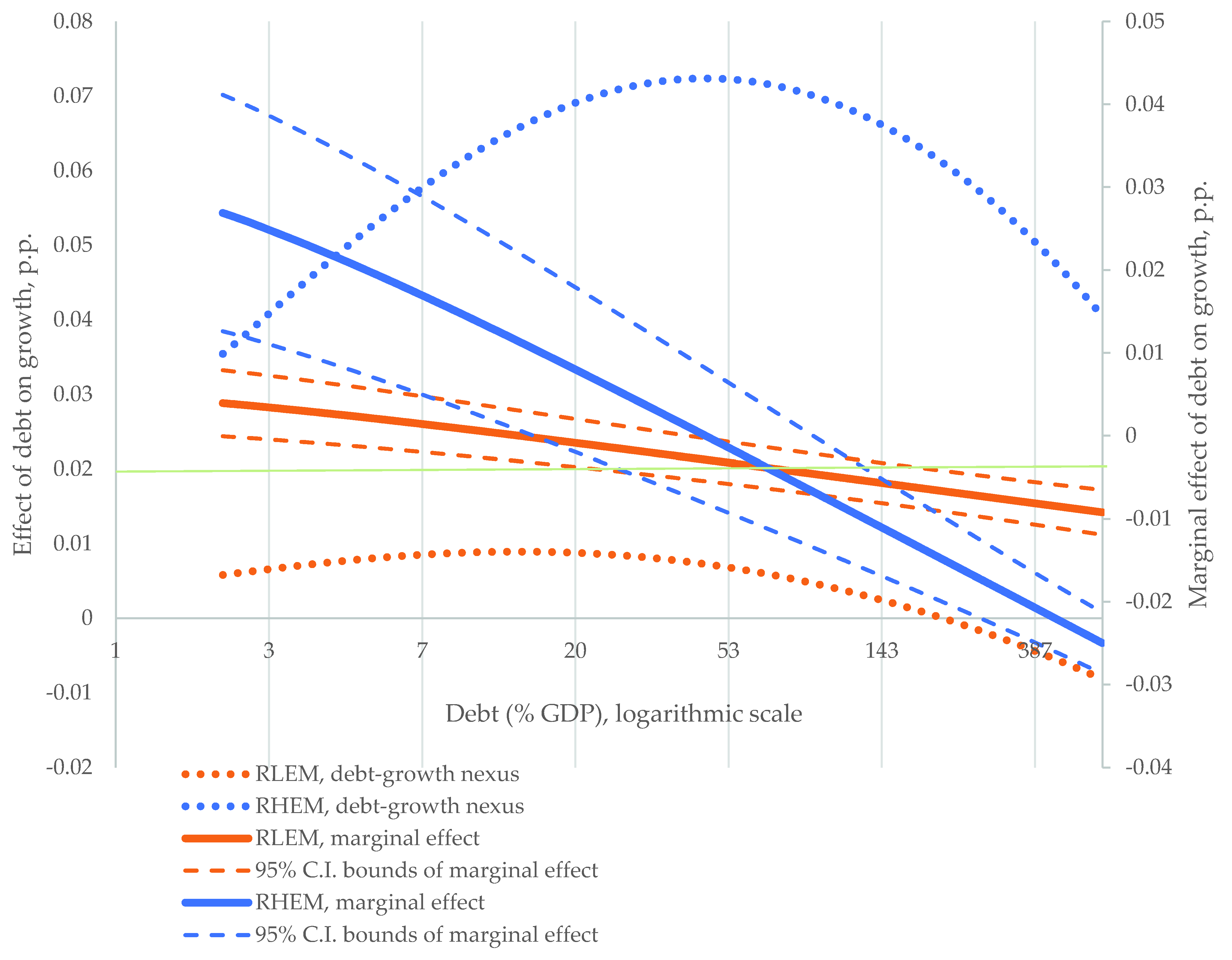
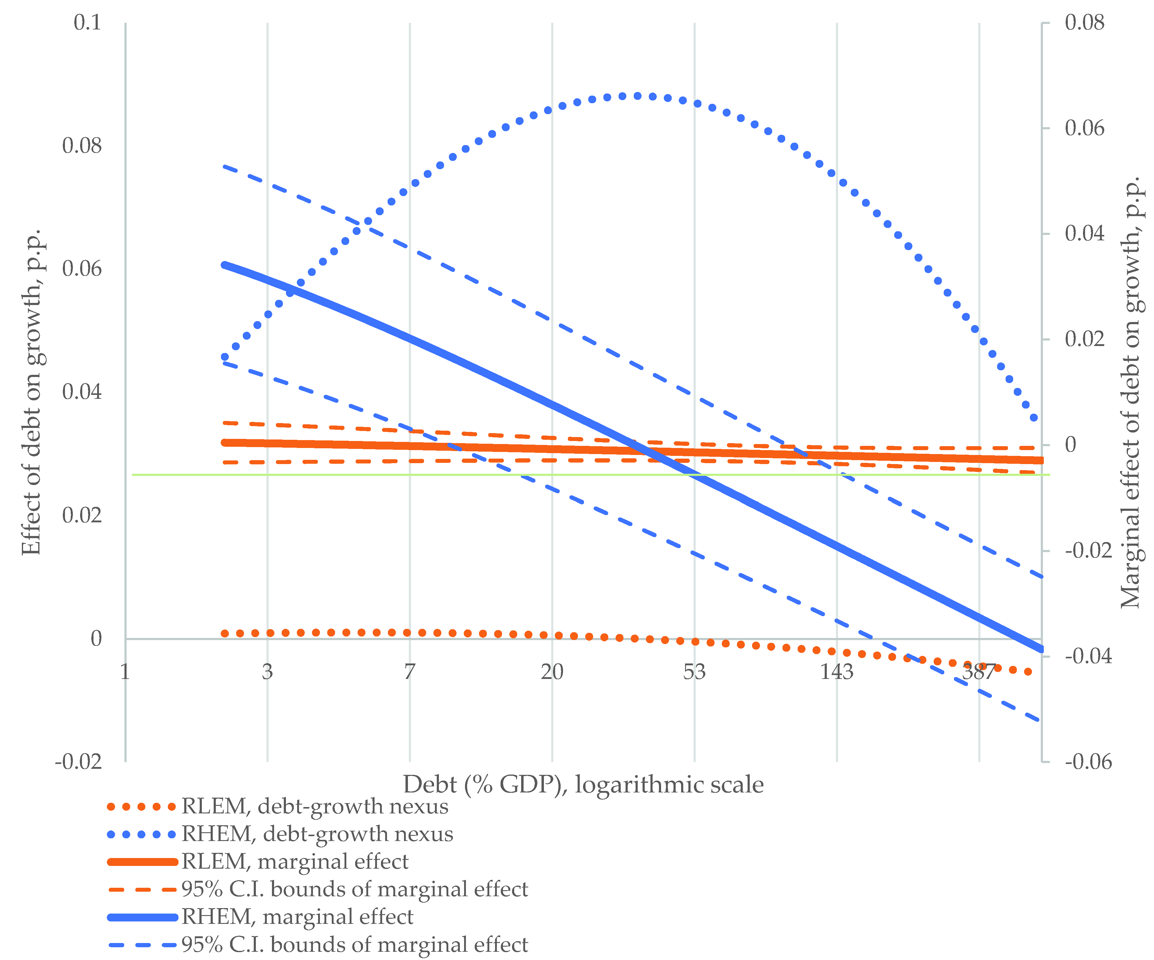
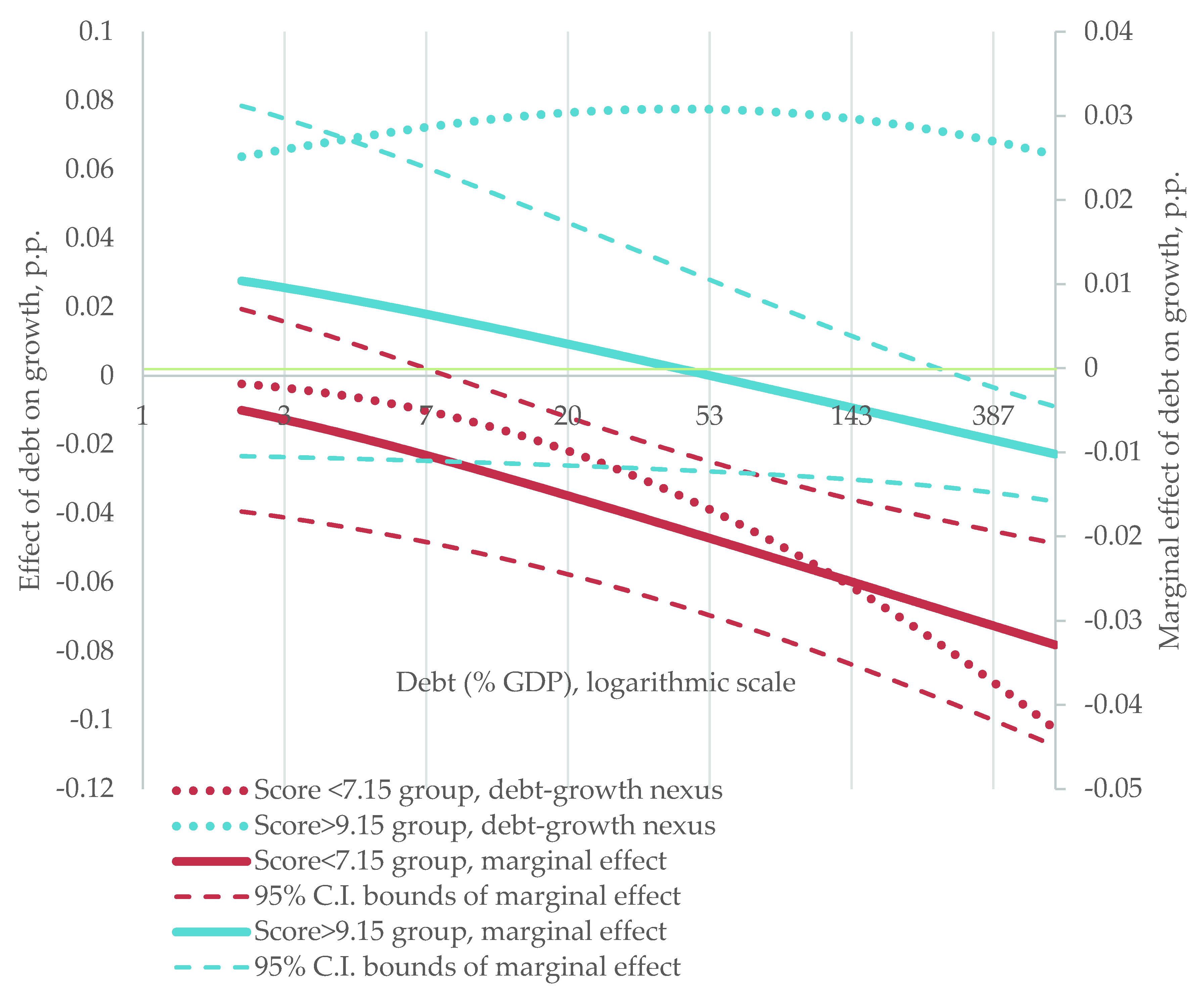
Our research tests an assumption that the impact of public debt on economic growth depends on the size of the expenditure multiplier. However, the magnitude of the multiplier at a given moment is indefinite, and there is no consensus on its estimation [11]. Our research applied a methodology similar to Batini et al. [41], and the expected size of the expenditure multiplier was estimated following two steps. First, we assigned scores to the country based on how many characteristics are associated with a “large” multiplier. Second, summing the scores, we determined the likely level of the multiplier. Therefore, in this study, we split countries into two sub-samples according to whether economic indicators signal the higher or lower expected value of the multiplier.

Berti et al. [42] focus on the impact that different assumptions about fiscal multipliers have on the projected dynamics of the public debt ratio. To group low or high multiplier level countries, they chose indicators of long-term sovereign bond spread, financial institutions’ credit growth, the unemployment rate, considering that these indicators are expected to have an impact on consumption and investment decisions and in that way reflect the expected size of the fiscal multiplier. In our study, we choose indicators that directly reflect consumption and investment volumes. Since the expenditure multiplier positively depends on the marginal propensity to consume, the marginal propensity to invest, and negatively on the tax rate and the marginal propensity to import, to approximate these variables, we used the share of consumption, the share of investment, the share of taxes, and the share of imports in GDP, respectively. Hubbard [43] acknowledged that, over the long-run, the differences between marginal and average propensities tend to decrease. Here, we do not claim that the certain values of these indicators correspond to a high or low multiplier; the distribution is conditional, based on the cross-country comparison.

In the spirit of [20,44], we condition sample splitting on descriptive statistics of country characteristics. We assigned scores from 1 to 3 to each value of the indicator. The score reflects the potential indicator’s effect on the size of the multiplier in a way that a higher score is assigned if the multiplier is expected to be higher. The range of observed indicator’s values was divided into three intervals in such a way that one-third of all observations would fall in one of the intervals. The upper and lower thresholds for the indicator’s values are as follows:

• For the share of consumption in GDP: <58.2%—Score 1 is assigned; from 58.2% up to 71.5%—Score 2; >71.5%—Score 3.
• For the share of investment in GDP: <19.5%—Score 1 is assigned; from 19.5% up to 25.3%—Score 2; >25.3%—Score 3.
• For the share of taxes in GDP: <13.4%—Score 3 is assigned; from 13.4% up to 19.8%—Score 2; >19.8%—Score 1.
• For the share of imports in GDP: <27%—Score 3 is assigned; from 27% up to 46% of GDP—Score 2; >46%—Score 1.

The total score, ranging from 4 up to 12, was calculated by summing up scores of separate indicators. Scores were estimated only if data were available on all four indicators. The total score was firstly calculated for each year and then averaged (min. 4.83, max. 11.56). According to the ranking used in this study, a higher total score indicates a higher value of the multiplier. The country is considered as a having relatively low expenditure multiplier (subsample RLEM) if the score is below the median level, i.e., 8.15 (see

Table A1. List of countries with a relatively low expenditure multiplier.

Angola	Czech Republic	Lithuania	Slovakia
United Arab Emirates	Denmark	Luxembourg	Slovenia
Australia	Estonia	Latvia	Sweden
Austria	Finland	Morocco	Seychelles
Belgium	France	Malta	Togo
Bulgaria	United Kingdom	Mongolia	Tajikistan
Bahrain	Croatia	Mozambique	Tunisia
Bosnia and Herzegovina	Hungary	Mauritius	Ukraine
Belarus	Ireland	Malaysia	South Africa
Belize	Iceland	Namibia	Zimbabwe
Barbados	Israel	Netherlands	Marshall Islands
Bhutan	Italy	Norway	Palau
Botswana	Jamaica	New Zealand	Papua New Guinea
Canada	Jordan	Poland	Timor-Leste
Côte d’Ivoire	Kuwait	Portugal	Vanuatu
Congo	Liberia	Singapore
Cabo Verde	Saint Lucia	El Salvador
Cyprus	Lesotho	Serbia

Notes: A country is considered as having a relatively low expenditure multiplier if the score is below the median level (8.15). In the Italics, we distinguish countries with scores below 7.15. The total number of countries with a relatively low multiplier is 69, with a score below 7.15–36.

in Appendix A). Otherwise, a country is considered as having relatively high expenditure multiplier (subsample RHEM, see

Table A2. List of countries with a relatively high expenditure multiplier.

Albania	Germany	Japan	Philippines
Argentina	Dominican Republic	Kazakhstan	Paraguay
Armenia	Egypt	Kenya	Romania
Azerbaijan	Spain	Kyrgyzstan	Russian Federation
Burundi	Ethiopia	Cambodia	Rwanda
Benin	Gabon	Republic of Korea	Saudi Arabia
Burkina Faso	Georgia	Lebanon	Sudan
Bangladesh	Ghana	Sri Lanka	Senegal
Bahamas	Guinea	Republic of Moldova	Thailand
Bolivia (Plurinational State of)	Gambia	Madagascar	Turkey
Brazil	Guinea-Bissau	Mexico	Uganda
Central African Republic	Greece	North Macedonia	Uruguay
Switzerland	Guatemala	Mali	United States
Chile	Honduras	Myanmar	Uzbekistan
China	Indonesia	Niger	Zambia
Cameroon	India	Nicaragua
Colombia	Iran (Islamic Republic of)	Nepal
Costa Rica	Iraq	Peru

Notes: A country is considered as having a relatively high expenditure multiplier if the score is above the median level (8.15). In the Italics, we distinguish countries with scores above 9.15. The total number of countries with a relatively low multiplier is 69, with a score above 9.15–30.

in Appendix A).

Table 1. Variables for estimating score on expenditure multiplier.

Variable	Subsample	Mean	S.D.	Min	Max
Imports (% GDP) (1)	RLEM	52.0	28.40	0.007	236.0
	RHEM	29.1	15.30	0.016	109.0
Gross capital formation (% GDP) (1)	RLEM	21.7	8.38	0.008	95.3
	RHEM	24.3	7.95	0.021	70.2
Tax revenue (% GDP) (1)	RLEM	20.7	7.11	0.044	62.9
	RHEM	12.4	3.98	0.890	26.3
Household consumption (% GDP) (1)	RLEM	60.1	16.40	10.900	166.0
	RHEM	69.9	14.80	12.070	228.0

Note: ⁽¹⁾ The World Bank’s World Development Indicator’s database.

shows the descriptive statistics of variables used to determine the size of the multiplier.

Table 2. Variables, source of data and descriptive statistics.

Variable	Subsample	Mean	S.D.	Min	Max
Annual growth rate, %	RLEM	2.22	5.03	−37.60	65.30
	RHEM	1.89	6.48	−65.01	87.70
Five-year average growth rate, %	RLEM	2.23	3.48	−24.00	33.00
	RHEM	1.94	4.17	−34.00	42.80
Ten-year average growth rate, %	RLEM	1.98	2.33	−13.80	15.90
	RHEM	1.76	2.95	−15.80	27.90
Y, GDP per capita (constant 2010 USD) (1)	RLEM	16,441	18,956	164	116,230
	RHEM	6264	11,040	132	77,684
D, General government gross debt (% GDP) (2)	RLEM	56.40	42.30	0.03	515.00
	RHEM	57.00	46.40	0.07	495.00
G, Government size, General government final consumption expenditure (% of GDP) (1)	RLEM	18.90	7.16	2.05	136.00
	RHEM	13.20	5.04	0.09	46.00
HC, Human capital, School enrolment, secondary (% gross) (1)	RLEM	77.80	32.50	2.34	164.00
	RHEM	54.40	32.80	1.01	129.00
ACPI, Inflation, Average consumer prices index, (2) (% change)	RLEM	16.10	142.00	−72.70	4734.90
	RHEM	40.50	377.00	−31.30	11,961.00
GE, Government effectiveness (estimate) (3)	RLEM	−0.311	0.782	−2.23	2.18
	RHEM	0.469	1.020	−1.88	2.44
POP, Population growth. Total population, (1) (% change)	RLEM	1.55	1.81	−3.77	19.30
	RHEM	1.97	1.25	−6.54	9.19
T, Trade (Exports plus imports as a % of GDP) (1)	RLEM	99.20	55.50	23.20	437.00
	RHEM	53.00	27.40	0.02	167.00
GCF, Investments, Gross capital formation (% of GDP) (1)	RLEM	21.7	8.38	0.056	95.3
	RHEM	24.3	7.95	0.013	70.2

⁽¹⁾ The World Bank’s World Development Indicator’s database. ⁽²⁾ The International Monetary Fund’s World Economic Outlook’s database. ⁽³⁾ The World Bank’s World Governance Indicator’s database.

presents all variables used in the regression analysis.

4. Results and Discussion

4.1. General Results

Table 3. LSDV estimates of debt—five-year average growth rate nexus.

Variable	Parameter	Relatively Low Expenditure Multiplier	Relatively High Expenditure Multiplier
Intercept	β0	0.2929 *	0.7944 ***
		(0.1580)	(0.0918)
Initial per capita GDP, ln(Y)	β1	−0.0598 ***	−0.1208 ***
		(0.0126)	(0.0072)
Debt, ln(D)	β2	0.0067	0.0376 ***
		(0.0059)	(0.0086)
Squared debt, [ln(D)]2	β3	−0.0012	−0.0049 ***
		(0.0010)	(0.0012)
Government effectiveness, GE (1)	β4	0.0016	0.0020
		(0.0074)	(0.0034)
Human capital, ln(HC)	β5	0.0003	0.0309 ***
		(0.0081)	(0.0056)
Trade, ln(T)	β6	0.0291 ***	0.0101 **
		(0.0078)	(0.0044)
Inflation, Δln(ACPI)	β7	−0.0564 **	−0.0231 *
		(0.0268)	(0.0124)
Population growth, Δln(POP)	β8	−0.7418 **	−0.7364 ***
		(0.3508)	(0.0963)
Government size, ln(G)	β9	−0.0294 ***	−0.0172 ***
		(0.0087)	(0.0051)
Investments, ln(GCF)	β10	0.1269 **	0.1082 ***
		(0.0554)	(0.0338)
Squared investments, [ln(GCF)]2	β11	−0.0207 **	−0.01713 ***
		(0.0091)	(0.0053)
Estimated debt threshold level, %		14	47
Number of observations		627	694
Number of countries		63	69
Average observations per group		9.95	10.06
LSDV R2		0.7506	0.7769
Within R2		0.3554	0.6434
Pesaran CD test for cross-sectional dependence (2) [p-value]		[0.659]	[0.482]
Test for differing group intercepts (3) [p-value]		[<0.001]	[<0.001]
Wald joint test on time dummies (4) [p-value]		[<0.001]	[<0.001]
Hausman test (5) [p-value]		[<0.001]	[<0.001]

Notes: ⁽¹⁾ Government effectiveness is the only variable that takes negative values and enters the model in not logged form. ⁽²⁾ A low p-value counts against the null hypothesis: cross-sectional independence. ⁽³⁾ A low p-value counts against the null hypothesis: the groups have a common intercept. ⁽⁴⁾ A low p-value counts against the null hypothesis: no time effects. ⁽⁵⁾ A low p-value counts against the GLS estimates with random effects in favour of LSDV. Heteroscedasticity robust standard errors are presented in parentheses. All estimations include time and country effects, and Huber–White Sandwich correction. *, **, *** indicate significance at the 10, 5 and 1 percent levels, respectively.

presents estimates of Equation (1) for the five-year average growth rate. Appendix B and Appendix C present estimates for the annual growth rate and ten-year average growth rate, respectively.

The estimates on control variables are mainly consistent with findings in previous research [4,7,8,44,45,46,47,48] and in line with economic theory. Estimates show that countries are converging since 1 percent higher per capita GDP is associated with 0.06–0.12 percentage points slower growth and vice versa. Government effectiveness, human capital and trade positively correlate with economic growth, whereas government size, inflation and population growth constrain growth. Capital investments have a diminishing marginal effect on growth. Similar relationships show estimates with annual growth rate and ten-year average growth rate which are presented in Appendix B and Appendix C. However, as regards control variables, some differences can also be observed compared to the results of other researchers. The negative effect of trade openness is observed in countries with weak institutions [8,44,45]; other studies find a positive impact of population growth [7,8,48].

Like in most empirical research on non-linear debt–growth relationships (see review of results in references [3,4]) our estimates provide evidence that this link is in the form of an inverted U-shaped letter. Megersa and Cassimon [46] highlight that countries with better quality of governance and institutional environment have a higher public debt sustainability threshold and empirical evidence supports this conclusion [4]. However, few studies [49,50,51] find opposite results, i.e., that the negative effect of debt on growth increases as institutional quality improves. Our estimates suggest that the size of the expenditure multiplier may be another potential source of a heterogenous debt–growth relationship. The threshold level is at about 14% of debt-to-GDP ratio for the countries with relatively low expenditure multipliers, whereas the turning point is higher at about 47% for the countries with a relatively high multiplier. The same tendency, i.e., higher turning point in a sample of countries with higher expenditure multiplier, holds for estimates with annual growth rate and ten-year average growth rate presented in Appendix B and Appendix C. Estimates show that the negative marginal effect of debt on growth starts to manifest, having a lower debt-to-GDP ratio when the expenditure multiplier is lower and vice versa. As the group of countries with a relatively low (high) multiplier includes countries with high (low) government efficiency, our results to some extent support findings [8] that good governance is not enough to a avoid negative public debt effect on growth.

Figure 1 presents the effect of debt on the five-year growth rate for both groups of countries.

We can see that sign, size, as well as the statistical significance of the marginal effect, vary depending on the debt size. A positive and statistically significant (when the 95% C.I. does not contain zero) marginal effect of debt on growth occurs when the debt level is below 2% and 16% for relatively low and relatively high multiplier countries, respectively. The marginal effect of debt on growth is negative and statistically significant (when the 95% C.I. does not contain zero) when the debt level exceeds 42% and 92% for relatively low and relatively high multiplier countries, respectively. The marginal effect is statistically insignificant if debt-to-GDP is between 3% and 42% and between 17% and 92% for relatively low and relatively high multiplier countries, respectively. Since the curve which represents the debt–growth nexus for relatively high multiplier countries is above one for relatively low multiplier countries, to some extent, our estimates support the assumption that positive debt impact on growth is more pronounced if macroeconomic indicators are favourable for higher expenditure multiplier effect to occur. It follows that the debt turning point is higher in countries with a relatively higher expenditure multiplier.

Figures on the debt-growth nexus for annual growth rate and ten-year average growth rate are presented in Appendix B and Appendix C.

Table 4. Non-linear debt–growth nexus.

Effect on	Subsample	The Size of Debt (% GDP) When the Estimated Marginal Effect of Debt on Growth Is:
		Positive and Statistically Significant	Statistically Insignificant	Negative and Statistically Significant
The five-year average growth rate	RLEM	1–2	3–42	>42
	RHEM	1–16	17–92	>92
Annual growth rate	RLEM	-	1–64	>64
	RHEM	1–16	17–104	>104
The ten-year average growth rate	RLEM	-	1–17	>17
	RHEM	-	1–138	>138

summarises our findings and shows that much higher indebtedness is needed in the countries with the relatively higher expenditure multiplier for a debt to have a negative and statistically significant effect on growth.

The estimated debt turning points should be considered with caution. Eberhardt and Presbitero [52], Gómez-Puig and Sosvilla-Rivero [48,53], Ahlborn and Schweickert [7] suggest that it is worthless to look for a debt threshold that holds for all countries (or country groups). Eberhardt and Presbitero [52] indicate that a country’s ability to increase the debt level without facing a slowdown effect on the economy may depend the on various country-specific factors. Studies confirm great variability of the debt threshold level across countries [2,3], but most of them do not provide an explanation for such heterogeneity [7]. The estimated debt threshold levels in Table 4 shed some light on the sources of heterogeneity in debt–growth relationship. They support the assumption that the sustainable growth effect of public debt may vary with the size of expenditure multiplier and suggest a detrimental effect to occur at a higher debt to GDP ratios if macroeconomic indicators (consumption, investments, taxes, and import shares in GDP) are more favourable to a higher value of the expenditure multiplier in a country.

As the size of the expenditure multiplier is indefinite at any given time, when considering whether the level of public debt is on a sustainable path, fiscal policymakers should pay attention to available macroeconomic indicators, which may in part provide information on the potential magnitude of the multiplier effect. However, in order to provide a practical guidance to policy makers, more detailed studies are needed.

4.2. Robustness Check

For a robustness check, we estimated our model for the subsamples of the countries with relatively more extreme scores for the expenditure multiplier (removing from the sample the countries with “typical scores”, i.e., medial level ±1), assuming that we would find more distinct values of indebtedness that lead to a negative debt–growth nexus that would strengthen our general findings. Estimation results are presented in Appendix D (see

Table A5. LSDV estimates of the debt–growth nexus.

Variable	Parameter	Annual Growth Rate		Five-Year Average Growth Rate		Ten-Year Average Growth Rate
		Score < 7.15	Score > 9.15	Score < 7.15	Score > 9.15	Score < 7.15	Score > 9.15
Intercept	β0	−0.0331	1.2440 ***	0.4188 **	0.6845 **	0.5115 ***	0.6028 ***
		(0.3795)	(0.1771)	(0.1705)	(0.3148)	(0.0964)	(0.1039)
Initial per capita GDP, ln(Y)	β1	−0.0504 **	−0.1454 ***	−0.0464 ***	−0.1555 ***	−0.0511 ***	−0.0769 ***
		(0.0238)	(0.0103)	(0.0108)	(0.0191)	(0.0071)	(0.0059)
Debt, ln(D)	β2	0.0008	0.0147	0.0066 **	0.0393 ***	0.0041 ***	0.0068
		(0.0073)	(0.0125)	(0.0027)	(0.0103)	(0.0011)	(0.0090)
Squared debt, [ln(D)]2	β3	−0.0026 *	−0.0019	−0.0025 ***	−0.0049 ***	−0.0008 ***	−0.0008
		(0.0015)	(0.0018)	(0.0006)	(0.0015)	(0.0003)	(0.0012)
Government effectiveness, GE (1)	β4	0.0002	0.0030	0.0009 ***	0.0037	0.0009 **	0.0030
		(0.0046)	(0.0154)	(0.0003)	(0.0074)	(0.0004)	(0.0040)
Human capital, ln(HC)	β5	0.0067 *	0.0158 **	0.0309 **	0.0081 ***	0.0070	0.0056 ***
		(0.0035)	(0.0064)	(0.0154)	(0.0029)	(0.0046)	(0.0016)
Trade, ln(T)	β6	0.0186 ***	0.0383 ***	0.0506 ***	0.0201 ***	0.0087 **	0.0017
		(0.0065)	(0.0130)	(0.0120)	(0.0060)	(0.0034)	(0.0038)
Inflation, Δln(ACPI)	β7	−0.0594 ***	−0.0231	−0.1456 ***	−0.0257	−0.0058	−0.0158
		(0.0182)	(0.0487)	(0.0396)	(0.0197)	(0.0108)	(0.0098)
Population growth, Δln(POP)	β8	−0.6978 ***	−0.0728	−0.8968 ***	0.1066	−0.0401	−0.1612
		(0.1605)	(0.6735)	(0.3223)	(0.2667)	(0.1056)	(0.1436)
Government size, ln(G)	β9	−0.0392 ***	−0.0275 *	−0.0441 ***	−0.0021	−0.0093 ***	−0.0012
		(0.0072)	(0.0148)	(0.0138)	(0.0072)	(0.0035)	(0.0039)
Investments, ln(GCF)	β10	0.1374 *	0.2467	0.3403 **	0.1084	0.1059 **	0.0861 **
		(0.0730)	(0.1503)	(0.1419)	(0.0661)	(0.0409)	(0.0366)
Squared investments, [ln(GCF)]2	β11	−0.0237 **	−0.0375	−0.0484 **	−0.0182 *	−0.0190 ***	−0.0143 **
		(0.0115)	(0.0240)	(0.0224)	(0.0106)	(0.0064)	(0.0060)
Estimated debt threshold level, %		1.16	47.87	3.64	54.94	11.33	70
Number of observations		538	351	416	264	296	173
Number of countries		36	30	34	30	34	26
Average observations per group		14.94	11.7	12.24	8.80	8.71	6.65
LSDV R2		0.5780	0.4469	0.7897	0.8503	0.9083	0.9494
Within R2		0.5209	0.2042	0.7219	0.4095	0.8142	0.4929
Pesaran CD test for cross-sectional dependence (2) [p-value]		[0.156]	[0.441]	[0.232]	[0.187]	[0.254]	[0.148]
Test for differing group intercepts (3) [p-value]		[<0.001]	[<0.001]	[<0.001]	[<0.001]	[<0.001]	[<0.001]
Wald joint test on time dummies (4) [p-value]		[<0.001]	[<0.001]	[<0.001]	[<0.001]	[<0.001]	[<0.001]
Hausman test (5) [p-value]		[<0.001]	[<0.001]	[<0.001]	[<0.001]	[<0.001]	[<0.001]

Notes: ⁽¹⁾ Government effectiveness is the only variable that takes negative values and enters the model in not logged form. ⁽²⁾ A low p-value counts against the null hypothesis: cross-sectional independence. ⁽³⁾ A low p-value counts against the null hypothesis: the groups have a common intercept. ⁽⁴⁾ A low p-value counts against the null hypothesis: no time effects. ⁽⁵⁾ A low p-value counts against the GLS estimates with random effects in favour of LSDV. Heteroscedasticity robust standard errors are presented in parentheses. All estimations include time and country effects, and Huber–White Sandwich correction. *, **, *** indicate significance at the 10, 5 and 1 percent levels, respectively.

), and

Table 5. Summary results of the robustness check.

Effect on	Multiplier Score	The Size of Debt (% GDP) When the Estimated Marginal Effect of Debt on Growth Is:
		Positive and Statistically Significant	Statistically Insignificant	Negative and Statistically Significant
The five-year average growth rate	Score < 7.15	1	2–7	>7
	Score > 9.15	1–13	14–154	>154
Annual growth rate	Score < 7.15	-	1	>1
	Score > 9.15	-	1–264	>264
The ten-year average growth rate	Score < 7.15	1–3	4–32	>32
	Score > 9.15	-	>0	-

summarises the findings.

The results show that a smaller debt-to-GDP ratio is needed for the countries with a relatively very low expenditure multiplier (scores < 7.15) to reach the point when debt starts to constrain growth compared to findings in Table 4 where the countries with scores < 8.15 are included. Similarly, a higher debt-to-GDP ratio is needed for the countries with a relatively very high expenditure multiplier (score > 9.15) to reach the point when debt starts to constrain growth compared to findings in Table 4 where the countries with scores > 8.15 are included.

5. Conclusions

The economic theory explains the growth stimulative effect of public debt through the impact of expansionary fiscal policy, the effectiveness of which is directly related to the size of the fiscal multiplier. It follows that the multiplier shapes the impact of both public expenditure and debt on growth. The empirical studies mostly concentrate on the relationship between debt level and the size of the fiscal multiplier, while the strand of empirical research on heterogeneous debt impact on output, as far as we know, mostly ignores the determinants of the fiscal multiplier as possible explanatory variables determining the debt tipping point, above which a growth-suppressive effect occurs. The overwhelming empirical evidence confirms that this negative impact becomes more pronounced at higher debt levels, with no consensus on what debt to GDP ratio becomes harmful to economy or what factors drive that ratio.

There are relatively few studies evaluating the factors that determine why in some countries the negative impact on economic growth is manifested as a lower debt ratio while in others as a higher debt-to-GDP ratio. It is generally confirmed that the institutional environment determines the marginal impact of debt on economic growth and the size of the debt threshold. Studies on other potential factors of the heterogeneous impact of debt on economic growth are very limited. Contributing to this limited literature, our research tests the hypothesis that the expenditure multiplier is shaping the impact of public debt on growth. As the growth effect of public debt depends on the size of the expenditure multiplier, this paper raises the assumption that indicators shaping the size of the expenditure multiplier (marginal propensities to consume and invest, marginal propensity to import, and tax rate) can serve as factors, explaining what debt to GDP ratios become harmful to economic growth.

Estimates confirm the research hypothesis and show that a negative marginal effect of debt on growth starts to manifest, showing a lower debt-to-GDP ratio when the multiplier is lower and vice-versa. We do not find robust evidence that public debt has a positive effect on growth since the debt to GDP interval with a statistically significant and positive effect on growth is very narrow with respect to the expenditure multiplier. As in other studies (see a review of results in references [3,4]), our empirical estimations provide evidence that the non-linear debt–growth relationship is in the form of an inverted U-shaped letter. Our estimates suggest that the size of the expenditure multiplier may be another potential source of heterogeneous debt-to-growth ratios relationship.

The estimated debt threshold levels shed some light on the sources of heterogeneity in a debt–growth relationship. They support the assumption that the sustainable growth effect of public debt may vary with the size of the expenditure multiplier and suggest detrimental effects to occur at a higher debt to GDP ratios if macroeconomic indicators (consumption, investments, taxes, and import shares in GDP) are more favorable to a higher value of the expenditure multiplier in a country. These statements allow us to conclude that the same level of debt can be sustainable and unsustainable. It depends on the size of the expenditure multiplier: countries with a relatively high expenditure multiplier can borrow more and debt remains sustainable for growth; in countries with a relatively low multiplier, even a small debt ratio can become unsustainable.

As the size of the expenditure multiplier is indefinite at any given time, fiscal policymakers, when considering whether the level of public debt is on a sustainable path, should pay attention to available macroeconomic indicators, which may in part provide information on the potential magnitude of the multiplier effect. However, in order to provide practical guidance to policy makers, more detailed further research is needed, namely: (a) whether all of the indicators analysed are equally important in respect to the heterogeneity of debt effects since the assumption that all are equally important could be seen as the limitation of our study, (b) to examine whether there is threshold level of consumption, investment, taxes or imports (as share in GDP) above/below which negative debt impact on growth is more likely to occur.

The main limitation of our specification in the research is an assumption that just an expenditure multiplier is affecting the debt–growth nexus. Further research could develop a specification that would allow us to examine the interaction between the institutional framework and expenditure multiplier as a source of the heterogeneous debt–growth relationship.

References

1. Reinhart, C.M.; Rogoff, K.S. Growth in a time of debt. Am. Econ. Rev. 2010, 100, 573–578. [Google Scholar] [CrossRef] [Green Version]
2. Rahman, N.H.A.; Ismail, S.; Ridzuan, A.R.; McMillan, D. How does public debt affect economic growth? A systematic review. Cogent Bus. Manag. 2019, 6, 1–21. [Google Scholar] [CrossRef]
3. Bentour, E.M. On the public debt and growth threshold: One size does not necessarily fit all. Appl. Econ. 2021, 53, 1280–1299. [Google Scholar] [CrossRef]
4. Law, S.H.; Ng, C.H.; Kutan, A. Public debt and economic growth in developing countries: Nonlinearity and threshold analysis. Econ. Model. 2021, 98, 26–40. [Google Scholar] [CrossRef]
5. Proaño, C.R.; Schoder, C.; Semmler, W. Financial stress, sovereign debt and economic activity in industrialised countries: Evidence from dynamic threshold regressions. J. Int. Money Financ. 2014, 45, 17–37. [Google Scholar] [CrossRef] [Green Version]
6. Chiu, Y.; Lee, C. On the impact of public debt on economic growth: Does country risk matter? Contemp. Econ. Policy 2017, 35, 751–766. [Google Scholar] [CrossRef]
7. Ahlborn, M.; Schweickert, R. Public debt and economic growth—Economic systems matter. Int. Econ. Econ. Policy 2018, 15, 373–403. [Google Scholar] [CrossRef] [Green Version]
8. Butkus, M.; Seputiene, J. Growth effect of public debt: The role of government effectiveness and trade balance. Economies 2018, 6, 62. [Google Scholar] [CrossRef] [Green Version]
9. Kirchner, M.; Cimadomo, J.; Hauptmeier, S. Transmission of Government Spending Shocks in the Euro Area: Time Variation and Driving Forces; European Central Bank: Frankfurt am Main, Germany, 2010. [Google Scholar]
10. Auerbach, A.J.; Gorodnichenko, Y. Fiscal multipliers in recession and expansion. In Fiscal Policy after the Financial Crisis; Alesina, A., Giavazzi, F., Eds.; University of Chicago Press: Chicago, IL, USA, 2013; pp. 63–98. [Google Scholar]
11. Ilzetzki, E.; Mendoza, E.G.; Végh, C.A. How big (small?) are fiscal multipliers? J. Monet. Econ. 2013, 60, 239–254. [Google Scholar] [CrossRef] [Green Version]
12. Silva, R.; Carvalho, V.M.; Ribeiro, A.P. How Large Are Fiscal Multipliers? A Panel-Data Var Approach for the Euro Area; University of Porto: Porto, Portugal, 2013. [Google Scholar]
13. Nickel, C.; Tudyka, A. Fiscal stimulus in times of high debt: Reconsidering multipliers and twin deficits. J. Money Credit Bank. 2014, 46, 1313–1344. [Google Scholar] [CrossRef] [Green Version]
14. Kim, W. Do government spending multipliers depend on the level of government debt? US historical data evidence. Appl. Econ. Lett. 2015, 22, 668–672. [Google Scholar] [CrossRef]
15. Afonso, A.; Leal, F.S. Fiscal multipliers in the Eurozone: An SVAR analysis. Appl. Econ. 2019, 51, 5577–5593. [Google Scholar] [CrossRef]
16. Atems, B. The effects of government spending shocks: Evidence from U.S. states. Reg. Sci. Urban Econ. 2019, 74, 65–80. [Google Scholar] [CrossRef]
17. Wang, S.L. Fiscal stimulus in a high-debt economy? A DSGE analysis. Econ. Model. 2021, 98, 118–135. [Google Scholar] [CrossRef]
18. Huidrom, R.; Kose, M.A.; Lim, J.J.; Ohnsorge, F.L. Why do fiscal multipliers depend on fiscal positions? J. Monet. Econ. 2020, 114, 109–125. [Google Scholar] [CrossRef] [Green Version]
19. Horvath, R.; Kaszab, L.; Marsal, A.; Rabitsch, K. Determinants of fiscal multipliers revisited. J. Macroecon. 2020, 63, 103162. [Google Scholar] [CrossRef]
20. Priftis, R.; Zimic, S. Sources of borrowing and fiscal multipliers. Econ. J. 2021, 131, 498–519. [Google Scholar] [CrossRef]
21. Alcidi, C.; Gros, D. Public Debt and the Risk Premium: A Dangerous Doom Loop; CEPS: Brussels, Belgium, 2019. [Google Scholar]
22. Blanchard, O. Public debt and low interest rates. Am. Econ. Rev. 2019, 109, 1197–1229. [Google Scholar] [CrossRef] [Green Version]
23. Engen, E.M.; Hubbard, R.G. Federal Government Debt and Interest Rates; National Bureau of Economic Research: Cambridge, MA, USA, 2004. [Google Scholar] [CrossRef]
24. Ardagna, S.; Caselli, F.; Lane, T. Fiscal discipline and the cost of public debt service: Some estimates for OECD countries. BE J. Macroecon. 2007, 7, 1–35. [Google Scholar] [CrossRef] [Green Version]
25. Laubach, T. New evidence on the interest rate effects of budget deficits and debt. J. Eur. Econ. Assoc. 2009, 7, 858–885. [Google Scholar] [CrossRef] [Green Version]
26. Hayo, B.; Neumeier, F. The (in)validity of the Ricardian equivalence theorem–findings from a representative German population survey. J. Macroecon. 2017, 51, 162–174. [Google Scholar] [CrossRef] [Green Version]
27. Munir, K.; Mehmood, N.R. Exploring the channels and impact of debt on economic growth: Evidence from South Asia. South Asia Econ. J. 2018, 19, 171–191. [Google Scholar] [CrossRef]
28. Anzuini, A.; Rossi, L.; Tommasino, P. Fiscal policy uncertainty and the business cycle: Time series evidence from Italy. J. Macroecon. 2020, 65, 103–238. [Google Scholar] [CrossRef]
29. Kim, W. Government spending policy uncertainty and economic activity: US time series evidence. J. Macroecon. 2019, 61, 103124. [Google Scholar] [CrossRef]
30. Fernández-Villaverde, J.; Guerrón-Quintana, P.; Kuester, K.; Rubio-Ramírez, J. Fiscal volatility shocks and economic activity. Am. Econ. Rev. 2015, 105, 3352–3384. [Google Scholar] [CrossRef] [Green Version]
31. Caner, M.; Grennes, T.; Koehler-Geib, F. Finding the Tipping Point—When Sovereign Debt Turns Bad; World Bank: Washington, DC, USA, 2010. [Google Scholar] [CrossRef]
32. Corsetti, G.; Meier, A.; Müller, G.J. What determines government spending multipliers? Econ. Policy 2012, 27, 521–565. [Google Scholar] [CrossRef] [Green Version]
33. IMF. Chapter 3. Is it time for an infrastructure push? The macroeconomic effects of public investment. In World Economic Outlook, October 2014: Legacies, Clouds, Uncertainties; International Monetary Fund: Washington, DC, USA, 2014; pp. 75–112. [Google Scholar] [CrossRef]
34. Bi, H.; Shen, W.; Yang, S.-C.S. Debt-dependent effects of fiscal expansions. Eur. Econ. Rev. 2016, 88, 142–157. [Google Scholar] [CrossRef] [Green Version]
35. Adi, C. Do public and private debt levels affect the size of fiscal multipliers? J. Indones. Econ. Bus. 2017, 32, 209–233. [Google Scholar] [CrossRef] [Green Version]
36. Boitani, A.; Perdichizzi, S. Public Expenditure Multipliers in Recessions: Evidence from the Eurozone; Università Cattolica del Sacro Cuore, Dipartimento di Economia e Finanza (DISCE): Milano, Italy, 2018. [Google Scholar]
37. Aloui, R.; Eyquem, A. Spending multipliers with distortionary taxes: Does the level of public debt matter? J. Macroecon. 2019, 60, 275–293. [Google Scholar] [CrossRef] [Green Version]
38. Panizza, U.; Presbitero, A.F. Public debt and economic growth: Is there a causal effect? J. Macroecon. 2014, 41, 21–41. [Google Scholar] [CrossRef] [Green Version]
39. Newey, W.K.; West, K.D. Hypothesis testing with efficient method of moments estimation. Int. Econ. Rev. 1987, 28, 777–787. [Google Scholar] [CrossRef]
40. Panizza, U.; Presbitero, A.F. Public debt and economic growth in advanced economies: A survey. Swiss. J. Econ. Stat. 2013, 149, 175–204. [Google Scholar] [CrossRef] [Green Version]
41. Batini, N.; Eyraud, L.; Forni, L.; Weber, A. Fiscal Multipliers: Size, Determinants, and Use in Macroeconomic Projections; International Monetary Fund: Washington, DC, USA, 2014. [Google Scholar] [CrossRef]
42. Berti, K.; De Castro, F.; Salto, M. Effects of Fiscal Consolidation Envisaged in the 2013 Stability and Convergence Programmes on Public Debt Dynamics in EU Member States; European Commission Directorate-General for Economic and Financial Affairs Publications: Brussels, Belgium, 2013. [Google Scholar]
43. Hubbard, J. The marginal and average propensities to consume. Q. J. Econ. 1954, 68, 83–96. [Google Scholar] [CrossRef]
44. Turan, T.; Yanıkkaya, H. External debt, growth and investment for developing countries: Some evidence for the debt overhang hypothesis. Port. Econ. J. 2020. [Google Scholar] [CrossRef]
45. Cordella, T.; Ricci, L.A.; Ruiz-Arranz, M. Debt overhang or debt irrelevance? IMF Staff Pap. 2010, 57, 1–24. [Google Scholar] [CrossRef]
46. Megersa, K.; Cassimon, D. Public debt, economic growth, and public sector management in developing countries: Is there a link? Public Admin. Dev. 2015, 35, 329–346. [Google Scholar] [CrossRef] [Green Version]
47. Sigue, M.; Coulibaly, M. Evaluation of the non-linear effects of the public debt on the economic growth of the WAEMU. Res. Econ. Manag. 2020, 5, 63–80. [Google Scholar] [CrossRef]
48. Gómez-Puig, M.; Sosvilla-Rivero, S. Heterogeneity in the debt-growth nexus: Evidence from EMU countries. Int. Rev. Econ. Financ. 2017, 51, 470–486. [Google Scholar] [CrossRef]
49. Presbitero, A.F. The debt-growth nexus in poor countries: A reassessment. Econ. Open Access Open Assess. E J. 2008, 2, 1–28. [Google Scholar] [CrossRef] [Green Version]
50. Presbitero, A.F. Total public debt and growth in developing countries. Eur. J. Dev. Res. 2012, 24, 606–626. [Google Scholar] [CrossRef]
51. Mohd Daud, S.N. External debt, institutional quality and economic growth. Bull. Monet. Econ. Bank. 2020, 23, 221–238. [Google Scholar] [CrossRef]
52. Eberhardt, M.; Presbitero, A.F. Public debt and growth: Heterogeneity and non-linearity. J. Int. Econ. 2015, 97, 45–58. [Google Scholar] [CrossRef]
53. Gómez-Puig, M.; Sosvilla-Rivero, S. Public debt and economic growth: Further evidence for the Euro Area. Acta Oecon. 2018, 68, 209–229. [Google Scholar] [CrossRef] [Green Version]
Figure 1. Debt effect on the five-year average growth rate. A point on the solid line shows the marginal impact of debt on growth with a certain debt-to-GDP level (the striped line shows 95% confidence bounds of the marginal effect). A point on a dotted curve shows the debt–growth nexus for a particular debt-to-GDP level.
Sustainability 13 04602 g001