Article

Developing a GIS-Based Decision Rule for Sustainable Marine Aquaculture Site Selection: An Application of the Ordered Weighted Average Procedure

1
Department of Environment, Faculty of Natural Resources & Marine Sciences (FNRMS), Tarbiat Modares University (TMU), Noor P.O. Box 46414 356, Iran
2
Department of Fisheries, Faculty of Natural Resources & Marine Sciences (FNRMS), Tarbiat Modares University (TMU), Noor P.O. Box 46414 356, Iran
3
Estonian Marine Institute, University of Tartu, Mäealuse 14, 12618 Tallinn, Estonia
*
Author to whom correspondence should be addressed.
Sustainability 2021, 13(5), 2672; https://doi.org/10.3390/su13052672
Submission received: 23 January 2021 / Revised: 17 February 2021 / Accepted: 17 February 2021 / Published: 2 March 2021
(This article belongs to the Section Environmental Sustainability and Applications)

Abstract

:
Fish consumption is on the increase due to the increase in growth of the global population. Therefore, taking advantage of new methods such as marine aquaculture can be a reliable source for the production of fish in the world. It is necessary to allocate suitable sites from environmental, economic, and social points of view in the decision-making process. In this study, in order to specify suitable areas for marine aquaculture by the Ordered Weighted Averaging (OWA) methodology in the Caspian Sea (Iran), efforts were made to incorporate the concept of risk into the GIS-based analysis. By using the OWA-based method, a model was provided which can generate marine aquaculture maps with various pessimistic or optimistic strategies. Eighteen modeling criteria (14 factors and 4 constraints) were considered to determine the appropriate areas for marine aquaculture. This was done in 6 scenarios using multi-criteria evaluation (MCE) and ordered weighted average (OWA) methodologies. The results of the sensitivity analysis showed that most of the parameters affecting the marine aquaculture location in the region were as follows: Social-Economic, Water Quality, and Physical–Environmental parameters. In addition, based on Cramer’s V coefficient values for each parameter, bathymetry and distance from the coastline with the most effective and maximum temperature had the least impact on site selection of marine aquaculture. Finally, the final aggregated suitability image (FASI) of weighted linear combination (WLC) scenario was compared with existing sites for cage culture on the southern part of the Caspian Sea and the ROC (Relative Operating Characteristics) value turned out to be equal to 0.69. Although the existing sites (9 farms) were almost compatible with the results of the study, their locations can be transferred to more favorable areas with less risk and the mapping risk level can be controlled and low- or high-risk sites for marine aquaculture could be determined by using the OWA method.

1. Introduction

Fish is an important source of protein for the growing human population. However, wild fish stocks are decreasing due to heavy utilization and increasing demand for aquatic products. Marine aquaculture is one of the most important and quickest growing industries in the world [1] as it can relieve the pressures on marine and coastal ecosystems and still supply necessary food products [2]. In addition, marine aquaculture can contribute to food security [3,4].
In per capita terms, world fish consumption is projected to reach 21.5 kg in 2030, up from 20.5 kg in 2018. However, the average annual growth rate of per capita food fish consumption will decline from 1.3 percent in 2007–2018 to 0.4 percent in 2019–2030 [5].
Marine aquaculture in Iran has been growing relatively fast in recent years. The production has risen from 3.2 thousand tons in 1987 to 320.2 thousand tons in 2014 [5]. Iran has strong potential for the development of marine aquaculture due to wide coastal areas in the north and south of the country. However, aquaculture has to compete for space with other activities like traditional fisheries, transport, tourism, oil, and gas industry, etc. [6]. Therefore, it is necessary that the aquaculture sites are appropriately selected [7,8]. This will provide the basis for both the economic benefits and also for the sustainability, quality, and durability of the farms.
The success and sustainability of aquaculture activities are heavily influenced by site selection factors [9]. This would also reduce the risk of environmental load, increase economic benefits, and minimize the competition for the use of other sources [10]. This is a complicated spatial planning problem with a large number of alternatives and environmental, economic, and social factors [11,12].
Development of the geographic information systems (GIS) and the availability of remote sensing data during the last decades made the selection of aquaculture sites possible based on the systematic analysis of different factors [13,14,15,16]. Combining the GIS software and Multi-Criteria Evaluation (MCE) techniques provides us with a potential instrument that can help users solve complex decision-making problems [17,18].
The MCE approach is one of the most common methods used to identify suitable aquaculture sites throughout the world [19]. This is a combination of multiple variables in a structured model (e.g., depth, chlorophyll-a, temperature, turbidity, distance to coastline, etc.), which is made by using a weighted overlay in which a relationship exists between weights area and relevance [20]. This is useful because it allows the marine aquaculture-related spatial variability of the environmental, biological, and socioeconomic specifications to be evaluated. It includes consideration of the different relevance levels amongst various parameters and provides a useful qualitative and quantitative output that can be easily understood by decision-makers. Various studies have been performed to select appropriate sites for marine aquaculture. Some of these studies include identifying suitable sites for coastal aquaculture in Camas Bruaich Ruaidhe, Mexico [21], selecting Margarita Island’s oyster farms in Venezuela [22], application of biophysical models for Japanese scallop (Mizuhopecten yessoensis) farms in Funka [16], selecting suitable sites for oyster farms in Geoje-Hansan Bay in the South Sea of Korea [10], examining the potential impact of climate change on the development of Japanese kelp aquaculture [23], selection of suitable sites for 13 aquaculture candidates (seaweed, bivalves, fish, and crustaceans) to modify the scenario in the German EEZ of the North Sea [24], identification of suitable sites for aquaculture farms of offshore medium size marine fish (especially sea bream and sea bass) in the Ligurian Sea, Italy [25], and analysis of the potential for using two SDMs (Species distribution models), Mahalanobis Typicality and Maxent, for aquaculture site selection in the Mekong Delta in Southern Vietnam [26]. These studies have been performed using Boolean and WLC (Weighted Linear Combination) methods for the selection of suitable sites for marine aquaculture.
Thus, OWA (Ordered Weighted Average) procedure has not been used to site selection of marine aquaculture that the level of risk and tradeoff can be controlled and providing different decision-making scenarios. Therefore, this paper provides a quantitative analysis based on Multi-Criteria Evaluation (MCE) with the Ordered Weighted Averaging (OWA) methodology and also satellite remote sensing technology in order to determine appropriate sites for marine aquaculture in the southern parts of the Caspian Sea, Coasts of Mazandaran Province.

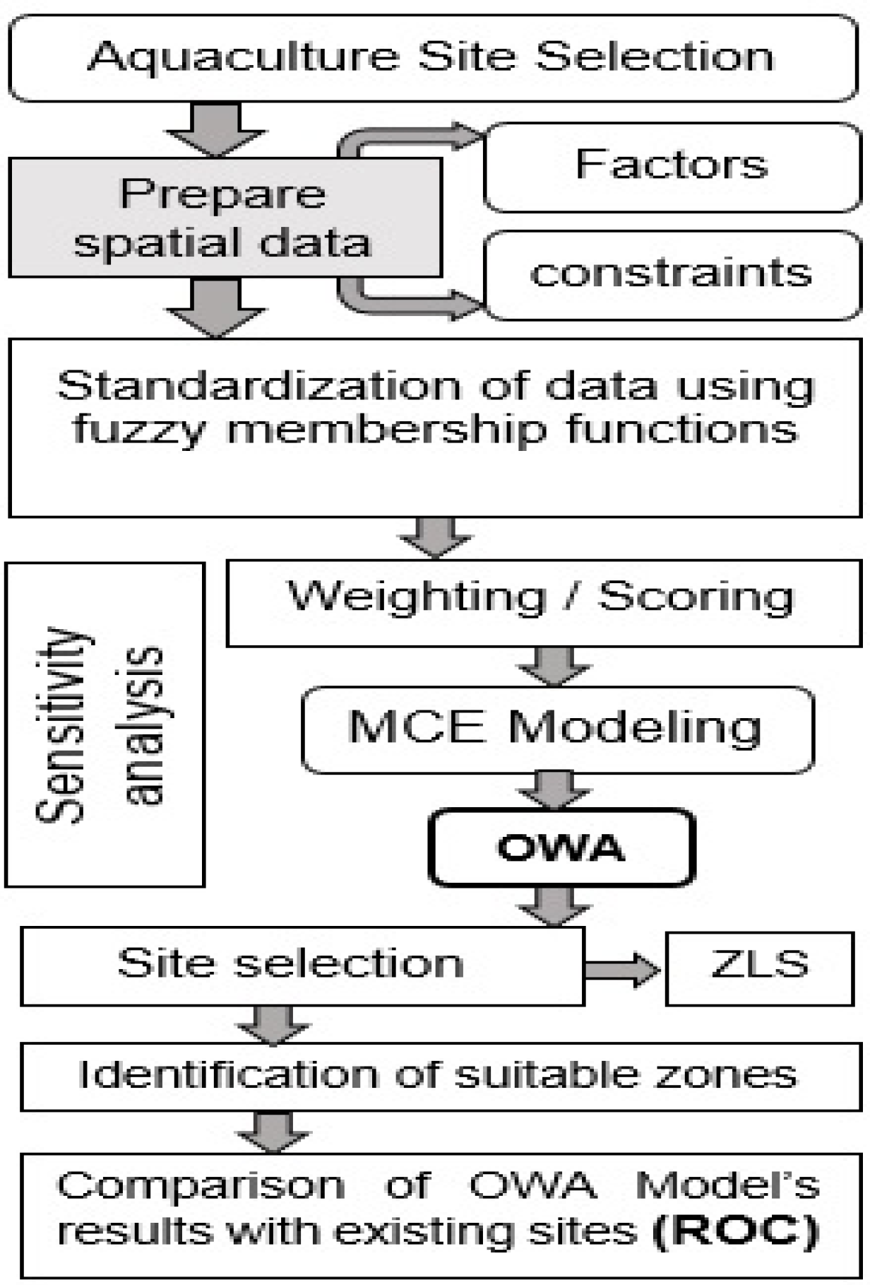
2. Materials and Methods

2.1. Case Study Specification

The Caspian Sea is the largest lake on Earth with no outlets. Its area is divided into three, approximately equal, parts: Northern, Middle, and Southern. The Southern Caspian has the largest volume, some 64% of the total volume, and its area is 35% of the total area of the sea. It is the deepest part of the sea, with a maximum depth reaching 1025 m [27]. The mean salinity of the Caspian Sea equals 12.85 g/L. The salinity of the Southern Caspian is 13 g/L. Water temperature in the Southern parts of the Caspian Sea never falls below 13 °C in winter and increases up to 25 or even 30 °C in summer [28]. The study area included the Coasts of Mazandaran Province in the south of the Caspian Sea to the depth of 50 m in 35047′ and 38005′ N and 50034′ and 56014′ E (Figure 1). The coastline length in the southern part of the Caspian Sea is 873 km (Mazandaran Province coastline: 487 km). The coastline is relatively smooth. There are no bays or capes that are considered the best locations for cage culture.

2.2. Identification, Obtaining, and Preparing the Environmental Criteria and Spatial Database Acquisition

The conceptual structure of the spatial analysis method for the selection of suitable sites for marine aquaculture operations is illustrated in Figure 2. In Table 1, the main factors and constraints by their sources are mentioned. This study identified 18 criteria according to the basic requisite for Rainbow trout (Oncorhynchus mykiss) aquaculture in Mazandaran Province, southern part of the Caspian Sea. These criteria were organized into three submodels (Physical–Environmental, Social–Economic, and Water Quality) and constraints (Harbor, River mouth, Bathometry, Distance from the coastline) represented either as factors or constraints (Nath et al., 2000). Identification, acquisition, and normalizing the criteria are the first steps in the conceptual structure. The second step requires one or more decision-makers to determine the weight of their criteria and ORness values for the calculation of order weights. The ORness value reveals the risk level in the decision-making process [29]. The GIS-based OWA model was used in the third step to utilize the criteria and decision-makers’ priorities for the development of suitable areas for marine aquaculture. Finally, to verify the suitability of the final model outputs, comparisons were made between the predicted suitable sites and existing farm locations.

2.2.1. Water Quality Parameters: Sea Surface Temperature

Data for sea surface temperature (SST) were obtained using a Moderate Resolution Imaging Spectroradiometer (MODIS)-Aqua sensor with a resolution of 4 km, provided by the Distribution Active Archive Centre Goddard Space Flight Centre National Aeronautics and Space Administration (DAAC/GSFC/NASA). Monthly data was obtained for the period of 2010 to 2015. Then, the 72 images obtained were processed from the maximum and minimum SST image (Figure 3).

2.2.2. Water Quality Parameter: Suspended Solids

A high correlation between suspended solids and the normalized water-leaving radiance at 555 nm, nLw (555), has been observed in several studies [30,31]. Therefore, we used the nLw (555) as a proxy of the concentration of suspended solids. The nLw (555) values were obtained from MODIS images. Monthly data were collected between 2010 and 2015. All images were combined to generate a single image, which was used to generate average values of suspended solid (Figure 4).

2.2.3. Water Quality Parameter: Chlorophyll-a

Phytoplankton is food for many fish species, but the high amount of phytoplankton is also an indication of eutrophication. The concentration of chlorophyll-a is often used as a proxy to describe phytoplankton biomass. In various studies, chlorophyll-a is considered an important factor in site selection for marine aquaculture [31]. MODIS data at 4 km resolution imagery was used in the analysis. The chlorophyll-a product using the OC4 algorithm was utilized. Monthly data were collected from 2010 to 2015. The images were combined into a single image to obtain average values of chlorophyll-a concentration (Figure 5).

2.2.4. Physical–Environmental Parameter: Bathymetry

The fish cages have to be located in regions where the water depth is sufficient. This allows avoiding harmful feedback from the accumulation of waste material [9]. According to this criterion, the depth of 30 to 50 m was chosen as the most suitable depth for marine aquaculture development. Bathymetry lines in the Southern Caspian Sea were installed by the Iranian National Cartographic Center Using GIS (10.2) software and by the raster function to produce raster format images (Figure 6).

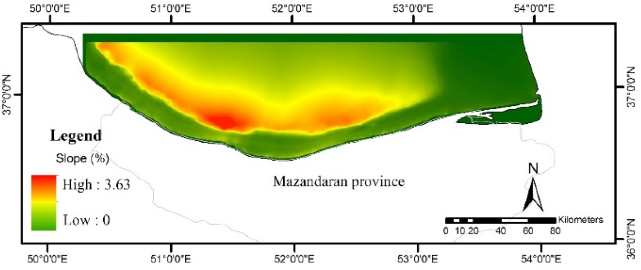
2.2.5. Physical–Environmental Parameter: Slope of Seabed

Farm construction and cage drainage could be affected by the bottom slope of the area. The slope of Seabed (%) was obtained from the bathymetry image such that the Bathymetry raster image was divided into distance to beach image [23,31] (Figure 7).

2.2.6. Physical–Environmental Parameter: Maximum Wave Height and Wind Speed

The maximum wave height and wind speed may incur cage damage, cause stress on structures, and make an environment unsafe for operators [24,25,32]. Therefore, these two parameters have to be considered when making decisions about the locations of fish farms. The modified operational wind field of European Centre for Medium-Range Weather Forecasts (ECMWF) and the national project called ISWM (Iranian Seas Wave Modeling) from 1992 to 2002 were used as the best available data source in this study. Maximum wind speed and wave height in a 12-year period for the depth zone between 20 to 50 m is shown in Figure 8.

2.2.7. Physical–Environmental Parameter: Current Velocity

High current velocity affects both the physical structure of the cages by incurring torsional forces on the netting, fatigue, and fracture on couplings and welding points and also the fish production and behavior by deforming the nets, oxygen supply, or waste clearance, and even causing excessive forced swimming [33]. To this purpose, current velocity simulation results have been used by the Hybrid-Coordinate Ocean Model (HYCOM) model for the Caspian Sea [34]. According to this model, current velocity was obtained in two directions of U and V. Finally, current velocity was provided using Equation (1). Figure 9 shows the maximum current velocity of sea-level in the case study.
V   =   v 2 + u 2

2.2.8. Social–Economic Parameters

There are also several socio-economic criteria that affect fish farming (such as distance from the coastline, distance to industries, distance to tourist areas, distance to cities, distance to coastal protected areas) because new development will be constrained by current land use and cannot occur on already developed land. Figure 10 illustrates them in the southern part of the Caspian Sea.

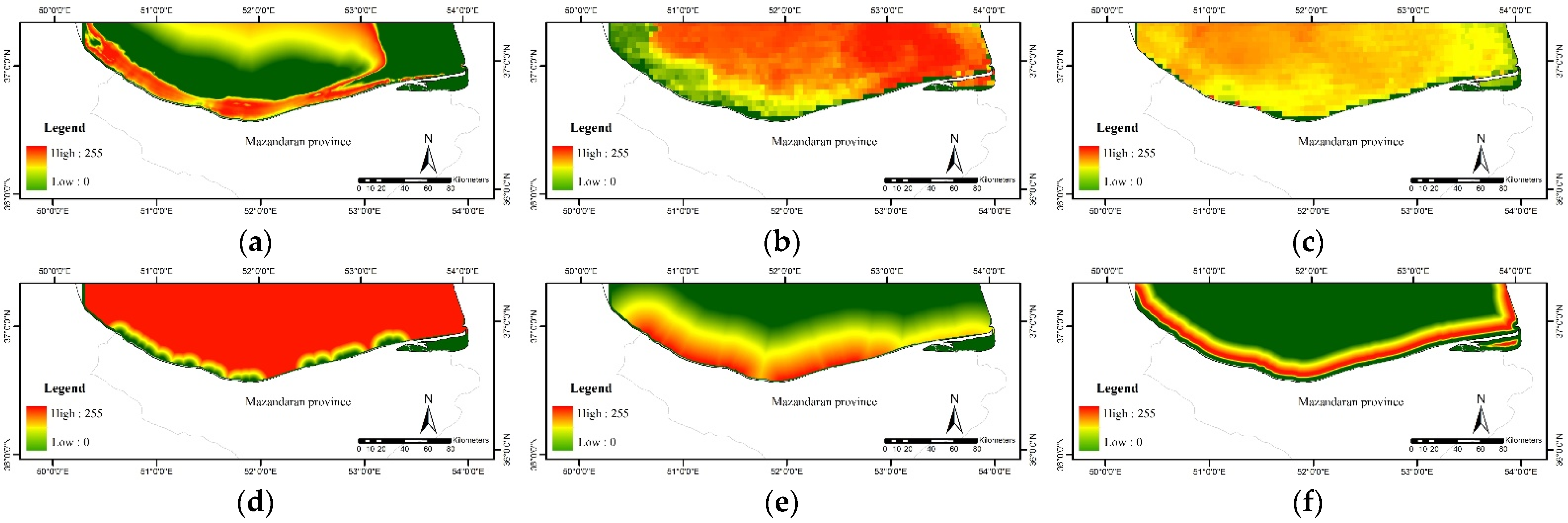
2.3. Standardization and Priority Weighting of Criteria

All criteria were standardized in a range of 0–255 (255 high suitability) using fuzzy membership functions in TerrSet software that is based on maximization or minimization of the attribute. The choice of function and control points based on expert opinions of the research team and literature, the shape of the suitability curve, and the control points are shown in Table 2.
The next stage was to establish a weighting for each criterion and factor, where a weight is assigned to each factor to express the importance of every variable in relation to others, and the pairwise comparison method of the Analytical Hierarchy Process (AHP) was used to determine the weight of the factors (standardized criteria) by priority [35]. The weighting of the factors was done according to the optimal growth under farm conditions and was judged by experts. Moreover, the consistency ratio (CR) of the matrix was calculated, which indicates the probability that ratings are assigned in a random manner. A consistency ratio of 0.10 or less was considered acceptable [36]. Table 3, Table 4 and Table 5 show the obtained criterion weights. In this stage for each category (Physical–Environmental; Social–Economic; Water Quality), a separate multi-criteria evaluation model was implemented and then the outputs of each group were imported in another multi-criteria evaluation model (final model).

2.4. GIS-Based Multi-Criteria Evaluation (MCE) with Ordered Weighted Averaging (OWA) Method
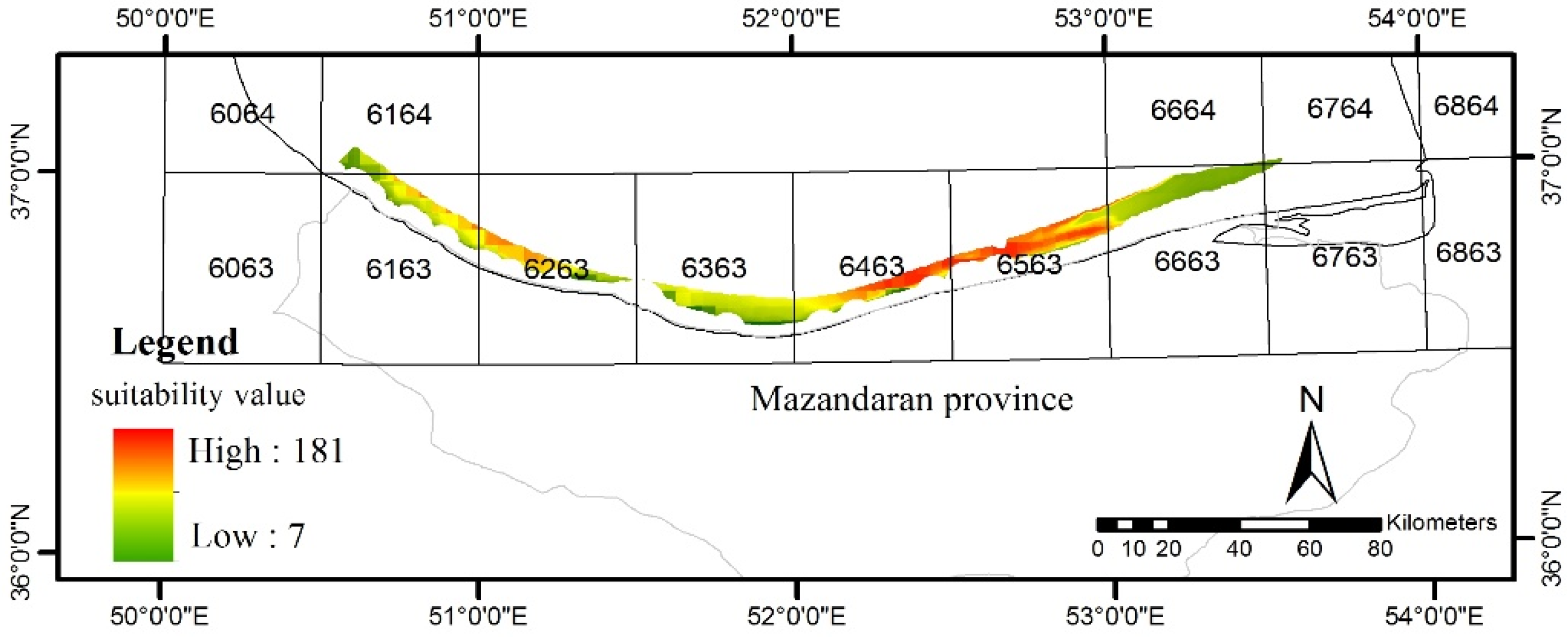
Ordered Weighted Averaging (OWA) makes use of a group of multi-criteria operators and two sets of weights: criterion or relevance weights and order weights. By using OWA, a range of weighting designs were modeled to control the decision risk in the determination of the factors affecting the aquaculture site suitability [37]. Considering a set of n criteria, an OWA operator can be defined as the function F: In → I with a related set of order weights V = [v1, v2, … , vn]; vj∈ [0, 1] for j = 1, 2, … , n and j = 1 n v j = 1 . Considering the set of standardized attribute values Ai = [ai1, ai2, … ,ain] for i = 1, 2, … , m, in which aij ∈ [0, 1] constitutes the j-th attribute related to the i-th location, the OWA operator will be defined as follows.
O W A i ( a i 1 , a i 2 , a i 3 , a i n ) = j = 1 n v j z i j
where zi1zi2 ≥ … ≥ zin is the sequence which is obtained by reordering the attribute values ai1, ai2,…,ain. The reordering process is a determining factor for the OWA operator and involves a weight, vj, with a predetermined ordered position of the attribute values ai1, ai2,…,ain for the i-th location. The first order weight, v1, is assigned to the highest attribute value for the i-th location, v2 is assigned to the second-highest value for the same location, and so on; and finally, vn is assigned to the lowest attribute value. It is important to note that a particular value of aij is not related to a particular weight vj, but rather the weight is assigned to a particular ordered position aij. The generality of OWA is due to the fact that by selecting the appropriate order weights, it is able to provide a wide range of map combination operators [29]. OWA operators can be characterized by two features; the first of which is the attitudinal character (ORness). The ORness represents the risk level of factor attribute misinterpretations (on a scale of 0 to 1). This characterizes emphasis on better and worse values and shows the degree of risk in decision-making, and can be achieved through Equation (3). The more the amount of ORness, the higher will be the amount of risk-taking and vice versa. Another measure in operation OWA is ANDness which is defined in Equation (4) [35,38].
ORness = 1 ( 1 n 1 r ( n 1 ) w r )
A N D n e s s = 1 ORness
where n is the number of factors, r is the order of factors, and wr is the weight for the factor of the rth order.
The second feature by which the OWA operators can be characterized is the degree of dispersion (tradeoff). On a scale of 0–1, the tradeoff represents the level by which the good performance of one factor can be substituted with the poor performance of another (compensation). The tradeoff feature can be obtained by using Equation (5).
T R A D E O F F = 1 n r ( w r 1 / n ) 2 n 1
where n is the number of factors, r is the order of factors, and Wr is the weight for the rth order factor. The Tradeoff is dependent on the weights that are distributed across all factors used in a weighting combination [37]. Table 6 indicates the calculated values for ORness, ANDness, and Trade-off in this study.
The risk level to be assumed in the MCE can be controlled by using OWA. Furthermore, the degree to which factor weights (trade-off) will affect the final suitability map OWA, which will provide us with a range of possible solutions for our aquaculture sites problem. In this case, 14 order weights corresponding to the 14 factors which were rank-ordered for each site were used after the application of the modified factor weights. Six typical sets of order weights for the 14 factors are shown in Table 6: (a) average level of risk and full trade-off, (b) low level of risk and no trade-off, (c) high level of risk and no tradeoff, (d) low level of risk and average trade-off, (e) high level of risk and average trade-off, (f) average level of risk and trade-off. Illustrated in Figure 11 are the locations of typical sets of order weights in the decision–support space [39].

2.5. Site Selection

In order to select the most appropriate sites, ZLS (Zonal Land Suitability) method [40] was used based on a minimum suitability threshold and minimum area that the FASI (Final Aggregated Suitability Image) layers in each of six typical sets of order weights were grouped into several zones. Then, zones were ranked in descending order by using Equation (6).
S z = ( ( L i ) z n z )
where Sz is the ZLS of each zone, (Li)z is the local suitability of the cell Si which belongs to zone z, and nz indicates the number of cells in zone z.
In this study, it was stipulated that a minimum score of 200 for suitability and 10 ha of area are required for a cage culture (Source: Iranian Fisheries Organization). Therefore, zones less than 10 hectares were deleted from the final suitability areas.

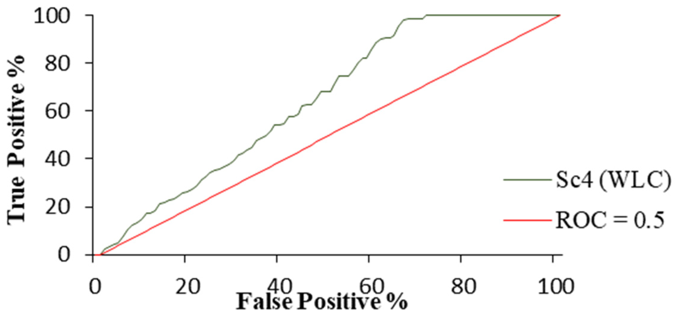
2.6. Comparison of OWA Model’s Results with Existing Sites (ROC)

Comparisons were made between the predicted suitable sites and existing farm locations to verify the suitability of final model outputs. In this study, accuracy assessment was used on ROC (Relative Operating Characteristic) Statistics [41]. In order to assess the validity of a model that predicts the location of the occurrence of a class by comparison of a suitability image depicting the likelihood of class occurring (i.e., the input image), ROC represents a very promising method. In the present study, where that class actually exists, is determined by the Boolean image (i.e., the reference image). The ROC is defined in the range of 0 to 1 [41].

2.7. Sensitivity Analysis

In the sensitivity analysis, the most important element to be considered is weight because weights are the basis of value judgments and include a subjective number about which decision-makers may disagree. In this study, the sensitivity analysis was aimed at investigating the sensitivity of the weights of various criteria on the spatial pattern of site suitability. Sensitivity analysis was made by increasing each parameter by a given percentage while keeping the others constant in quantifying the change in the model output. Intervals of ±5%, ±10%, and ±20% were chosen for the reference values. Suitability maps for every interval were created. The change of areas under the suitability score of every weighting scheme was investigated. The output map of each scenario with the base map) FASI of scenario a) was compared through relationships between image difference (9), percentage change (10), and ratio image (11) [42]. In addition, Cramer’s V coefficient was used to investigate the correlation between the criteria and suitable sites for aquaculture. In total, it was discovered that the variables with a Cramer’s V of about 0.15 or higher were considered useful while those with values of 0.4 or higher were good [43].
Image difference = Second image − First image
Percentage   Change   =   Second   image   First   image   First   image × 100
Ratio   Image   =   Second   image First   image  

3. Results

This section may be divided by subheadings. It should provide a concise and precise description of the experimental results, their interpretation, as well as the experimental conclusions that can be drawn.

3.1. Standardization and Priority Weighting of Criteria

Every constraint was acquired as a Boolean map while fuzzy membership functions were used to standardize the factors. The standardized results of all 18 factors and the constraints for marine aquaculture are shown in Figure 12.
Then, using the Extract function, the average value of each parameter and also the amount of utility (fuzzy number) in all 9 available farms were calculated. The results of this function are shown in Table 7.

3.2. GIS-Based Multi-Criteria Evaluation (MCE) with Ordered Weighted Averaging (OWA) Technique

The OWA combination procedure aims at the identification and prioritization of areas on the coasts of Mazandaran Province (depth of 20 to 50 m) for marine aquaculture. Five decision strategies were deployed in the present study. Each strategy is related to a specified value of ORness and the relationship between tradeoff and Risk (Figure 11, Table 6). OWA allows the control of the MCE status in both the risk and the tradeoff. In other words, it permits the control of the risk level assumed in the proposed MCE, and the effects of factor weights (tradeoff weights) on the final suitability map (Figure 11). The OWA weights which are shown in Table 6 were used to make various scenarios to control the trade-off and risk levels. These scenarios are as follows:
Scenario a
In this scenario, the risk level is between AND and OR; and the level of tradeoff is full. Consequently, and based on Table 6, the following order weights are specified. Here, weight is distributed or dispersed evenly among all factors without taking into account their rank-order position from minimum to maximum for any given location. This scenario is similar to the WLC method (Figure 13).
Scenario b
In this scenario, full weight assigned to the first rank-order results (the minimum suitability score among all factors for every pixel) will be the same as the AND operation in Boolean MCE. Here, full weight is assigned to the factor with the minimum value. The order weights used for AND operation are shown in Table 6. In addition, such weighting leads to conditions with no tradeoff and low risk (Figure 14).
Scenario c
In this scenario, full weight assigned to the last rank-order results (the maximum suitability score in all factors for each pixel) will be exactly the same as the OR operation in MCE. The order weights used for OR operation are shown in Table 6. Moreover, such a weighting technique results in no tradeoff and high risk (Figure 15).
Scenario d
In this scenario, for example, stakeholders and managers may be interested in a conservative or low-risk solution for identifying suitable areas for marine aquaculture. However, they also know that their estimates for how different factors should tradeoff with one another are important and should be taken into consideration as well. Then, a set of order weights that provides some tradeoff but maintains a low level of risk in the solution will be generated. Several sets of order weights exist that could be applied to achieve this. For low risk, the weight should be skewed to the minimum end. For some tradeoffs, weights are to be distributed across all ranks. The set of order weights is shown in Table 6 and the results of this scenario have been illustrated in Figure 16.
Scenario e
In this scenario, these order weights determine an operation that takes place midway between the extremes of AND and the average risk position of WLC. Furthermore, these order weights set the level of tradeoff midway between the no tradeoff situation of the AND operation and the full tradeoff situation of WLC (Figure 17).
Scenario f
In this scenario, the risk level is exactly between AND and OR and the tradeoff level is average (Table 6). Figure 18 shows the results of this scenario.

3.3. Site Selection

The results of the application of the ZLS methodology for 3 scenarios a, b, and d are presented in Figure 19. The zones are then ranked in descending order by the value of their zonal land suitability to facilitate the decision process. According to available reports of the Iranian Fisheries Organization, studies done for marine aquaculture site selection in the south of the Caspian Sea are applied by the weighted linear combination (WLC). The risk of this scenario is 50%. Since the fish culture in cages includes high-risk activities, models and methods should be used to determine the appropriate location with the least environmental damage. Three scenarios a, b, and d are important environmental scenarios with low risk. The more scenario b (AND) moves toward scenario c (OR), the more the amount of suitability and the number of the appropriate zone increases. Accordingly, scenarios a, b, and d were, respectively, introduced to zones 4, 8, and 11 as the end zones in each scenario. Nevertheless, scenarios e, c, and f have high-risk so they do not have favorable results.
Then, using the Extract function, the average value of each parameter and also the amount of utility (fuzzy number) in each of the 9 available farms were calculated. The results of this function are shown in Table 8.

3.4. Comparison of OWA Model’s Results with Existing Sites (ROC)

ROC is a summary of statistics obtained by several two-by-two contingency tables, based on a comparison of the simulated and reference images. In this study, simulated image was the Final Aggregated Suitability Image (FASI) of scenario a (WLC) and the reference image was existing aquaculture farms (9 farms) on the coasts of Mazandaran Province. In Figure 20, the amount of ROC was calculated as 0.69 and this showed that aquaculture sites in the coastal of Mazandaran province were selected correctly based on weighted linear combination method but according to the ROC (0.69), the position of these farms can still be transferred to areas more suitable with less risk.

3.5. Results of Sensitivity Analysis

Table 9 shows the differences with the baseline model for each variable and every suitability score. Based on these results, an evaluation was made for the sensitivity of the models to the variations in the input parameters. Significant differences existed between the mean difference, percentage change, and ratio images in each scenario. The results of the sensitivity analysis in Table 9 showed that most of the parameters affecting the output location for marine aquaculture in the region were as follows: socioeconomic factors, water quality, and physical–environmental parameters. The model was more sensitive to lower than higher values of the parameters.
As noted in Section 2.7, Cramer’s V coefficient was used to evaluate the correlation between the criteria and suitable sites for aquaculture. Figure 21 shows Cramer’s V coefficient values for each parameter. According to the figure, bathymetry and distance from the coastline were the most effective parameters and maximum temperature had the least impact on site selection of marine aquaculture in the coastal areas of Mazandaran Province.

4. Discussion

This study investigated the potential use of Ordered Weighted Average (OWA) for marine aquaculture site selection. Many factors affect marine aquaculture, including water quality, physical-environmental, and socioeconomic factors. Here, 18 criteria were simultaneously considered to allow the decision-makers to figure out the effects of every criterion in the operations of a marine aquaculture farm. Therefore, each criterion was standardized using fuzzy membership functions with regard to the desirable criteria for fish culture.
The fuzzy image for maximum temperature shows, the indexes of the east coast (as illustrated in Figure 1) are less desirable for fish farming than the west coast due to higher temperature and the temperature increases from the west to the east. Furthermore, the lowest suitability was obtained in indexes 6664 and 6763 by amounts of 45 and 43, and the most suitability was in indexes 6164 and 6263 by amounts of 198 and 191. Fuzzy picture of chlorophyll-a showed that the fuzzy number in index 6763 was equal to 56, which is an indication of high chlorophyll content and low utility value in this area. Gentle slope of the seabed and slower current velocity in Gorgan Bay and Miankaleh can cause high levels of chlorophyll in this area.
For socio-economic factors, increasing and decreasing Liner functions were used because there is a direct relationship between the distance factor and fuzzy number. In distance from the coastline factor, indexes 6663, 6763, and 6767 had the lowest suitability levels of 37, 49, and 46, respectively, since the suitable depth was in a farther distance from the coastline in the east.
Wave height and wind speed factors were standardized by using S-shaped function and the three factors of seabed slope, bathymetry, and current velocity were standardized by linear symmetric function in physical and environmental submodule. In bathymetry, a fuzzy image in indexes 6764 and 6763 had the lowest utility levels of 45 and 62. Bathymetry results correspond with the results of distance to the coastline and seabed slope. The maximum amount of wave height and wind speed were, respectively, 4 to 5 m and 16 to 27 m/s according to the studies by References [26,33]. The east and west coast indexes had less suitability since the wave height and wind speed were more than optimal in central indexes 6263, 6364, and 6463. Based on previous studies, the optimal seabed slope for marine aquaculture was 0.5% to 2% [16,25,26]. In indexes 6663, 6664, 6763, and 6764, the seabed slope was less than 0.2% on the east coast and Gorgan Bay and it began to increase toward the west coast. In this paper, the weight has been done on the basis of the review of past studies. According to Table 5, among water quality factors, most weights were assigned to the temperature. Several studies such as the study of Pérez et al., 2005, and the other studies [16,31] showed that water temperature has the highest value among environmental factors. Among the socio-economic factors, more amounts of weight were dedicated to factors such as distance from industrial areas, distance from tourist areas, distance from the coastline, distance from the protected areas, and distance from the city with the values of 0.31, 0.28, 0.19, 0.13, and 0.07 [16,23,25]. Among the physical–environmental factors, more amounts of weight were dedicated to factors such as seabed slope, bathymetry, wave height, wind speed, and current velocity with the values of 0.31, 0.25, 0.20, 0.12, and 0.09.
One of the major barriers in site-selection analyses using multi-criteria evaluation procedures is weighting. Weightings should be in accordance with the priorities of decision-makers as far as possible [44]. After the weights are assigned, a sensitivity analysis should be performed to investigate their effects on the overall results. In this study, when parameters contained varied weights, significant changes were observed in terms of suitable aquaculture areas. Most of the parameters affecting the output location of marine aquaculture in the region were, respectively, as follows: social-economic, water quality, and physical–environmental parameters; and the model was more sensitive to lower than higher values of the parameters.
Not only was the weight of each factor used but also the OWA weights which are shown in Table 6 were used to generate various patterns to address the trade-off and risk levels. Scenario b or AND is related to the AND operator and provides a risk averse solution. Based on this scenario, the most suitable areas for marine aquaculture are located in indexes 6163, 6463, and 6563 (Figure 19a). The legends in Figure 14 indicate a measure of aquaculture suitability in which the possibility ranged on a scale between 1 and 68. The value of 1 for the ANDness in Table 6 reveals that the solution is coincident with the AND while the value of 0 for the ORness shows that the solution is the most distant from OR. The trade-off measure of zero indicates no trade-off.
Scenario d increases the risk level and provides an area suitable for marine aquaculture. In Table 6, the value of 0.64 is shown for the ANDness while the value of 0.36 is presented for the ORness and this solution pattern allows a trade-off equal to 0.47. This scenario is midway between AND and the conventional weighted linear combination (WLC) in triangular decision space. The suitability for aquaculture, as shown in Figure 16, increased compared to scenario a. The legends in Figure 16 indicate a measure of aquaculture suitability in which possibility ranged between 181 and 7. Considering the ZLS results provided for this scenario, the most suitable areas for marine aquaculture site-selection are located on indexes 6163, 6263, 6463, and 6563 (Figure 19b).
Scenario a (WLC) and f (AVG) are in the middle of the risk continuum which is neither risk averse nor risk-taking solutions. The slight difference between the AVG and WLC solutions is that trade-offs are allowed in the former (Table 6). Figure 13 and Figure 18, by comparing the corresponding maps, suggest that scenario f produces a larger area for marine aquaculture. Based on scenario a, the most desirable areas for marine aquaculture are located on indexes 6163, 6164, 6363, 6463, and 6563 (Figure 20c). In Table 6, with the value of 0.5 for the ANDness and the ORness, also this solution pattern allows a trade-off equal to 1 for scenario a (WLC).
According to Figure 17, Scenario e falls between the WLC and the OR, in which trade-offs are allowed to some extent, and scenario c (OR) (Figure 15) is in the opposite extreme from the AND solution. A very large spatial extent could be assigned to the suitable areas for marine aquaculture with this alternative which includes all of the areas. Finally, the OR solution is observed at the extreme of the continuum, which suggests almost the entire area as suitable for aquaculture (Figure 15 and Figure 17).
Since the fish culture in cages includes high-risk activities, models and methods should be used to determine the appropriate location that has the least environmental damage. So, scenarios c and e have high-risk and do not have a good result. The legends in Figure 15 indicate a measure of aquaculture suitability in which possibility ranges between 247 and 255. In Table 6, the value of 0 for the ANDness suggests that the solution is coincident with the OR while the value of 1 for the ORness suggests that the solution is the most distant from AND. The trade-off measure of 1 indicates no trade-off.

Evaluating and Comparing the Existing Aquaculture Farms and Selected Sites in the Area of Study

It is necessary that the average value and the suitability (fuzzy number) for each parameter are determined in every 9 existing farms and 11 selected sites in order to evaluate and analyze the existing aquaculture farms on the coasts of Mazandaran Province. There is index 6563 in farm 1 and all parameters in this farm have good condition and fuzzy number, except the bathymetry factor in other factors is more than 100. It is recommended that the location of farm 1 is transferred away from the coastline to a more appropriate bathymetry.
Farm 2 is on the coast of Babolsar in index 6563. Based on all the parameters, it has a favorable situation but this farm is near two landfills in Fereydoon Kenar and Babolsar, so the fuzzy number in distance to industry factor is 74. The location of farm 2 should be transferred away from the coastline to a more appropriate bathymetry.
Farm 3 is on the coast of Noshahr in index 6363. Fuzzy number for distance to coastal protected factor is of the lowest amount of 12. This farm is located 7 km from Alborz protected area. In addition, the current velocity and minimum temperature factors are lower than the standard level. In this farm, the amounts of these two factors for current velocity and minimum temperature are, respectively, equal to 0.06 m/s and 7.6 °C.
Two farms 4 and 9 in indexes 6363 and 6163 in OWA have various scenarios because based on constraints images, farm 4 is located in Noshahr harbor scope and farm 9 in Ramras harbor protected scope, with a value of zero.
Farms 5 and 6 are located in Chaluos and Tonekabon coastal areas (index 6263). The suitability of the minimum temperature factor is low. In addition, socio-economic factors in this index have very low suitability.
Farms 7 and 8 are located on the coast of Tonekabon in indexes 6263 and 6163. Both farms in all parameters have low suitability except the suspended solid and distance to industry factor. According to what was mentioned, farms 1 and 2 have the best situation and the highest suitability.

5. Conclusions

An important factor for successful marine aquaculture and for the sustainable development of the industry is proper site selection. The present paper proposes the OWA methodology as a site selection technique for fish culture along the coasts of Mazandaran Province. A robust interactive toolset is provided by the OWA approach for adjusting trade-offs and compensation between criteria which makes possible a rapid investigation and interpretation of alternative scenarios and relationships between criteria. Other advantages of this approach are: the ability to integrate heterogeneous datasets such as quantitative and qualitative criteria using expert opinion, criteria selection flexibility for different study areas or different problems under consideration, implementation of one or more decisions, the flexibility to change the relevance level of criteria, and the freedom in the development of several modeling scenarios for acceptable levels of decision risks. Since the fish culture in cages is a high-risk activity, this methodology has been shown to have a significant potential to shed the decision-making complexities in real-world applications.

Author Contributions

Conceptualization, M.G.; methodology, M.G.; software, E.H. and M.G.; validation, M.G., N.M., and T.K.; formal analysis, E.H; investigation, E.H; resources, E.H.; data curation, E.H.; writing—original draft preparation, E.H.; writing—review and editing, M.G. and T.K.; visualization, E.H.; supervision, M.G.; project administration, M.G; funding acquisition, T.K. All authors have read and agreed to the published version of the manuscript.

Funding

The authors extend their appreciation for the support provided by the authorities of the Tarbiat Modares University in funding the study.

Institutional Review Board Statement

Not applicable.

Informed Consent Statement

Not applicable.

Data Availability Statement

Not applicable.

Acknowledgments

The study presented here is part of the thesis in partial fulfillment of the requirements for the degree of M.Sc. in Tarbiat Modarres University (T.M.U.) of Iran. Tiit Kutser’s work was supported by the Estonian Research Council grant PRG302.

Conflicts of Interest

The authors declare that there is no conflict of interest.

References

  1. Asche, F. Farming the sea. Mar. Resour. Econ. 2008, 23, 527–547. [Google Scholar] [CrossRef]
  2. Lucas, J.S.; Southgate, P.C. Reproduction, Life Cycles and Growth. Aquaculture: Farming Aquatic Animals and Plants; John Wiley & Sons: Hoboken, NJ, USA, 2019; pp. 113–126. ISBN 978-1-119-23086-1. [Google Scholar]
  3. Godfray, H.C.J.; Beddington, J.R.; Crute, I.R.; Haddad, L.; Lawrence, D.; Muir, J.F.; Toulmin, C. Food security: The challenge of feeding 9 billion people. Science 2010, 327, 812–818. [Google Scholar] [CrossRef] [PubMed] [Green Version]
  4. FAO. Food and Agriculture Organization of the United Nations. The State of World Fisheries and Aquaculture; FAO: Rome, Italy, 2014; p. 223. Available online: http://www.fao.org/3/a-i3720e.pdf (accessed on 30 September 2015).
  5. FAO. Food and Agriculture Organization of the United Nations. The State of World Fisheries and Aquaculture; FAO: Rome, Italy, 2020; p. 224. Available online: http://www.fao.org/3/ca9229en/ca9229en.pdf (accessed on 30 August 2020).
  6. Christie, N.; Smyth, K.; Barnes, R.; Elliott, M. Co-location of activities and designations: A means of solving or creating problems in marine spatial planning? Mar. Policy 2014, 43, 254–261. [Google Scholar] [CrossRef]
  7. Afroz, T.; Alam, S. Sustainable shrimp farming in Bangladesh: A quest for an Integrated Coastal Zone Management. Ocean Coast. Manag. 2013, 71, 275–283. [Google Scholar] [CrossRef]
  8. Suplicy, F.M.; Vianna, L.F.D.N.; Rupp, G.S.; Novaes, A.L.; Garbossa, L.H.; de Souza, R.V.; dos Santos, A.A. Planning and management for sustainable coastal aquaculture development in Santa Catarina State, south Brazil. Rev. Aquac. 2017, 9, 107–124. [Google Scholar] [CrossRef]
  9. Pérez, O.M.; Ross, L.G.; Telfer, T.C.; del Campo Barquin, L.M. Water quality requirements for marine fish cage site selection in Tenerife (Canary Islands): Predictive modelling and analysis using GIS. Aquaculture 2003, 224, 51–68. [Google Scholar] [CrossRef]
  10. Cho, Y.; Lee, W.C.; Hong, S.; Kim, H.C.; Kim, J.B. GIS-based suitable site selection using habitat suitability index for oyster farms in Geoje-Hansan Bay, Korea. Ocean Coast. Manag. 2012, 56, 10–16. [Google Scholar] [CrossRef]
  11. Llorente, I.; Luna, L. The competitive advantages arising from different environmental conditions in seabream, Sparus aurata, production in the Mediterranean Sea. J. World Aquac. Soc. 2013, 44, 611–627. [Google Scholar] [CrossRef]
  12. Tammi, I.; Kalliola, R. Spatial MCDA in marine planning: Experiences from the Mediterranean and Baltic Seas. Mar. Policy 2014, 48, 73–83. [Google Scholar] [CrossRef]
  13. Perez, O.M.; Telfer, T.C.; Ross, L.G. Geographical information systems-based models for offshore floating marine fish cage aquaculture site selection in Tenerife, Canary Islands. Aquac. Res. 2005, 36, 946–961. [Google Scholar] [CrossRef]
  14. Corner, R.A.; Brooker, A.J.; Telfer, T.C.; Ross, L.G. A fully integrated GIS-based model of particulate waste distribution from marine fish-cage sites. Aquaculture 2006, 258, 299–311. [Google Scholar] [CrossRef]
  15. Longdill, P.C.; Healy, T.R.; Black, K.P. An integrated GIS approach for sustainable aquaculture management area site selection. Ocean Coast. Manag. 2008, 51, 612–624. [Google Scholar] [CrossRef]
  16. Radiarta, I.N.; Saitoh, S.I. Satellite-derived measurements of spatial and temporal chlorophyll-a variability in Funka Bay, southwestern Hokkaido, Japan. Estuar. Coast. Shelf Sci. 2008, 79, 400–408. [Google Scholar] [CrossRef]
  17. Kamruzzaman, M.; Baker, D. Will the application of spatial multi criteria evaluation technique enhance the quality of decision-making to resolve boundary conflicts in the Philippines? Land Use Policy 2013, 34, 11–26. [Google Scholar] [CrossRef] [Green Version]
  18. Krois, J.; Schulte, A. GIS-based multi-criteria evaluation to identify potential sites for soil and water conservation techniques in the Ronquillo watershed, northern Peru. Appl. Geogr. 2014, 51, 131–142. [Google Scholar] [CrossRef]
  19. Nayak, A.K.; Pant, D. GIS-based aquaculture site suitability study using multi-criteria evaluation approach. Indian J. Fish. 2014, 61, 108–112. [Google Scholar]
  20. Nath, S.S.; Bolte, J.P.; Ross, L.G.; Aguilar-Manjarrez, J. Applications of geographical information systems (GIS) for spatial decision support in aquaculture. Aquac. Eng. 2000, 23, 233–278. [Google Scholar] [CrossRef]
  21. Ross, L.G.; QM, E.M.; Beveridge, M.C.M. The application of geographical information systems to site selection for coastal aquaculture: An example based on salmonid cage culture. Aquaculture 1993, 112, 165–178. [Google Scholar] [CrossRef]
  22. Buitrago, J.; Rada, M.; Hernández, H.; Buitrago, E. A single-use site selection technique, using GIS, for aquaculture planning: Choosing locations for mangrove oyster raft culture in Margarita Island, Venezuela. Environ. Manag. 2005, 35, 544–556. [Google Scholar] [CrossRef] [PubMed]
  23. Liu, Y.; Saitoh, S.I.; Radiarta, I.N.; Isada, T.; Hirawake, T.; Mizuta, H.; Yasui, H. Improvement of an aquaculture site-selection model for Japanese kelp (Saccharina japonica) in southern Hokkaido, Japan: An application for the impacts of climate events. ICES J. Mar. Sci. 2013, 70, 1460–1470. [Google Scholar] [CrossRef] [Green Version]
  24. Gimpel, A.; Stelzenmüller, V.; Grote, B.; Buck, B.H.; Floeter, J.; Núñez-Riboni ITemming, A. A GIS modelling framework to evaluate marine spatial planning scenarios: Co-location of offshore wind farms and aquaculture in the German EEZ. Mar. Policy 2015, 55, 102–115. [Google Scholar] [CrossRef] [Green Version]
  25. Dapueto, G.; Massa, F.; Costa, S.; Cimoli, L.; Olivari, E.; Chiantore, M.; Povero, P. A spatial multi-criteria evaluation for site selection of offshore marine fish farm in the Ligurian Sea, Italy. Ocean Coast. Manag. 2015, 116, 64–77. [Google Scholar] [CrossRef]
  26. Falconer, L.; Telfer, T.C.; Ross, L.G. Investigation of a novel approach for aquaculture site selection. J. Environ. Manag. 2016, 181, 791–804. [Google Scholar] [CrossRef] [Green Version]
  27. Aladin, N.; Plotnikov, I.; The Caspian Sea. In Lake Basin Management Initiative, Thematic Paper. 2004. Available online: http://www.worldlakes.org/uploads/Caspian%20Sea%2028Jun04.pdf (accessed on 30 August 2017).
  28. Kostianoy, A.G.; Kosarev, A.N. The Caspian Sea Environment; Springer Science & Business Media: Berlin, Germany, 2005; Volume 5. [Google Scholar]
  29. Malczewski, J.; Rinner, C. Multicriteria Decision Analysis in Geographic Information Science; Springer: New York, NY, USA, 2015; p. 31. [Google Scholar]
  30. Nezlin, N.P.; DiGiacomo, P.M.; Stein, E.D.; Ackerman, D. Stormwater runoff plumes observed by SeaWiFS radiometer in the Southern California Bight. Remote Sens. Environ. 2005, 98, 494–510. [Google Scholar] [CrossRef]
  31. Radiarta, I.N.; Saitoh, S.I.; Yasui, H. Aquaculture site selection for Japanese kelp (Laminaria japonica) in southern Hokkaido, Japan, using satellite remote sensing and GIS-based models. ICES J. Mar. Sci. 2011, 68, 773–780. [Google Scholar] [CrossRef] [Green Version]
  32. Grant, J.; Bacher, C.; Ferreira, J.G.; Groom, S.; Morales, J.; Rodriguez-Benito, C.; Saitoh, S.I.; Sathyendranath, S.; Stuart, V. Remote sensing applications in marine aquaculture. Remote Sensing in Fisheries and Aquaculture, Rep. Int. Ocean Colour Coord. Group 2009, 8, 77–88. [Google Scholar]
  33. Falconer, L.; Hunter, D.C.; Scott, P.C.; Telfer, T.; Ross, L. Using physical environmental parameters and cage engineering design within GIS-based site suitability models for marine aquaculture. Aquac. Environ. Interact. 2013, 4, 223–237. [Google Scholar] [CrossRef] [Green Version]
  34. Kara, A.B.; Wallcraft, A.J.; Metzger, E.J.; Gunduz, M. Impacts of freshwater on the seasonal variations of surface salinity and circulation in the Caspian Sea. Cont. Shelf Res. 2010, 30, 1211–1225. [Google Scholar] [CrossRef]
  35. Gorsevski, P.V.; Donevska, K.R.; Mitrovski, C.D.; Frizado, J.P. Integrating multi-criteria evaluation techniques with geographic information systems for landfill site selection: A case study using ordered weighted average. Waste Manag. 2012, 32, 287–296. [Google Scholar] [CrossRef]
  36. Saaty, T.L. A scaling method for priorities in hierarchical structures. J. Math. Psychol. 1977, 15, 234–281. [Google Scholar] [CrossRef]
  37. Amiri, M.J.; Mahiny, A.S.; Hosseini, S.M.; Jalali, S.; Ezadkhasty, Z.; Karami, S. OWA analysis for ecological capability assessment in watersheds. Int. J. Environ. Res. 2013. [Google Scholar] [CrossRef]
  38. Kiavarz, M.; Jelokhani-Niaraki, M. Geothermal prospectivity mapping using GIS-based Ordered Weighted Averaging approach: A case study in Japan’s Akita and Iwate provinces. Geothermics 2017, 70, 295–304. [Google Scholar] [CrossRef]
  39. Yager, R.R. On ordered weighted averaging aggregation operators in multicriteria decisionmaking. IEEE Trans. Syst. Man Cybern. 1988, 18, 183–190. [Google Scholar] [CrossRef]
  40. Mahini, A.S.; Gholamalifard, M. Siting MSW landfills with a weighted linear combination methodology in a GIS environment. Int. J. Environ. Sci. Technol. 2006, 3, 435–445. [Google Scholar] [CrossRef] [Green Version]
  41. Eastman, R.J. IDRISI guid to GIS and Image processing. In Accessed in IDRISI Selva 17.00; Clark University: Worcester, MA, USA, 2012; p. 354. [Google Scholar]
  42. Eastman, J.R. TerrSet Manual System. In Accessed in TerrSet [18.10]; Clark University: Worcester, MA, USA, 2015; p. 392. [Google Scholar]
  43. KKumar, R.; Nandy, S.; Agarwal, R.; Kushwaha, S.P.S. Forest cover dynamics analysis and prediction modeling using logistic regression model. Ecol. Indic. 2014, 45, 444–455. [Google Scholar] [CrossRef]
  44. Butler, J.; Jia, J.; Dyer, J. Simulation techniques for the sensitivity analysis of multi-criteria decision models. Eur. J. Oper. Res. 1997, 103, 531–546. [Google Scholar] [CrossRef]
Figure 1. Location of the study area on the coast of Mazandaran Province, the southern part of the Caspian Sea, with the position of current aquaculture farms and geographic indexes.
Sustainability 13 02672 g001
Figure 2. Conceptual structure of GIS-Based OWA approach for developing marine aquaculture. (MCE: Multi-criteria evaluation; OWA: Ordered weighted average; ZLS: Zonal land suitability; ROC: Relative operating characteristics).
Sustainability 13 02672 g002
Figure 3. The minimum (a) and maximum (b) monthly mean temperatures (°C) in the Southern Caspian Sea from 2010 to 2015.
Sustainability 13 02672 g003
Figure 4. Average Rrs555 and nLw555 for the period between 2010 and 2015. (a): nLw555 (mWcm−2 μm−1 Sr−1), (b): Rrs555 (Sr−1). nLw555 = Rrs(555) × F0, F0 = MODIS nominal Band Solar Irradiances (= 183/76 Mw cm−2 μm−1).
Sustainability 13 02672 g004
Figure 5. Average chlorophyll-a in the southern part of the Caspian Sea for the period from 2010 to 2015.
Sustainability 13 02672 g005
Figure 6. (a): Hydrographic lines (b): Bathymetry raster image.
Sustainability 13 02672 g006
Figure 7. Slope of Seabed in the southern part of the Caspian Sea.
Sustainability 13 02672 g007
Figure 8. Maximum wind speed (m/s) (a) and wave height (m) (b) in a 12-year period (depth of 20 to 50 m).
Sustainability 13 02672 g008
Figure 9. Maximum current velocity (m/s) in the Caspian Sea according to the HYCOM model.
Sustainability 13 02672 g009
Figure 10. (a) Distance from the coastline; (b) Distance to industry; (c) Distance to tourist areas; (d) Distance to city; (e) Distance to coastal protected areas.
Sustainability 13 02672 g010
Figure 11. Decision–strategy space and typical sets of order weights (see Table 6).
Sustainability 13 02672 g011
Figure 12. Standardization of evaluation criteria. (a): Seabed Slope (b): Minimum Temperature (c): Maximum Temperature (d): Distance to industry (e): Distance to city (f): Distance from the coastline (g): Chlorophyll-a (h): Suspended solid (i): Distance to tourist areas (j): Maximum wind speed (k): Maximum wave height (l): Maximum wind speed (m): Bathymetry (n): Distance to coastal protected areas, (or): constraint maps ((o): Harbore, (p): Bathmetry (20 m>, 50 m<), (q): Distance from the coastline (3 km>, 20 km<), (r): the main river mouth) (unit of all maps is suitability).
Sustainability 13 02672 g012aSustainability 13 02672 g012b
Figure 13. Final aggregated suitability image (FASI) for scenario a.
Sustainability 13 02672 g013
Figure 14. Final aggregated suitability image (FASI) for scenario b.
Sustainability 13 02672 g014
Figure 15. Final aggregated suitability image (FASI) for scenario c.
Sustainability 13 02672 g015
Figure 16. Final aggregated suitability image (FASI) for scenario d.
Sustainability 13 02672 g016
Figure 17. Final aggregated suitability image (FASI) for the scenario e.
Sustainability 13 02672 g017
Figure 18. Final aggregated suitability image (FASI) for scenario f.
Sustainability 13 02672 g018
Figure 19. The final zones of site selection for scenarios: (a) AND, (b) MIDAND, (c) weighted linear combination (WLC).
Sustainability 13 02672 g019
Figure 20. ROC scenario of (WLC) with the existing aquaculture.
Sustainability 13 02672 g020
Figure 21. Cramer’s V coefficient for the criteria used in marine aquaculture site selection.
Sustainability 13 02672 g021
Table 1. Parameter requirements for Rainbow trout (Oncorhynchus mykiss) aquaculture development in the coasts of Mazandaran Province, the southern part of Caspian Sea, Iran.
Sub ModelsCriteriaUnitScale/ResolutionSources
(Water Quality)Temperature°C4 kmModerate Resolution Imaging
Spectroradiometer (MODIS)
Satellite, Aqua sensor
http://oceancolor.gsfc.nasa.gov accessed on 17 February 2021
(Maximum and minimum)
Suspended solidμm−1 Sr−1
Chlorophyll-aMg/m3
(Physical–Environmental)Bathymetry M1/25,000Iran National Cartographic Center
Maximum wave heightMIran Ports and Maritime Organization
(Iranian Seas Wave Modeling ISWM)
Maximum wind speedm/s
Slope Seabed%(Depth/distance of the beach) × 100
Maximum Current velocitym/s3 kmHYCOM Model, (Kara et al., 2010)
(Social–Economic)Distance to tourist areas m1/25,000Iran National Cartographic Center
Iran Department Environmental
Iran Ministry of Defence
Google Earth 7.1.5.1557
(Gholamalifard et al., 2012)
Distance to industry
Distance to beach
Distance to City
Distance to coastal protected areas
(Constrain)Harborm1/25,000
The main river mouth
Distance from the coastline (3–20 km)
Depth (20–50 m)
Table 2. The shape and type of fuzzy membership function with corresponding parameterization (start/endpoints) based for Rainbow trout on literature research and expert knowledge.
CriteriaControl PointsThe Shape and Type of Fuzzy Membership FunctionFunction EquationSource
Maximum Temperatureabcd
Liner and Symmetric Sustainability 13 02672 i001 X i = ( R i c d c ) × 255 [32]
20252530
Minimum TemperatureLiner and Symmetric Sustainability 13 02672 i002 X i = 1 ( R i a b a ) × 255
6101215
Suspended solidLiner and Monotonically decreasing Sustainability 13 02672 i003 X i = 1 ( R i a b a ) × 255 [16]
000.13.5
Chlorophyll-aSigmoidal and Monotonically decreasing Sustainability 13 02672 i004 μ = cos 2 α × 255
α = ( x c ) ( d c ) × p i 2
[11]
00010
Maximum wave heightSigmoidal and Monotonically decreasing Sustainability 13 02672 i005 [32]
0004
Maximum wind speedSigmoidal and Monotonically decreasing Sustainability 13 02672 i006 [33]
00027
Seabed SlopeLiner and Symmetric Sustainability 13 02672 i007 [25]
00.5110
Maximum Current velocityLiner and Symmetric Sustainability 13 02672 i008 [33]
0.020.150.20.3
BathymetryLiner and Symmetric Sustainability 13 02672 i009
03050100
Distance to industryLiner and Monotonically increasing Sustainability 13 02672 i010 X i = ( R i c d c ) × 255
012,00000
Distance from the coastlineLiner and Symmetric Sustainability 13 02672 i011
30005000750020,000
Distance to CityLiner and Monotonically decreasing Sustainability 13 02672 i012
0004500
Distance to coastal protectedLiner and Monotonically increasing Sustainability 13 02672 i013
050,00000
Distance to tourist areasLiner and Monotonically increasing Sustainability 13 02672 i014
0750000
Table 3. Pairwise comparison matrix for the analysis of the relevance of Physical–Environmental parameters.
(Weight: 0.3808)
Criteria(Bath)(SlS)(WH)(CV)(WS)Weight Criteria
(Bath) 11 0.2575
(SlS) 221 0.3183
(WH) 3½1/21 0.2011
(CV) 41/31/21/21 0.0956
(WS) 51/3½1/31/210.1275
CR = 0.03
1 Bathymetry, 2 Seabed Slope, 3 Maximum wave height, 4 Maximum Current velocity, 5 Maximum wind speed.
Table 4. Pairwise comparison matrix for the analysis of the relevance of Social–Economic parameters.
(Weight: 0.2158)
Criteria(DB)(DP)(DI)(DT)(DC)Weight Criteria
(DB) 11 0.1992
(DI) 1½1 0.3195
(DT) 1½11 0.2808
(DP) 11/31/21/21 0.1365
(DC) 11/31/31/31/310.0746
CR = 0.02
1 Distance to beach, 2 Distance to industry, 3 Distance to tourist areas, 4 Distance to coastal protected, 5 Distance to City.
Table 5. Pairwise comparison matrix for the analysis of the relevance of Water Quality parameters.
(Weight: 0.4034)
Criteria(MaxT)(MaxT)(SSC)(Chl-a)Weight Criteria
(MaxT) 11 0.4901
(MinT) 21/31 0.2310
(SSC) 31/31/21 0.1634
(Chl-a) 41/31/21/210.1155
CR = 0.04
1 Maximum Temperature, 2 Minimum Temperature, 3 Suspended solid, 4 Chlorophyll-a.
Table 6. Ordered weighted average (OWA) operators; order weights used to control levels of ORness (risk underestimating factor values) and tradeoff (compensation between factor values) for the factors that predict the suitable sites for Rainbow trout, modified after.
OWA OperatorOwa WeightsAndnessOrnessTrade-Off
ASc1 (WLC)[0.071, 0.071, 0.071, … , 0.071, 0.071, 0.071]0.50.51
BSc2 (AND)[1, 0, 0, 0, 0, … , 0.0, 0, 0]100
CSc3 (OR)[0, 0, 0, 0, … , 0, 0, 0, 0, 1]011
DSc4[0.5, 0.2, 0.1, 0.05, 0.03, 0.02, 0.01…, 0.01, 0.01]0.640.360.47
ESc5[0.01, 0.01,…0.01, 0.02, 0.03, 0.05, 0.1, 0.2, 0.5]0.360.640.47
FSc6 (AVG)[0, 0, … , 0, 0.16, 0.16, 0.16, 0.16,0 …, 0, 0]0.550.440.62
Table 7. Average value and fuzzy number of 14 factors in all 9 aquaculture farms on the coast of Mazandaran.
ParametersMaxTMinTBathSSCChl-aWHWSSlSCVDIDTDCDBDP
Farm 1Parameter value256200.502.75.9–6.418.50.30.14.310.011.65.235.19.4
Fuzzy number15197172186140190221163110255189241203200
Farm 2Parameter value27.1280.472.95.9–6.420.10.50.112.93.82.55.560.68.3
Fuzzy number1523018017914013023818874122240250255161
Farm 3Parameter value27.0310.680.32.619.20.40.066.13.813.46.47.07.6
Fuzzy number165248116176230185246851561231782461295
Farm 4Parameter value27.2440.562.74.8–3.219.20.80.075.53.32.95.56.67.7
Fuzzy number14825516118519018516611114110523825010101
Farm 5Parameter value26.1280.712.95.9–6.419.60.80.071.61.00.63.214.57.5
Fuzzy number1922011091811401501551124232252554986
Farm 6Parameter value27.2260.692.75.9–6.420.10.70.073.14.90.83.619.47.2
Fuzzy number11519011418414013018610379156251928384
Farm 7Parameter value27.2290.782.95.9–6.420.10.50.093.117.21.95.131.87.4
Fuzzy number146232871801401302231398025524328218071
Farm 8Parameter value27.0310.972.95.9–6.420.10.50.093.414.03.35.844.57.8
Fuzzy number166253381801401302331518725523225224112
Farm 9Parameter value26.6210.533.05.518.50.60.070.90.50.53.175.16.7
Fuzzy number19011315817716019019611323172523225574
Table 8. Average value and fuzzy number of 14 factors in the selected sites.
SitesParametersMaxTMinTBathSSCChl-aWHWSSlSCVDIDTDCDBDP
AParameter value26.77.348.50.92.65.418.20.480.0811.29.010.69.966.4
Fuzzy number18211125534188160190246132255255194184255
BParameter value26.47.448.80.72.85.618.40.520.077.16.36.09.269.6
Fuzzy number20812725491183160190235111183201220195255
CParameter value26.47.446.30.82.95.718.60.520.096.27.35.98.965.2
Fuzzy number20512525476180160190237149160232221202255
DParameter value26.67.749.00.62.85.918.80.570.086.28.65.38.553.5
Fuzzy number125134254112183160190224131158254224209255
EParameter value26.77.549.80.82.85.9190.530.097.011.56.29.350.0
Fuzzy number18412825482182140190234149180255119194255
FParameter value27.07.847.90.62.86.119.20.510.096.815.96.79.344.2
Fuzzy number166143254128182140190239138175255216193246
GParameter value26.89.826.10.42.76.219.60.370.095.58.911.17.043.4
Fuzzy number177253188175183140150177142140224191233231
HParameter value57.07.928.90.42.86.319.80.700.17.611.13.24.040.0
Fuzzy number160179236188180140150192172195255236139230
IParameter value27.07.749.60.43.06.4200.640.1423.55.54.77.724.0
Fuzzy number166157254186177140150208241255175228223119
JParameter value27.17.649.20.42.94.8–5.419.60.470.0910.49.69.810.010.8
Fuzzy number15615225417317916517024815124925519917628
KParameter value26.87.747.10.53.11.8–3.719.20.520.0810.07.36.29.112.2
Fuzzy number18016025416617421018523612223321821919836
Table 9. Weighting sensitivity analysis.
Sub ModelsScenarioInterval ValuesDifference ImagePercentage ChangeRatio Images
Water Quality1+201.91.120.98
2+101.060.650.99
3+50.560.330.99
4–50.640.171.003
5−101.370.761.008
6−203.011.671.01
Physical–Environmental7+200.940.51.006
8+100.520.301.003
9+50.270.171.001
10−50.310.210.99
11−100.690.50.99
12−201.381.50.98
Social–Economic13+202.231.281.01
14+101.280.671.006
15+50.670.351.003
16−50.810.450.99
17−101.710.970.99
18−203.051.770.98
Publisher’s Note: MDPI stays neutral with regard to jurisdictional claims in published maps and institutional affiliations.

