1. Introduction
Ear diseases are one of the diseases that can easily be treated when diagnosed at the right time and when appropriate treatment methods are applied. Otherwise, ear diseases may cause hearing loss or other complications. An otoscopic examination is one of the most basic and common tools used to examine the ear canal and eardrum (tympanic membrane, TM) [
1,
2]. With the help of otoscopic examination and clinical features, the perforation of TM, cholesteatoma, acute otitis media (AOM), and chronic otitis media (COM) can be diagnosed by otolaryngologists and pediatricians. However, an examination by an experienced and skillful physician may not always be possible. Computer-aided diagnosis (CAD) systems may be useful to help physicians who lack the same otoscopy experience [
3].
Most CAD systems use a classification method to determine whether the middle ear has an infection [
4,
5,
6,
7,
8], because otitis media (OM) is one of the most common diseases for children under the age of five years [
9,
10]. Other ear diseases, such as retraction, perforation, and tympanosclerosis are classified as abnormal eardrum images against normal eardrum images by the automated CAD system [
11,
12,
13]. In addition to classification methods, there are also approaches to segment and classify the TM on otoscopic images [
14,
15,
16]. Recently, composite images, which are created by selecting certain otoscopy video frames and stitching them together, are also used to increase the probability of detecting ear pathology [
17,
18]. Our previous study using OtoMatch, a content-based image retrieval (CBIR) system, is also a good example of a CAD system that is designed to help physicians [
19].
CAD approaches for TM analysis, which are used to classify and/or segment the eardrum, can be collected under two categories: hand-crafted and deep learning-based. For a hand-crafted approach, the most commonly used features are color-based information in addition to traditional texture approaches [
5,
12,
14,
15,
20,
21]. The color-based information has been common, because there are significant differences between normal and abnormal cases of eardrums. The deep learning-based approach is also used more than the texture-based approach, because it is typically more accurate [
4,
22]. One study has used both a hand-crafted and deep learning-based approach to classify otoscopy images [
7].
CAD for OM abnormalities has only been applied to single TM images, to the best of our knowledge. Lee et al. proposed a convolutional neural network (CNN)-based approach that detects the ear’s side, but this information was not used to classify paired images (right and left ears) together [
23]. However, physicians typically examine both ears during a physical exam before making a diagnosis. In this first study to classify a pair of eardrum images together, we propose a system called OtoPair that uses deep learning- and color-based features to classify a pair of TM images as ‘normal-normal’, ‘normal-abnormal’, ‘abnormal-normal’, or ‘abnormal-abnormal’. A lookup table was created to extract deep learning-based features. The pre-processing steps for creating the lookup table are similar to our previous study, called OtoMatch [
19]. The lookup table values of the paired images were analyzed according to their labels to determine the association between right and left ear values. Additionally, we investigated the contribution of color-based features to the classification accuracy.
2. Materials and Methods
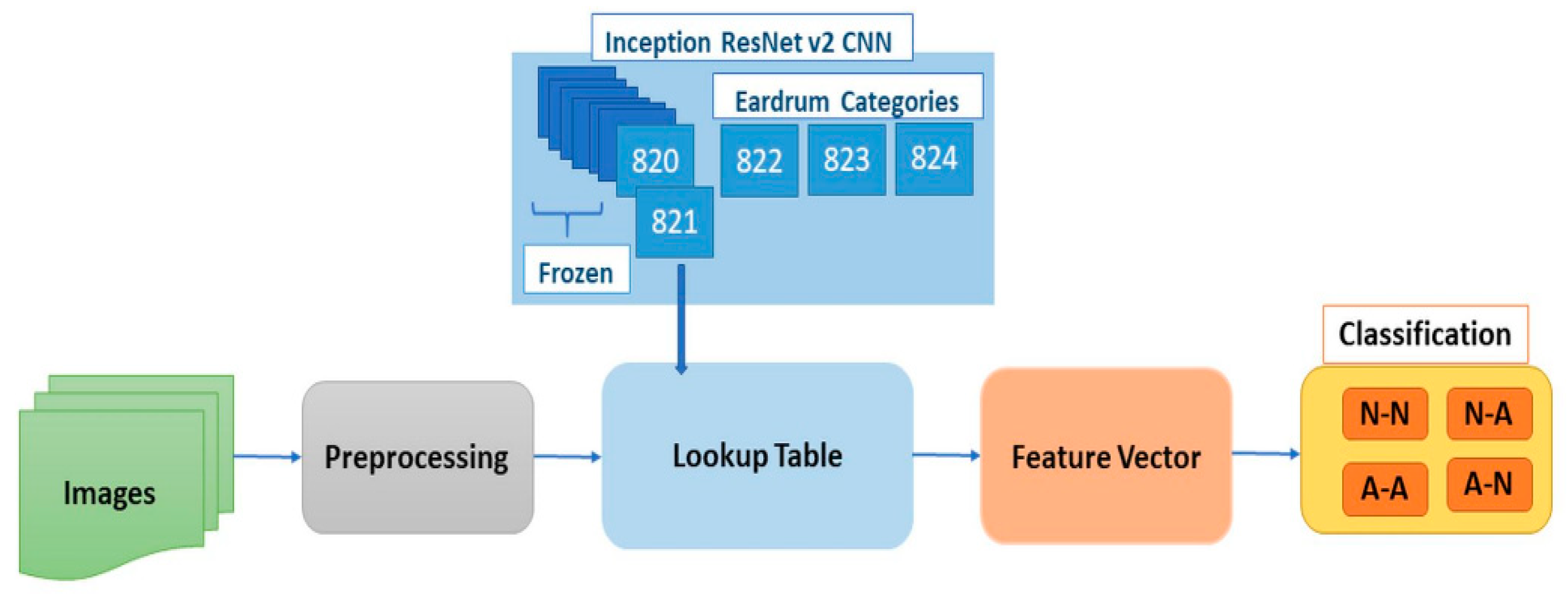
Our pairwise classification system, OtoPair, has the following components: preprocessing and data augmentation, feature extraction to generate a lookup table, feature vector formation for a pair of eardrum images, and normal/abnormal classification for the pairs (see
Figure 1).
The pre-processing steps remove the black margin and date/time text on the images, as explained in our previous study, OtoMatch [
19]. The feature extraction is completed in two steps: transfer learning-based and handcrafted. In order to obtain transfer learning-based lookup table features, we used the infrastructure of our previous work [
19]. Finally, the paired images were classified, and the performance of the system was evaluated by 10-fold validation.
2.1. Dataset
All of the images used in this study are captured from adult (174 ears) and pediatric (124 ears) patients at primary care clinics and Ear, Nose, and Throat (ENT) facilities of the Ohio State University (OSU) and Nationwide Children’s Hospital (NCH) in Columbus, Ohio, US with the IRB approval (Study Number: 2016H0011). The images from adult patients were collected in clinic by a board-certified ENT physician with fellowship training in neurotology (i.e., a clinical focus on ear disease); images from pediatric patients were collected in the operating room at the time of tympanostomy tube placement by a board-certified ENT physician with fellowship training in pediatric otolaryngology. Additionally, conforming to the rules set by the Ohio State University Institutional Review Board, all of the samples were fully anonymized while creating the experimental dataset.
In this study, a total of 150-pair (i.e., 300 individual) eardrum images were used to train and test the system, with images being included if a complete image pair was available (i.e., images from both ears were available and had sufficient focus and lighting to evaluate the eardrum), and were diagnosed as normal, middle ear effusion, or tympanostomy tube present. Each pair consists of the right and left ear images of the same person that were captured in the same visit.
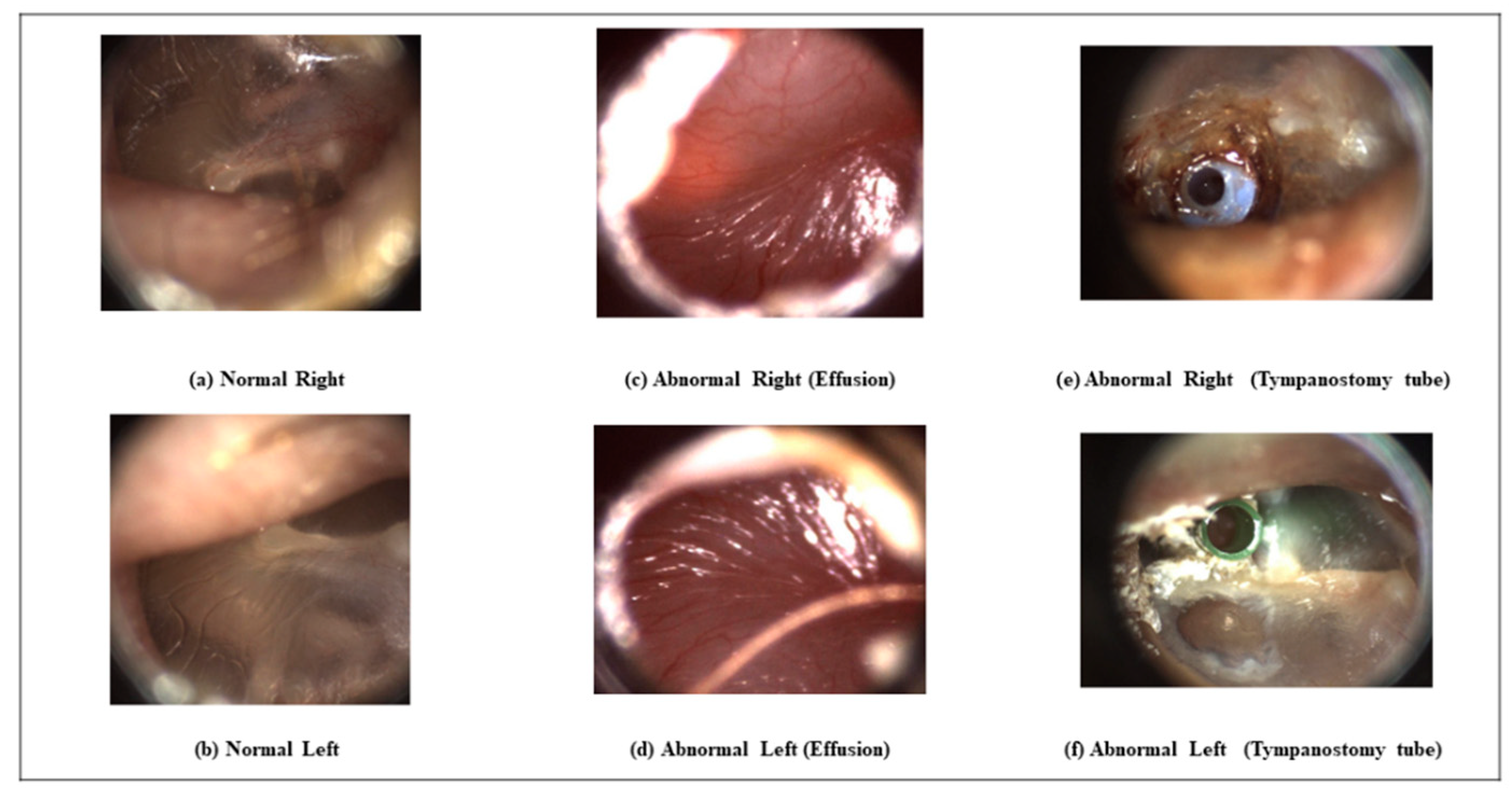
Table 1 shows the number of images for each category (normal-abnormal). We only included two categories of abnormality: effusion (fluid) of the middle ear and tympanostomy tube because there was not a sufficient number of images in other categories to train and test our classifiers properly. Again, for the same reason, we investigated the problem of normal-abnormal pair classification, as opposed to classifying the pairs according to the type of abnormality separately. In addition to the number of pair images, 137 single images (83-Abnormal, 54-Normal) were used to validate the developed system’s deep learning part while extracting the lookup table features.
Figure 2 shows paired examples from normal, abnormal with effusion, and abnormal with tympanostomy tube categories, demonstrating the variability among the images in different categories. The images from some categories are difficult to distinguish from the others for an untrained person. In many cases, the similarities between the right and left ear are not obvious. The tympanostomy tube abnormality appears differently for the same patient, as can be seen in
Figure 2e,f.
We used all of the paired image datasets because increasing the number of paired images was critical in this study. The database contained images that were captured in the JPEG format. Additionally, we selected individual images from the frames of otoscopy video clips. Both single images and video frames were the same size (1440 by 1080 pixels) and resolution. Some of the images in the video frames were unfocused, contained large amounts of wax, or did not have the proper illumination. Therefore, we manually selected the best single images and frames to form the appropriate pair of images.
2.2. Data Augmentation and Preprocessing
A data augmentation approach was used to increase the number and diversity of images for transfer learning. The augmentation approached included reflecting images both horizontally and vertically, scaling images in the range of 0.7 to 2, randomly rotating images, shearing images both horizontally and vertically within a range of 0 to 45 degrees, and then translating them within a pixel range from −30 to 30 pixels in both the horizontal and vertical directions.
Regions of interest (RoI) were extracted in the preprocessing step, which is the same as our previous study OtoMatch, in order to extract features from these images [
19]. The preprocessing step included reducing the black margin and embedded text (to mark the capture date and time), which may negatively affect the features.
2.3. Forming Feature Vector
In order to classify the eardrum pairs as normal or abnormal, the feature extraction was completed in two steps: transfer learning-based lookup table feature extraction and handcrafted feature extraction. The transfer learning-based lookup table features are the same as in our previous work [
19] for the eardrum image retrieval system. In this study, they were integrated into the pairwise classification system (
Section 2.4). The handcrafted features included registration error, histogram, and statistical measurements of the a* and b* components of the L*a*b* color space.
2.3.1. Transfer Learning based Feature Extraction
In our previous work [
19], Inception-ResNet-V2 Convolutional Neural Network (CNN) was used. It was pre-trained and validated with 50,000 images set to classify 1000 object categories and learned rich feature representations with 825 layers. A huge number of images is required to re-train the whole network. The first 820 layers were frozen to limit the number of parameters required to retrain the network to avoid overfitting with our limited dataset. The last three layers (prediction, softmax, and classification) of the pre-trained network were retrained with otoscope images in our database.
After retraining the network, the resulting features were subjected to pooling that mapped each image into a vector of 1536 features. We relied on the fully connected layer’s output, which produced vectors for each training and test image, where three represents the number of image categories in our database: normal, effusion, and tympanostomy tube. The features formed a vector at the output of the average pooling layer. Therefore, the weights were a matrix of the fully connected layer. When the transpose of the feature vector was multiplied by the weight vector, it produced a vector, which was established for each of the training set of images. When these vectors were turned to rows of a matrix (), this constitutes the lookup table.
This procedure was applied to a pair of eardrum images for normal/abnormal feature extraction. Inception-ResNet-V2 pre-trained CNN was used by freezing the first 820 layers. In this study, the number of categories was two (i.e., normal, abnormal), and the weights constitute a matrix of the fully connected layer. The generated lookup table is a vector of length where is the number of training images. Additionally, test images have a vector after multiplying them by weights. For each pair of the eardrum images, these lookup values are calculated, and a new feature vector is formed using these values.
The steps to create a lookup table from transfer learning can be generalized, as follows:
Form a feature vector as the average pooling layer output for each image, . Its size is (F = 1536 in this case).
Let of size be the weights of the fully connected layer, where C is the number of training classes ( in this case because of two categories: ‘normal’ and ‘abnormal’).
The lookup table values for one image, , can be calculated as , and its size is .
If is the number of images in the dataset (both for training and testing), the lookup table is a matrix calculated as concatenation of the lookup table values for each image, and with a size ( for this case).
The lookup table values of the right eardrum image are R1 and R2, and of the left eardrum image are L1 and L2. Their ratio (R1/L1, R2/L2), summation (R1 + L1, R2 + L2), and difference (R1 − L1, R2 − L2) are also concatenated to form a feature vector. This new vector, which contains both eardrum pairs’ features, enables us to classify the pair together by combining the derivative of lookup table values for a pair of eardrum images.
2.3.2. Handcrafted Feature Extraction
In addition to the lookup table-based features, we also used handcrafted features, which captured the registration errors between the pair eardrum images. The registration is used to match and compare two or more images that were obtained at different times from different sensors or different viewpoints to find the best transformation that portrays good spatial correspondence among them [
24,
25]. Image registration is frequently used in medicine to align images from different medical modalities for diagnosis, treatment monitoring, surgery simulation, radiation therapy, assisted/guided surgery, and image subtraction for contrast-enhanced images [
26,
27,
28,
29]. In our study, we used image registration to calculate the error between the pair of eardrum images and use it as a feature to classify pairs together.
Eardrum image registration is challenging, even for normal cases, because the malleus is positioned differently in the eardrum images of the right and left sides of the same person. Furthermore, the pair images are rarely symmetric, nor are they obtained from the same perspective when captured with an otoscope. For diseased eardrums, registration is more challenging than that for normal cases, because some diseases (e.g., effusion) lead to changes in the eardrum shape and cannot be easily detected with 2D images.
We used both rigid and non-rigid registration. For both types of registration, there should be moving and target images; moving (source) images transform spatially to align with the target (fixed, sensed) image. Rigid registration [
30] includes the translation, scaling, and rotation of the moving image to the target image, and non-rigid matching is done using the demons method [
31], which transforms the points, depending on Maxwell’s demons and matches the deformed parts of the image. The basis of demon registration forces finds small deformations in temporal image sequences by calculating the optical flow equations. Therefore, the Thirion method estimates the displacement [
31] for corresponding match points. Gaussian smoothing is used for displacement for regularization because the demons equation approximates the local displacement in each iteration.
Before registration, each image is converted from color (RGB) to a gray-scale image, and the registration is applied to the gray-scale images. For rigid registration, mutual information is used as the similarity metric. For optimization, a one-plus-one evolutionary optimization algorithm [
32,
33], which iterates the set of parameters to produce the best possible registration, is used with the initial radius’s parameter is 0.009, epsilon is 1.5 × 10
−4, the growing factor is 1.01, and a maximum of 300 iterations. After rigid registration, non-rigid demon algorithm image registration [
34] with a single modality parameter is applied to a rigid registered image.
The mean square error between the fixed image and registration images is computed as the difference of corresponding pixels and taking the mean square of them and used as a similarity metric between the fixed and moving images. One of the mean square errors is computed after rigid registration, and another one is after non-rigid registration. These two mean square errors concatenated to feature vector starts with lookup table based values.
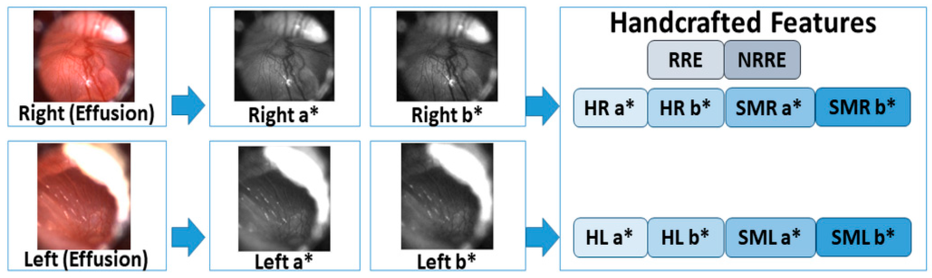
Lastly, we used a* and b* components of the L*a*b* color space of each pair of eardrum images to extract color-based features to accurately classify the pairs. The L*a*b* color space is the uniform color space with equal distances on the x, y chromaticity diagram corresponds to equal perceived color difference. In this color space, L* indicates lightness, and a*and b* are the chromaticity coordinates, where +a* is the red direction, −a* is the green direction, +b* is the yellow direction, and −b* is the blue direction. The RGB color images are converted to the L*a*b* color space, and the histogram and statistical measurements of the a* and b* bands are calculated. The histogram of color bands is divided into ten bins, and the number of each bin is concatenated to the feature vector for each pair of images. There are 40 histogram values, which come from two images (right and left images) and two bands (a* and b* bands) for each ear pair. In addition to the histogram values, statistical measurements of mean, standard deviation, skewness, and kurtosis of each band of pairs. A total of 16 features come from these four statistical measurements.
Figure 3 shows a graphical summary of the new feature vector formation.
2.4. Classification
After the feature vector of the pair (right and left) eardrum images was formed by concatenating the lookup table values with handcrafted features, these are classified. In order to classify a pair of images together, we aimed to collect all of the features in one vector for each pair. Thus, we could analyze the difference between classifying single images and classifying pairs as ‘Normal-Normal’ (N-N), ‘Abnormal-Abnormal’ (A-A), ‘Normal-Abnormal’ (N-A), and ‘Abnormal-Normal’ (A-N). Single image classification results were obtained after retraining the Inception ResNet-v2 pre-trained network by changing the last three layers according to ‘Normal/Abnormal’ classes of eardrum images and frozen the first 820 layers to avoid an overfitting of the network. The number of frozen layers was empirically determined from our previous study OtoMatch as 820. For the paired image classification, a newly created feature vector is used in the Tree Bagger algorithm.
The Tree Bagger algorithm is the ensemble model of bootstrap aggregated decision trees. Multiple decision trees constitute resampling training data with replacement again and again, and voting the trees for majority prediction [
35]. These decision trees are the classification trees whose leaves represent class labels; branches represent conjunctions of features that convey to these class labels. In our problem, the leaves are the ‘Normal’ and ‘Abnormal’ class labels, and the branches are the conjunction of the feature vector. The out-of-bag (OOB) error method [
36] was utilized to measure the prediction error of boosted decision trees models to sub-sample data to train the method. The OOB error is measured by excluding a sub-sample from the training data and calculating the mean prediction error in the bootstrap sample [
37]. Subsampling improves the prediction performance by evaluating predictions on observations that are not used in building the tree (defined out-of-bag).
This study modeled the decision tree using the TreeBagger supervised machine learning function in Matlab 2019b software. Selected trees, where the observation is out of the bag, compose the class posterior probabilities’ weighted mean. Accordingly, the predicted class is the largest weighted mean of a corresponding class. This is also designed to improve the model’s stability and accuracy by reducing the variance without raising the bias. The optimal number of trees decided according to the out-of-bag error changes with the accumulation of trees. In our study, the number of classes (normal and abnormal) and the number of observations (150 pair eardrum image) limit the number of decision trees, which is empirically selected to be five.
2.5. Experimental Setup
We selected 150-pair images (see
Table 1) from normal and abnormal (effusion and tympanostomy tube) categories, which have the highest number of paired images in our database. Even after we enhanced our database with selected video frames of the videos, our dataset contained 150 paired eardrum images to train the model. Even though we know that the balanced amount of data for each category would avoid the bias towards the majority classes and minimize the overall error rate, we could not add more normal-abnormal pair images to our dataset because of the limited number of cases.
Our limited number of pair images was used for both training and testing groups of data. Our system had two training steps: one for the transfer learning training and the other for the random forest classifier training. We used a separate validation dataset for transfer learning training, which contained single 83 ‘normal’ and 54 ‘abnormal’ eardrum images (not pairs) during the retraining of the lookup table generation feature extraction phase. We could allocate more cases for training because we used a separate dataset for validation.
We used k-fold (k = 3) cross-validation to test the generalizability of our results. Because the number of ‘normal-abnormal’ and ‘abnormal-normal’ pair images was low, the fold number (k) was also kept low. The paired images were divided into three random groups for each category: one group was used for testing and the other two groups were used for training. The training group was used to learn the network parameters in transfer learning and fit a model for the tree bagger classifier part. Because the data were divided into groups before the system was run, we put the same pair in the same group, either in training or testing. Accordingly, we made sure that each patient’s eardrum image pairs were used for either training or testing, but not both.
The tree bagger algorithm was also evaluated with a three-fold cross-validation method. To properly model the system, the size of the dataset and number of categories play an important role in the tree bagger classifier. We empirically decided to use five trees to model the classifier because we had 100 pairs for training and 50 pairs for testing and the number of categories was four (N-N, N-A, A-A, A-N).
3. Results and Discussion
We used single eardrum images to train and test the system for the transfer learning part of the training with classification accuracy as a measure for each training fold. We retrained the transfer learning for extracting the lookup table values twice: before and after adding normal-abnormal image pairs. Because the number of ‘normal-abnormal’ pair images was limited, we started with ‘normal-normal’ and ‘abnormal-abnormal’ pair images and with the classification categories of normal or abnormal. Subsequently, we performed the experiments adding ‘normal-abnormal’ eardrum pair images and compared them.
Table 2 shows these two experimental results for these cases.
Before adding normal-abnormal pairs’ eardrum images, training, validation, and testing accuracies were 88.8% ± 3.3%, 86.7% ± 6.7%, and 83.3% ± 3.3%, respectively, as seen in
Table 2. However, adding normal-abnormal cases decreased the accuracies for to 83.6% ± 6.3%, 78.4% ± 6.8%, and 78.7 ± 0.1%. This training step was used just for creating a lookup table and extracting lookup table features.
After creating the lookup table with transfer learning, we experimentally tested the lookup table-based feature extraction and handcrafted feature extraction (see Methodology Section). Lookup table based feature extraction was the first step of the feature extraction phase. The handcrafted features were registration errors, the number of counts in bins of the histogram of L*a*b*, mean, and other statistical measurements (standard deviation, skewness, and kurtosis), and these were concatenated in each step, and the system was tested after each concatenation.
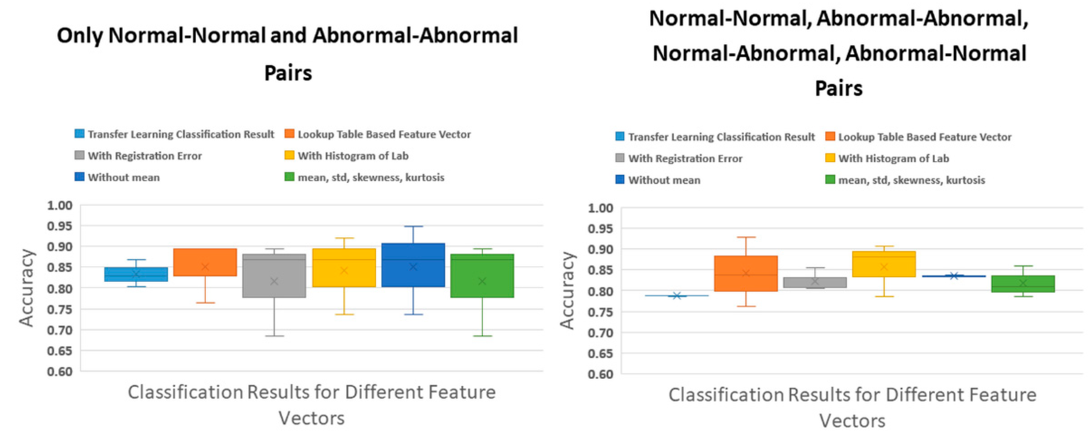
Figure 4 presents the system accuracies for normal-normal (N-N), abnormal-abnormal (A-A), and all pairs (N-N, A-A, N-A, and A-N). After adding N-A, A-N pair images, the accuracies decreased. Before the N-A pairs added to the dataset, the lookup table based feature extraction accuracy result was the highest accuracy with 85.1% and 7.6% low standard deviation. After adding A-N pairs, the highest accuracy result was 85.8% ± 6.4% for concatenated registration error and histogram of L*a*b* features to the lookup table based features.
When the paired image classification accuracies are compared with those of the single images, we observe some improvements from 83.3% (SD ± 3.3%) to 85.1% (SD ± 7.6%) (N-N and A-A pairs) and from 78.8% (SD ± 0.1%) to 85.8 (SD ± 6.4%) (N-N, A-A, N-A, and A-N pairs). Unfortunately, most of the improvements are not statistically significant according to the t-test between the classification results of transfer learning and each tested pair features. For the same category pair (i.e., N-N and A-A) images, the average p-value is 0.80, while, for all category pair (N-N, A-A, N-A, and A-N) images, the average p-value is 0.16. While the p-values decreased, they were not statistically significant (<0.05). However, the p-value of the t-test between the classification results of transfer learning and all features (except for the mean value of the L*a*b* color space) is 0.0004, which is statistically significant. The reason is standard deviations of both results for three-fold cross-validation are 0.1%, and 0.2%, while their accuracy values are 78.7% and 83.3%, respectively. Hence, all three-fold results were consistent with just small differences.
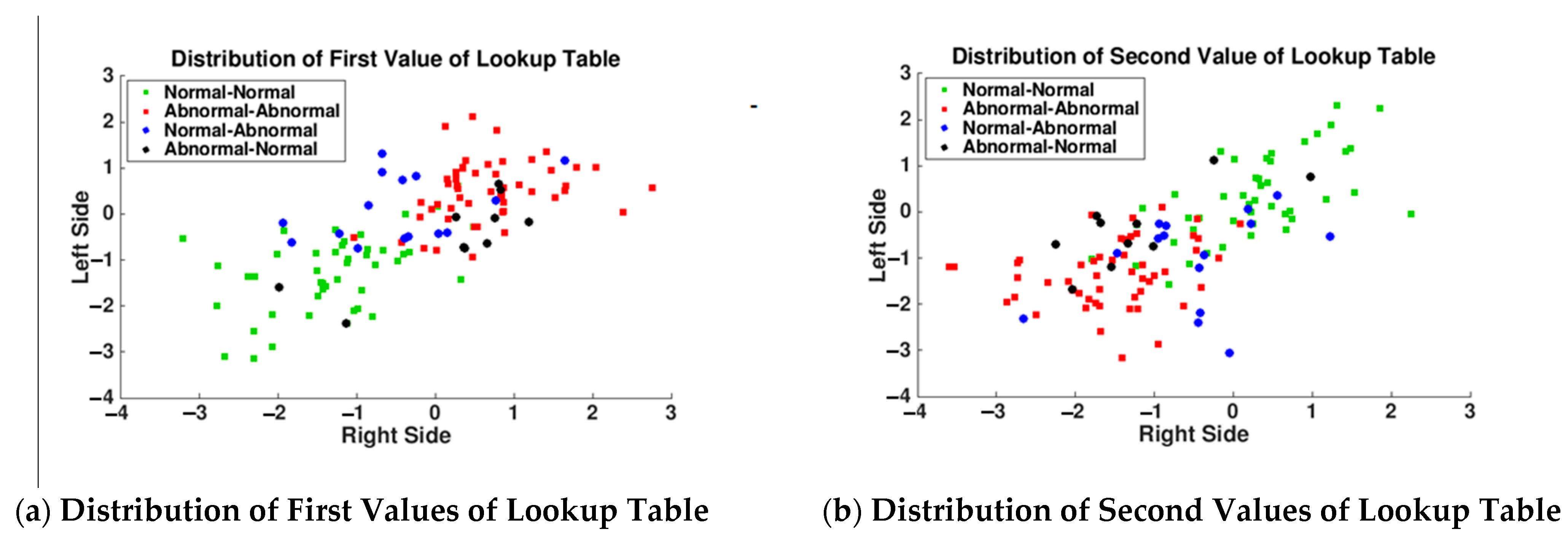
In
Figure 5, because N-N and A-A pair distributions were well separated into separate quadrants of the feature space, our expectation was the normal-abnormal pair values distributed to the other quadrants. For example, in
Figure 5a, N-N pairs both right and left values less than 0, A-A pairs values greater than −0.5, and A-N (ear pair right side abnormal and left side normal) pairs (represented with a black circle) supposed to distribute lower-right quadrant of the figure. Likewise, for N-A (ear pair right side normal and left side abnormal) pairs (represented with blue circle) are supposed to distribute the upper-left quadrant of
Figure 5a. However, black and blue circles mixed in N-N and A-A pair values are presented in
Figure 5a,b. This caused a decrease in the accuracies for transfer learning test results and lookup table based feature extraction system results after adding normal-abnormal pair images.
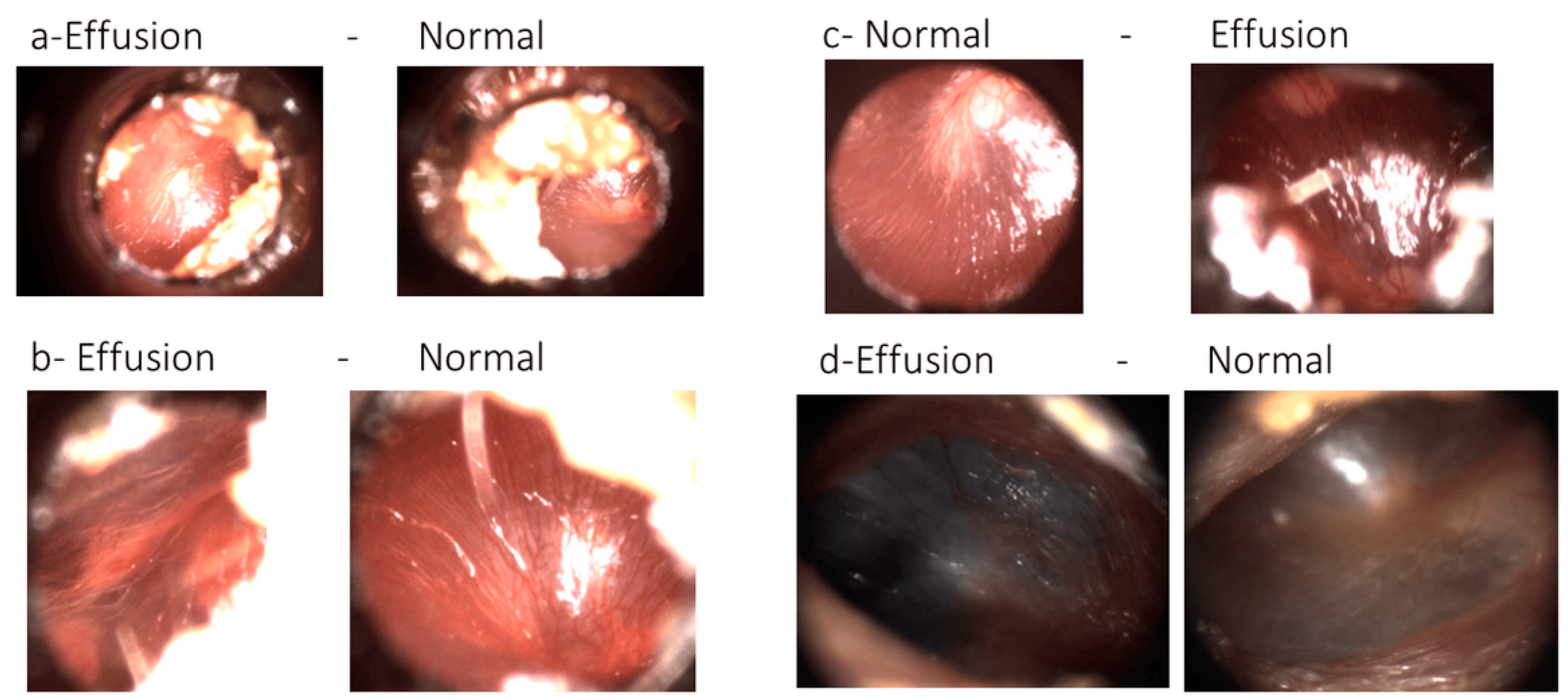
After we observed these unexpected distributions of blue (i.e., N-A) and black circles (i.e., A-N), our ENT expert examined the normal-abnormal pair images, which were selected from video frames of both adult and pediatric patients’ otoscope video clip. He labeled the normal-abnormal pair images as ‘subtle’ or ‘not subtle’, and 63.3% (19/30) of the pair images were labeled as ‘subtle’.
Figure 6 illustrates four examples of pair images that were labeled as ‘subtle’ by our ENT specialist and misclassified by transfer learning.
Imaging problems may be the reason for misclassification. Three pairs had illumination problems that manifest themselves on images as yellow or white light spots, which makes it difficult for the camera to focus on the eardrum region. Another common problem was ear wax and hairs, because they were closer than the eardrum to the otoscope, reflecting light. Furthermore, the eardrum region of the image was not enough to classify its category. The blurry parts of the images were another problem with these images. The second column of
Figure 6 demonstrates images with out of focus problems. While
Figure 6c-Normal is an in-focus image,
Figure 6c-Effusion is blurry between the two regions with light reflections. In contrast,
Figure 6d-Effusion and d-Normal contain blurry regions, regardless of the amount of light reflection.
The accuracy of the system will likely decrease, depending on the problems (light, wax, hair, or blurring) of the normal-abnormal pairs’ images. However, it should be noted that some of these problems (e.g., obstruction of the view by wax) also remain current barriers to traditional clinical otoscopy. Nonetheless, for this study, we wanted to experimentally test and investigate the normal-abnormal cases with a limited amount of data. While the improvements in accuracies are not statistically significant (most likely because of limited data), we still observed an increase in them using our approach, and this increase could likely be due to additional features that are extracted from the paired images and used together. Our paired image classification approach is the first for classifying pair eardrum images together, and the results are promising.
OtoPair is a novel system that classifies a pair of eardrum images together, which takes advantage of the similarities between the eardrums of an individual. This approach builds upon our previous OtoMatch content-based image retrieval (CBIR) system by creating deep learning-based lookup tables. Thus, OtoMatch sets up the infrastructure for the OtoPair system to find the similarities between a pair of eardrums. OtoPair extracts additional features, such as those that are derived from color and registration error, to classify the pair images. Additionally, OtoMatch is a content-based eardrum image retrieval system, not a classifier. OtoMatch was trained for normal, middle ear effusion, and tympanostomy tube conditions, while OtoPair was trained for ‘normal’ and ‘abnormal’ eardrum images.
4. Conclusions
In this study, we propose a system for classifying pair eardrum images together as ‘normal-normal’, ‘abnormal-abnormal’, ‘normal-abnormal’, and ‘abnormal-normal’. To the best of our knowledge, this is the first study that classifies a pair of eardrum images of the same patient together. We used two feature extraction methods to classify the pair of images: deep learning-based and handcrafted, and combined the resulting features of two sides of eardrum images to classify the pair of images together. Subsequently, we analyzed the results of one side of eardrum images and pair eardrum images with and without ‘normal-abnormal’ and ‘abnormal-normal’ cases.
We also compared the results after extracting each group of features of the paired images. According to the experimental results, the highest accuracy was 85.8% (±6.4%) for all types of pair image classification. The features of concatenated registration error and histogram of L*a*b* features. However, the only statistically significant result of the difference between single side eardrum image classification with transfer learning was due to all of the extracted and concatenated features (without the feature of the mean of L*a*b* color space) with 83.5% (±0.2%) accuracy. Other experiments did not create any statistically significant difference. Still, at least one statistically significant result is promising with all concatenated features, except the mean of L*a*b* color space features.
One of the study’s limitations is the small number of A-N (abnormal-normal) paired images, and the abnormal class only consists of otitis media effusion and tympanostomy tube categories. In addition to this, 63.3% (19/30) of the existing A-N pair images were subtle as assessed by a specialist. Future studies will include a larger number of pair images for each category of eardrum pairs. We also observed that transfer learning based lookup table values for the same category pairs could be easily classified according to differently labeled pair images. Therefore, we can use the lookup table values to select subtle images and automatically eliminate them from the training dataset for future studies.


 ,
, 


