Abstract
Since 2009, China has implemented two important place-based policies to promote e-commerce development in selected cities: “Building National E-commerce Demonstration Cities” and “Comprehensive Pilot Zones for Cross-Border E-commerce”. Previous studies reported that these two e-commerce development policies generated local environmental benefits by reducing air pollution and carbon emissions in the policy implementation areas. However, whether these policies have spatial spillover effects on environmental quality in other regions and the extent of such effects have not been sufficiently analyzed. This study aims to empirically assess the environmental spatial spillover effects of these two policies. Based on panel data from 221 prefecture-level cities in China from 2000 to 2021, this study utilizes a spatial econometric regression method to evaluate the policy effects. The study yields three main findings. (1) The policies significantly reduced air pollution concentrations and carbon emissions while increasing vegetation greenness in non-policy implementation areas. Specifically, the policies led to reductions in carbon monoxide (CO), nitrogen dioxide (NO2), fine particulate matter (PM2.5), sulfur dioxide (SO2), and the emissions of carbon dioxide (CO2), as well as increases in the fractional vegetation cover (FVC), normalized difference vegetation index (NDVI), and net primary productivity (NPP). Our findings indicate that the environmental effects of e-commerce development policies extend beyond the policy-implementing areas. (2) Further heterogeneity tests reveal that the beneficial spatial spillover impacts of e-commerce development policies were observed in cities with different geographical locations, servicification levels, economic scale, and population densities. (3) Mechanism analysis shows that although the policies did not alter the environmental regulation stringency in non-policy regions, they promoted industrial structure upgrading, technological advancement, and green innovation in these areas, thereby explaining the detected spatial spillover effects.
1. Introduction
1.1. Research Background
Globally, the rapid expansion of e-commerce has profoundly reshaped business landscapes and consumption patterns. As the world’s largest online retail market, China has drawn particular attention for its swiftly growing e-commerce penetration and continuous business model innovation [1,2]. While this trend fuels economic growth and enhances social convenience, it has also sparked widespread concern over its environmental externalities. E-commerce inherently carries the potential for environmental benefits—such as improved resource efficiency and reduced carbon emissions—through intensification and digitalization. Yet, its development is also accompanied by environmental challenges, including packaging waste and rising energy demands. Therefore, a comprehensive assessment of the net environmental influence of e-commerce is crucial and serves as a foundational step toward fostering sustainable development of e-commerce.
Some previous studies have conducted ex-post evaluations on the environmental effects of e-commerce development. Likely due to the higher data availability on air pollution and carbon emissions, these studies have focused on air pollution and carbon emissions. Most of the literature found that e-commerce development helps reduce local air pollution and carbon emissions.
It is noteworthy that the environmental consequences of e-commerce are likely not confined locally; rather, they may exert significant spatial spillover effects on other regions through channels such as technology diffusion, logistics networks, energy consumption, and industrial relocation. However, so far, the existing literature has paid insufficient attention to this specific research area.
1.2. E-Commerce Policy Context in China
To encourage and promote the development of e-commerce, the Chinese central government has implemented two important place-based e-commerce development policies in recent years: the “Building National E-commerce Demonstration Cities” (BNEDC) policy and the “Comprehensive Pilot Zones for Cross-Border E-commerce” (CPZCE) policy. These two policies are implemented only in a set of specific regions selected by the central government, while other cities are not covered [3,4]. In the covered areas, the central and local governments invest resources (such as funding, tax incentives, institutional support, and infrastructure investment) to encourage and support businesses in developing e-commerce operations. The governments aim to foster local economic prosperity through the growth of e-commerce and to provide valuable lessons for cities not included in the policies [5,6]. The two policies are generally similar in content. Beyond differences in geographical coverage and launch dates, their key distinction lies in their focus: whereas the BNEDC aims to promote e-commerce development in a broader sense, the CPZCE places a stronger emphasis on cross-border e-commerce and international trade.
In 2009, Shenzhen City in Guangdong Province was selected as the first city to implement the BNEDC policy [7]. In 2015, Hangzhou City in Zhejiang Province became the first city to implement the CPZCE policy [8]. Subsequently, an increasing number of cities have been included under these policies. Figure 1 shows the number of cities implementing these two e-commerce development policies between 2005 and 2023. As demonstrated in the figure, the number of cities covered by the BNEDC policy stopped increasing after 2016, while the number of cities covered by the CPZCE policy continued to rise. Since many cities that implemented the BNEDC policy in earlier years later adopted the CPZCE policy, there is a substantial overlap in the coverage of the two policies. By 2023, most cities under the BNEDC policy had been incorporated into the CPZCE policy coverage.
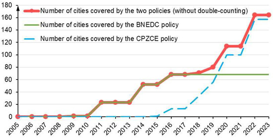
Figure 1.
The number of cities implementing two e-commerce development policies during 2005–2023. Data source: The lists of policy implementation cities in different years were published by the Chinese central government. When counting the number of cities, we considered prefecture-level cities and provincial-level municipalities, but did not include the few county-level administrative districts mentioned in the policy document.
In this study, we regard the BNEDC and CPZCE policies as two components of one policy category. In the empirical analysis of this paper, we refer to these two policies collectively as the “e-commerce development policy”. The rationale for this approach is explained as follows. (1) The content of these two policies is largely similar, primarily encompassing the following aspects: promoting the development and application of new information technologies; improving the institutional environment and reducing transaction costs; encouraging the development of new business models and industrial upgrading; fostering economic growth and employment; and advancing the green economy. After 2016, the number of cities covered by the BNEDC policy ceased to expand, while the CPZCE policy was implemented starting in 2015. Therefore, it is reasonable to consider the CPZCE policy as a continuation and extension of the BNEDC policy. (2) There is a high degree of overlap between the cities covered by these two policies. Particularly before 2018, almost all cities covered by the CPZCE policy had previously been covered by the BNEDC policy. Most cities that implemented the BNEDC policy later adopted the CPZCE policy as well. The significant overlap between the two policies makes it difficult to strictly distinguish their respective impacts.
The implementation of BNEDC and CPZCE policies has effectively promoted the expansion of China’s e-commerce and the prosperity of related industries [9,10,11]. Figure 2 illustrates the growth of China’s countrywide e-commerce sales from 2005 to 2023, as well as the increase in the number of cities implementing the two e-commerce development policies. As the number of policy-implementing cities continued to rise, the national e-commerce scale expanded rapidly, growing from less than 1 trillion CNY (approximately 0.1 trillion USD) in 2005 to over 50 trillion CNY (approximately 7.1 trillion USD) in 2023.
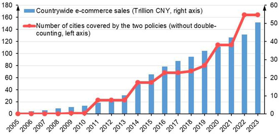
Figure 2.
Growth of China’s countrywide e-commerce sales and the number of cities implementing two e-commerce development policies during 2005–2023. Data source: The data on e-commerce sales was sourced from the website of the Ministry of Commerce of China. The lists of policy implementation cities in different years were published by the Chinese central government. When counting the number of cities, we considered prefecture-level cities and provincial-level municipalities, but did not include the few county-level administrative districts mentioned in the policy document.
Admittedly, correlation is not equivalent to causation, so Figure 2 alone cannot demonstrate that e-commerce development policies significantly contributed to the expansion of the e-commerce scale. To further illustrate the outcomes of these policies, we present Figure 3. This figure uses a binned scatter plot (controlling for province- and year- fixed effects) to show the positive correlation between the provincial share of cities with e-commerce policies (as a share of the national total) and the provincial share of e-commerce sales (as a share of the national total) during the period 2012–2021. If e-commerce development policies indeed effectively promoted the expansion of local e-commerce scale, we should observe that e-commerce activities were heavily concentrated in policy-covered cities. Therefore, provinces with a higher share of policy-covered cities relative to the national total should also exhibit a larger relative scale of e-commerce. This is exactly what Figure 3 demonstrates.
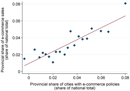
Figure 3.
The positive correlation between the provincial share of cities with e-commerce policies (share of national total) and the provincial share of e-commerce sales (share of national total) during 2012–2021. Note: (1) The authors calculated the statistics and drew the figure based on provincial e-commerce sales data from the CNRDS database and the list of policy implementation cities published by the Chinese central government. (2) When creating this figure, we only used data from 2012 to 2021, as provincial-level e-commerce sales data for other years were unavailable. (3) The province- and year-fixed effects are excluded. (4) The binned scatter plot is drawn by using 20 bins. The figure is similar if alternative bin numbers are selected.
In brief, China’s implementation of e-commerce development policies has provided a valuable natural experiment, allowing researchers to employ policy evaluation methods to explore the consequences of e-commerce expansion.
1.3. Research Objective and Contributions
The objective of this study is to examine whether China’s e-commerce development policies have generated spatial spillover effects on the environment. To this end, we collected the annual-frequency panel data from 221 prefecture-level cities in China between 2000 and 2021 and employed a spatial econometric regression approach to estimate the policy impacts.
This research makes research contributions in the following two aspects.
- (1)
- Existing studies have not sufficiently analyzed whether the development of e-commerce has a spatial spillover influence on environmental quality. Our research fills this gap by empirically demonstrating that China’s two important e-commerce development policies can significantly benefit environmental quality in non-policy implementation areas. This finding contributes to a deeper understanding of the environmental implications of e-commerce. Our study reveals the existence of spatial spillover effects in e-commerce development, indicating that some conclusions and policy evaluations in the previous literature that did not account for such spillover effects may be biased. Our research also highlights the need for policymakers to explicitly consider spatial spillover effects and policy externalities when designing e-commerce development strategies, and to coordinate policies across regions. Only through appropriate policy design and coordination can the overall impact of regional policies be optimized.
- (2)
- This paper examines multiple environmental quality indicators, including concentrations of various air pollutants, carbon emission scale, as well as vegetation greenness levels. Compared to previous related studies, our analysis provides a more comprehensive portrayal of the multidimensional changes in environmental quality in China. The analysis offers new empirical evidence for understanding the country’s environmental issues. Our findings demonstrate that e-commerce development policies can influence a wide range of environmental indicators. This suggests to both researchers and policymakers that the environmental impacts of e-commerce are multidimensional, extending beyond the narrow set of indicators—particularly PM2.5 and carbon emissions—that have been the primary focus of existing literature.
The remainder of this paper is structured as follows. Section 2 reviews the relevant literature and develops the research hypotheses. Section 3 explains the empirical model, variables, data sources, and the study sample. Section 4 presents a series of empirical results, including the core findings, robustness checks, heterogeneity tests, and mechanism analyses. Section 5 discusses the academic and practical implications of the study. Finally, Section 6 concludes the paper and outlines the research limitations as well as potential directions for future research.
2. Literature Review and Hypothesis Development
2.1. Literature Review
This study is closely related to two strands of literature. The first strand involves assessing the environmental impacts of e-commerce development. The second strand focuses on evaluating the outcomes of China’s BNEDC and CPZCE policies.
2.1.1. Environmental Impacts of E-Commerce
Ex-post assessments of the environmental impacts of e-commerce development have been undertaken in some prior studies. These studies have predominantly concentrated on air pollution and carbon emissions, likely due to the greater data availability for these metrics. A consensus emerging from this stream of empirical literature indicates that e-commerce development generally plays a role in mitigating local atmospheric pollution and carbon emissions. For instance, Manta et al. [12] and Xie et al. [13] reported empirical evidence from European countries on carbon emissions; Liu et al. [14] provided evidence from China on carbon emissions; Chen and Yan [15] and Yu et al. [16] reported evidence from China on air pollution.
While the local environmental impacts of e-commerce have been studied, it is also crucial to consider its potential spatial spillover effects. These policy effects are likely transmitted to other regions through channels such as technology diffusion, logistics networks, energy consumption, industrial relocation, and even the structural transformation of the overall economy. These spillover effects act as a double-edged sword. On the one hand, the development of e-commerce may generate beneficial environmental spillovers: by optimizing supply chains and reducing individual travel [17,18], it lowers energy consumption and pollution emissions in other regions; simultaneously, the new technologies fostered and applied through e-commerce may also benefit other areas via technology diffusion [19], enhancing their ecological efficiency. On the other hand, e-commerce could lead to harmful environmental spillovers: for instance, the surge in packaging waste and decentralized transportation may increase pollution emissions in other regions [20,21]; additionally, changes in industrial structure driven by local e-commerce development might result in the relocation of polluting industries to neighboring areas [22]. Therefore, to discern the net effect and underlying mechanisms of e-commerce on the environment in other regions, it is necessary to conduct quantitative evaluation using empirical data. The existing literature has yet to adequately address this area of research.
2.1.2. Impacts of China’s E-Commerce Development Policies
China’s e-commerce development policies create a valuable natural experiment. Researchers can leverage this context to employ policy evaluation methods, thereby effectively exploring the outcomes of e-commerce growth. Existing literature includes several studies that utilized the difference-in-differences (DID) method—a classic policy evaluation approach—to assess the impact of China’s BNEDC and CPZCE policies on the local environment in policy-implementing areas. The findings of these studies are consistent, indicating that both policies reduced local air pollution [23,24,25] and carbon emissions [26,27,28,29]. However, these existing studies share a notable limitation. A key assumption of the DID method is the absence of spatial spillover effects, which is called the “stable unit treatment value assumption” (SUTVA) [30,31]. If spatial spillover influences exist, the results of DID analysis would be substantially biased, potentially leading to either underestimation or overestimation of the impacts of policies. In this case, the results of the policy evaluation would provide policymakers with inaccurate or even misleading reference information. Therefore, investigating whether China’s e-commerce development policies generate environmental spatial spillover effects is of great practical significance.
Prior studies on various countries have indicated that trade or economic policies implemented by governments in one region or country may generate spillover effects on the environment of other regions. For instance, Santika et al. [32] examined 195 countries worldwide and found that regional trade agreements amplify environmental impact shifting, particularly in rich nations. High-income countries are outsourcing their consumption’s environmental costs to lower-income countries, a phenomenon exacerbated by regional trade agreements. Bartram et al. [33] and Caron et al. [34] investigated the cap-and-trade carbon emissions trading program in the State of California, USA, revealing that the policy led to increased emissions in states not regulated by the program. Furthermore, many existing studies suggested that international trade and investment can lead to carbon leakage and pollution transfer [35,36]. This growing body of evidence has motivated initiatives such as the European Union’s Carbon Border Adjustment Mechanism. Although these studies do not specifically focus on e-commerce development policies, they underscore the importance of considering the potential spatial spillover effects of public policies on the environment.
2.2. Hypothesis Development
2.2.1. Spatial Spillover Effects on the Environment
As mentioned previously, e-commerce may exert significant spatial spillover effects on other regions. These spillover effects act as a double-edged sword. On the one hand, e-commerce may generate beneficial environmental spillovers; on the other hand, e-commerce could lead to harmful environmental spillovers. Therefore, to assess the spatial spillover effects of e-commerce development policies on environmental quality, we need to conduct quantitative evaluation using empirical data.
Before formally proceeding with the empirical analysis, we first use Figure 4 to present preliminary visual evidence. The figure uses binned scatter plots to illustrate the correlation between local environmental quality indicators (on the vertical axis) and the “density of e-commerce development policy implementation in neighboring areas” (denoted by the variable PolicySpillover on the horizontal axis). The graph is constructed using panel data from 221 prefecture-level cities in China from 2000 to 2021, while controlling for city- and year-fixed effects. For a specific region i, the “density of e-commerce development policy implementation in neighboring areas” is defined as the weighted average of policy implementation status in all other regions j ≠ i, with weights being the inverse of the straight-line geographical distance between regions i and j. (In Section 3.2, we provide a detailed description of this variable.) Since geographical distance remains constant, if more neighboring regions implement the BNEDC and/or CPZCE policies, this density value will increase for region i.
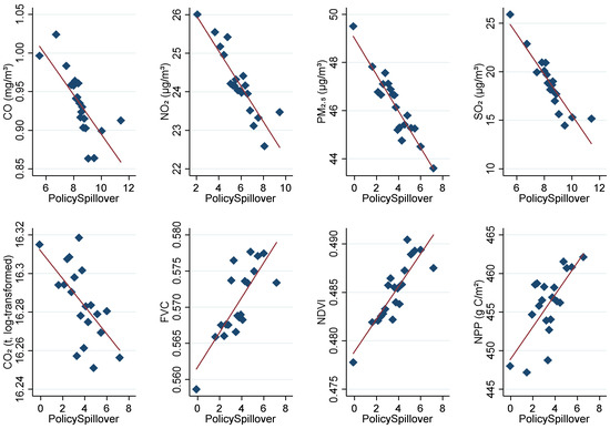
Figure 4.
The correlations between the “density of e-commerce development policy implementation in neighboring areas” and local environmental indicators during 2000–2021. Note: (1) Environmental quality is represented by eight indicators: carbon monoxide (CO), nitrogen dioxide (NO2), fine particulate matter (PM2.5), sulfur dioxide (SO2), carbon emission scale (CO2), fractional vegetation cover (FVC), normalized difference vegetation index (NDVI), and net primary productivity (NPP). (2) PolicySpillover measures the implementation density of e-commerce development policies in neighboring areas. It is a distance-weighted average of policy adoption in all regions other than the focal region itself, with weights equal to the inverse of the inter-regional distance. A detailed definition of this variable is provided in Section 3.2. (3) The binned scatter plots are drawn by using 20 bins. The graphs are similar if alternative bin numbers are selected. (4) Data sources are explained in detail in Section 3.3.
The eight subplots in the figure correspond to eight environmental quality indicators: carbon monoxide (CO), nitrogen dioxide (NO2), fine particulate matter (PM2.5), sulfur dioxide (SO2), total carbon emissions (CO2), fractional vegetation cover (FVC), normalized difference vegetation index (NDVI), and net primary productivity (NPP). The figure shows that if the density of e-commerce development policies in neighboring areas increases, the levels of CO, NO2, PM2.5, SO2, and carbon emission scale decrease, indicating a reduction in air pollution and carbon emissions; at the same time, FVC, NDVI and NPP increase, suggesting an improvement in vegetation greenness.
Based on the preliminary information provided in Figure 4, we can reasonably hypothesize that China’s e-commerce development policies have beneficial spatial spillover effects that improve environmental quality in neighboring regions. The core research hypothesis of this study is stated as follows:
Hypothesis 1 (H1).
China’s place-based e-commerce development policies generated beneficial spatial spillover effects on environmental quality in non-policy regions.
2.2.2. Possible Mechanisms
We also attempt to conduct mechanism analysis to explore through which channels e-commerce development policies affect environmental quality in other regions. We consider four potential mechanisms: industrial structure upgrading, technological progress, green innovation, and environmental regulation.
- (1)
- E-commerce may promote industrial structure upgrading in other regions. By integrating regional value chains, e-commerce enables different areas to engage in more refined specialization based on their comparative advantages. Furthermore, e-commerce platforms create a unified national market, intensifying competition among enterprises across regions and compelling them to transform. Industrial structure upgrading enhances the efficiency of economic activities, reducing resource consumption and waste, thereby improving environmental quality. Based on the above logic, we propose the following research hypothesis:
Hypothesis 2 (H2).
China’s place-based e-commerce development policies promoted industrial structure upgrading in non-policy regions.
- (2)
- E-commerce may promote technological progress in other regions. Development models and digital technologies from leading regions—such as platform architecture, big data analytics, and logistics algorithms—can diffuse to other areas through business cooperation, talent mobility, learning, and imitation. Such processes of technology spillover and knowledge dissemination facilitate technological advancement in other regions, thereby improving resource use efficiency and enhancing environmental quality. Therefore, we posit the following research hypothesis:
Hypothesis 3 (H3).
China’s place-based e-commerce development policies promoted technological progress in non-policy regions.
- (3)
- E-commerce may stimulate green innovation in other regions. In particular, both the BNEDC and CPZCE policies implemented in China explicitly emphasize promoting green economic development. As a result, local governments have adopted various economic and administrative measures to encourage enterprises to pursue energy conservation, emission reduction, and green innovation while developing e-commerce. Such policy demonstration effects and the spillover of green innovation technologies can enhance green innovation in non-policy regions, thereby contributing to energy saving, emission reduction, and improved environmental quality. We construct the following research hypothesis:
Hypothesis 4 (H4).
China’s place-based e-commerce development policies promoted green innovation in non-policy regions.
- (4)
- E-commerce may influence the stringency of environmental regulations in other regions. However, the direction of this effect is ambiguous. On the one hand, China’s e-commerce policies emphasize green development, which can help raise awareness of environmental protection and lead to stricter environmental regulations. On the other hand, governments may relax environmental regulations to reduce operational costs for businesses, enhancing regional competitiveness. To inspect the impact of e-commerce on environmental regulation, we will test the following research hypothesis:
Hypothesis 5 (H5).
China’s place-based e-commerce development policies strengthened environmental regulation in non-policy regions.
Figure 5 shows the conceptual model of this study. H1 is our core research hypothesis. To test it, we will ex post evaluate the impact of e-commerce development policies on the environmental quality of neighboring non-policy areas. H2 to H5 are the hypotheses formulated for mechanism analysis. We will separately examine the effects of e-commerce development policies on industrial structure upgrading, technological progress, green innovation, and environmental regulation in neighboring regions.
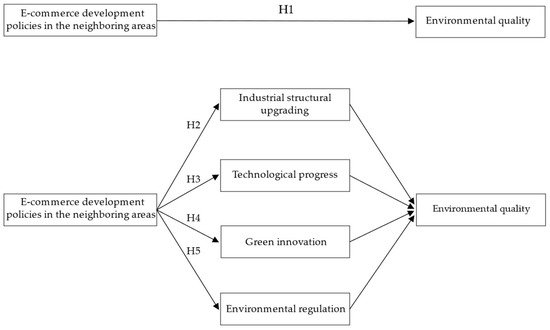
Figure 5.
Conceptual model of this study.
3. Materials and Methods
3.1. Empirical Model
This study aims to investigate the spatial spillover effects of China’s e-commerce development policies on the environment. Accordingly, in our empirical model, several environmental indicators serve as the explained variables (dependent variables). The core explanatory variable (independent variable) of interest is the implementation density of e-commerce development policies in neighboring regions. The model also includes a set of covariates (control variables), including factors representing meteorological conditions, local socioeconomic characteristics, and the implementation of other public policies.
To assess the spatial spillover effects of e-commerce development policies on environmental quality, this study relies on the following spatial econometric regression equation.
Y = ρWY + αPolicySpillover + Covariatesβ + s + v + u
u = λWu + ε
u = λWu + ε
Equation (1) is a Spatial Autoregressive Combined (SAC) Model. Appendix A provides a detailed explanation of our model selection process, justifying our choice of the SAC model. Equation (1) is a panel data regression model expressed in the form of matrix. A bolded letter denotes a matrix of variables or coefficients. Y is the vector of the explained variable; PolicySpillover is the vector of core explanatory variable of interest; Covariates the matrix of covariates; s represents region-fixed effects; v denotes time-fixed effects; ε is a vector of independently and identically distributed disturbance terms with zero mean. W is the spatial weights matrix. The scalar parameters ρ and λ measure the strength of dependence between different regions. α and β denote parameters for explanatory variables.
For a specific region i in period t, Equation (1) can be written as:
In Equation (2), the explained variable is Yit, which measures the environmental quality of region i in year t. The core explanatory variable of interest in this study is PolicySpilloverit = , representing the implementation density of e-commerce development policies in the neighboring regions of region i. In this variable, Wij denotes an element of a spatial weights matrix. EcommercePoliciesjt is a dummy variable indicating whether region j implemented at least one of the BNEDC or CPZCE policies in year t. Covariatesit represent a set of covariates. The definitions of these variables will be detailed in Section 3.2. si denotes the region-fixed effect, controlling for time-invariant region-specific characteristics (e.g., geographical location, cultural traditions). vt denotes the time-fixed effect, controlling for nationwide shocks (e.g., national environmental law reforms, pandemics). εit is the error term.
The coefficients α and β capture the effects of the corresponding explanatory variables on the explained variable. The values of these coefficients will be estimated using econometric regression methods, and their statistical significance will be assessed based on t-tests. α is the coefficient of particular interest in this study.
This coefficient α captures the extent to which the e-commerce development policies implemented in another region j affect the environmental quality in the local region i. If the coefficient α is statistically significant, it implies that, on average, the implementation of the policy in region j leads to a change in the environmental quality indicator Yit of region i by an amount equal to α (Wij × EcommercePoliciesjt). The total impact on region i from the policy implementation in all other regions j ≠ i is given by α. (It is worth noting that, due to the symmetry of the spatial weights matrix, the coefficient α also reflects the influence of the policy implemented in the local region i on another region j. If α is significant statistically, it means that, on average, the implementation of the policy in region i results in a change of α (Wji × EcommercePoliciesit) in the environmental quality indicator Yjt of region j.)
3.2. Variables
3.2.1. Explained Variables
The explained variable in Equation (1) is Yit, which represents environmental quality. Environmental quality is a multidimensional concept encompassing various aspects such as air, climate, water, soil, and vegetation. Due to data availability, we consider three dimensions of environmental quality.
- (1)
- Air quality, represented by four indicators: the concentrations of four air pollutants—CO, NO2, PM2.5, and SO2—in ambient air. Higher concentrations of these pollutants indicate more severe air pollution and poorer air quality.
- (2)
- Carbon emissions, represented by one indicator: the scale of total CO2 emissions. Excessive carbon emissions exacerbate global warming, trigger abnormal climate conditions, and negatively affect ecosystems and human health. Higher carbon emissions indicate poorer environmental quality. To mitigate heteroscedasticity issues in regression estimation, we apply the natural logarithm transformation to the carbon emission indicator.
- (3)
- Vegetation greenness, represented by three indicators: FVC, NDVI and NPP. Higher FVC and NDVI indicate greater vegetation cover density, while a higher NPP reflects more vigorous vegetation growth and stronger carbon sequestration capacity. Higher values of these indicators signify better vegetation conditions and higher environmental quality.
Table 1 reports the correlation coefficients between dependent variables. As can be seen from the table, these environmental indicators are highly correlated. Figure A1 in Appendix B uses histograms to show the empirical probability distributions of the eight dependent variables in this study. Figure A2 in Appendix B demonstrates the geographical distributions of these variables in China in 2020.

Table 1.
Correlation coefficient matrix of dependent variables.
3.2.2. Core Explanatory Variable
The core explanatory variable in Equation (1) is PolicySpilloverit = , which represents the implementation density of e-commerce development policies in the neighboring areas of region i. For region i, this variable is constructed by the weighted average of the e-commerce policy implementation status in all other regions j except region i itself, with the weight being the inverse of the geographical distance between regions i and j. Here, Wij is an element of the classical spatial weights matrix widely employed in spatial econometric literature, defined as follows:
where Distanceij denotes the straight-line geographical distance (in units of 100 km) between regions i and j. The distances between cities are calculated based on the latitude and longitude coordinates of their respective city centers.
As explained in the introduction section, given the similarity in content between the BNEDC and CPZCE policies and the high degree of overlap in their area coverage, we refer to both policies collectively as the “e-commerce development policy” and combine these two policies into a single policy category in the empirical analysis. The variable EcommercePoliciesjt is a binary dummy variable defined as follows: if region j implemented at least one of the BNEDC or CPZCE policies in year t, then EcommercePoliciesjt = 1; otherwise, EcommercePoliciesjt = 0.
Equation (3) is built on the following theoretical assumption: a public policy implemented in one region may exert influence on another region, and this influence is inversely proportional to the distance between two regions. In other words, in period t, the impact of region j’s implementation of the e-commerce development policies on region i is equal to α(Wij × EcommercePoliciesjt). Summing these influences over all regions j, i.e., α, yields the total effect of e-commerce development policies implemented in all other regions j ≠ i on the local region i.
To provide an intuitive illustration of the spatial spillover effects that this study attempts to measure—specifically, how the policy implemented in one region influences others—Figure 6 presents a simplified hypothetical example. Suppose there are three regions: i, j, and k. The distance between region i and j equals Distanceij = 1, and the distance between region k and j equals Distancekj = 2. Region j implements the e-commerce policies, but regions i and k do not. The policies implemented in region j generate spatial spillover effects, influencing both regions i and k. Since regions i and k do not implement the policies, they exert no influence on region j, nor do they affect each other. For region i, the policy spillover impact from region j is calculated as: α(Wij × EcommercePoliciesjt) = α × (1/Distanceij) × EcommercePoliciesjt = α × (1/1) × 1 = α. For region k, the policy spillover impact from region j is: α (Wkj × EcommercePoliciesjt) = α × (1/Distancekj) × EcommercePoliciesjt = α × (1/2) × 1 = α/2.
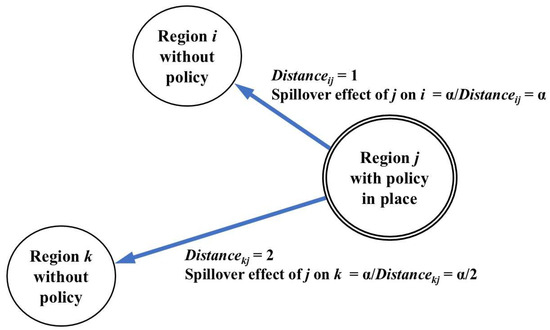
Figure 6.
Illustration of a policy’s spatial spillover effects depending on the inter-regional distances.
3.2.3. Covariates
To control for the influences of potential confounding factors, the regression equation incorporates a set of covariates. These covariates are divided into two groups. The first group includes nine meteorological and socioeconomic factors: precipitation, wind speed, temperature, GDP per capita, population density, share of the secondary industry, government size, financial development, and trade openness. The second group includes a composite index of place-based environmental policies and a composite index of place-based economic development policies. These two indices are used to represent thirty-three public policies implemented by the government that may affect regional environmental conditions. The descriptions of these covariates are provided in detail in Table 2. The list of the thirty-three place-based public policies are given in Table 3.
Table 2.
List of covariates.
Table 3.
List of thirty-three place-based public policies.
Admittedly, the chosen covariates are subject to potential limitations. Socioeconomic variables (e.g., GDP per capita, the proportion of the secondary industry, and trade openness) could be affected by the e-commerce policies, potentially contaminating the estimations of policy effects. Additionally, the covariates might be endogenous to the environmental outcomes, which introduces a risk of estimation bias. In light of these concerns that covariate selection might confound the empirical results, we will address this problem in our robustness check section.
3.3. Data Sources
The data used in this study were integrated from multiple sources. (1) Air pollution data, including CO, NO2, PM2.5, and SO2, were obtained from the GlobalHighAirPollutants (GHAP) dataset [37,38]. (2) Carbon emission data were obtained from the Emissions Database for Global Atmospheric Research (EDGAR) v8.0, provided by the European Union (EU). (3) FVC values were provided by Gao et al. [39]; NDVI values were derived from Li et al. [40]; and NPP values were obtained from NASA’s MOD17A3HGF product. The raw data for these environmental quality indicators were in the form of gridded data. After matching the raw data with the geographic location information of Chinese cities, we obtained annual values of the corresponding environmental quality indicators for each city in China. (4) Meteorological variable data were obtained from the ERA5-Land dataset offered by the EU’s Copernicus Climate Change Service. (5) Information on various public policies was collected from the official websites of relevant departments of the central government of China. (6) The remaining variables (such as GDP) were sourced from the EPS China database.
3.4. Research Sample
Based on data availability, this study utilizes annual-frequency data from 221 prefecture-level cities in mainland China spanning the 22-year period 2000–2021.
China has over 330 prefecture-level administrative districts and four provincial-level municipalities (i.e., Beijing, Tianjin, Shanghai, Chongqing). For simplicity, we refer to all of them as “cities” in this study. Among these cities, some have implemented the BNEDC and/or CPZCE policies, while others have not. Determining whether to include cities that have implemented e-commerce development policies in our study sample presents a difficult trade-off. On the one hand, including policy-implementing cities would increase our sample size by incorporating more cities, which is beneficial. On the other hand, including these cities introduces a considerable complication: the policy effect we aim to estimate would encompass three components—the direct effect of the locally implemented policies on the local area, the spillover effect of the locally implemented policies on other policy-implementing regions, and the spillover effect of the policies on non-policy regions. This would significantly complicate the empirical model. This situation poses a serious challenge to accurately assessing the policy effects, and to our knowledge, there is no sufficiently reliable empirical method in the existing literature to address such complex policy evaluation scenarios. Ultimately, to concentrate on analyzing the spatial spillover effects of e-commerce policies, we decide to exclude cities that had locally implemented the BNEDC and/or CPZCE policies. During the sample period, none of the included cities in this study had implemented either the BNEDC or CPZCE policy locally. Therefore, any influence of these policies on the sample cities stems entirely from spatial spillover effects. After excluding those policy-implementing cities, as well as cities with missing data, we retained 221 non-policy cities for analysis. Figure 7 shows the geographical locations of policy-implementing cities and the non-policy-implementing sample cities covered in this study. The map shows that our research covers nearly all non-policy cities in mainland China, ensuring a representative sample of the overall national context.
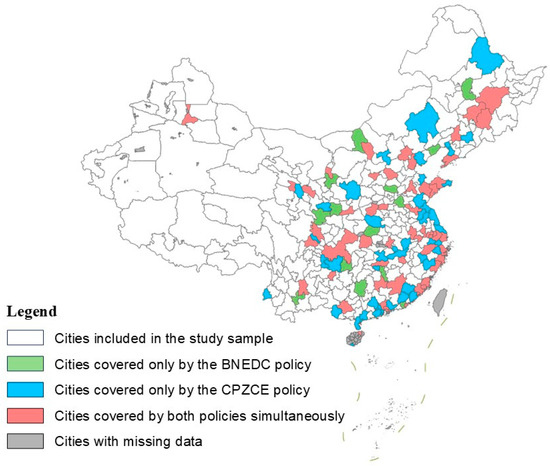
Figure 7.
The geographical distribution of cities implementing BNEDC and CPZCE policies and sample cities without policy implementation. Note: The green, blue, and red colors in the figure are based on the policy coverage in 2021, respectively representing “cities covered only by the BNEDC policy”, “cities covered only by the CPZCE policy”, and “cities covered by both policies simultaneously”. In earlier years, some cities had not yet implemented these policies. In the empirical analysis, we exclude from the research sample any cities that implemented the BNEDC and/or CPZCE policies by 2021, retaining only those cities that had never implemented the policies by 2021.
In our analysis of PM2.5, CO2 emissions, FVC, and NDVI, the research sample spans 22 years from 2000 to 2021. However, due to data availability constraints—specifically, the absence of CO and SO2 data prior to 2013, NO2 data before 2008, and NPP data for the years 2000 and 2021—the sample coverage varies when we analyze CO, SO2, NO2, and NPP. For CO and SO2, the sample covers 9 years (2013–2021); for NO2, it covers 14 years (2008–2021); for NPP, it covers 20 years (2001–2020).
Spatial econometric models require balanced panel data with no missing values. Therefore, before performing the regression analysis, we have filled the small number of missing values in the original data using interpolation. As a result, the final dataset constitutes a balanced panel. The number of observations ranges between 1989 and 4862, depending on the environmental indicator being analyzed. Descriptive statistics for key variables are reported in Table 4. Table A3 in Appendix C reports the changes in variables during the sample period.
Table 4.
Summary statistics of variables included in this study.
4. Results
In this section, we report the results of our empirical analysis. Section 4.1 presents the main findings of this study, i.e., the estimated spatial spillover impacts of e-commerce development policies on the environment. In Section 4.2, we investigate how far the policy impacts reach. In Section 4.3, we separately examine the impacts of the two policies, namely BNEDC and CPZCE. Section 4.4 verifies the robustness of the main findings. In Section 4.5 and Section 4.6, we conduct heterogeneity analysis and mechanism analysis, respectively. Section 4.7 provides a brief summary of the empirical results.
4.1. Main Results
Table 5 reports the coefficient estimation results for Equation (1) and, equivalently, Equation (2). In Panel A, we present the estimated effects of the e-commerce development policies on four air pollutants (including CO, NO2, PM2.5, and SO2). For all four pollutants, the estimated coefficients of the core explanatory variable, PolicySpilloverit, are negative and statistically significant.
Table 5.
Estimated coefficients of Equation (1).
In Panel B, we report the effects of the e-commerce development policies on carbon emissions and vegetation greenness. When the explained variable is the emission of CO2, the coefficients of PolicySpilloverit is significantly negative. When the explained variables are FVC, NDVI, and NPP, the coefficients of PolicySpilloverit are all significantly positive.
Table 5 also reports the coefficient estimates of the covariates. Factors such as rainfall, temperature, trade openness, and environmental policies also significantly affected environmental quality. Since these covariates are not the focus of our research, we do not discuss them in detail here.
It should be noted that our use of the SAC model allows for complex spatial interactions to exist among various variables across different regions. Therefore, the regression coefficients of PolicySpilloverit reported in Table 5 cannot be simply interpreted as the estimated magnitude of the policy spillover effects. Based on the spatial weights matrix we employ, we calculate the direct, indirect, and total effects of e-commerce development policies on the sample cities. (For a particular unit, the “direct effect” is the impact of a change in this unit’s own explanatory variable on its own explained variable. The “indirect effect” is the impact of this unit’s explanatory variable on the explained variables of other units. The “total effect” is the combined impact of this unit’s explanatory variable on all explained variables in the system, which equals the direct effect plus the indirect effect.) The total effect represents the ultimate magnitude of the policy spillover effect that we aim to assess.
The direct, indirect, and total effects of PolicySpilloverit are reported in Table 6. When the explained variables are air pollution and carbon emissions, the total effects are all significantly negative. This indicates that the e-commerce development policies significantly reduced air pollution and carbon emissions in non-policy areas, thereby improving their air quality and contributing to climate change mitigation. When the explained variables are indicators of vegetation greenness, the total effects are all significantly positive. This means that the e-commerce development policies enhanced vegetation greening in neighboring areas, improving vegetation coverage and promoting plant growth in these regions.
Table 6.
Estimated direct, indirect, and total effects on environment.
The results displayed in Table 6 explicitly demonstrate that the e-commerce development policies implemented in China have generated beneficial spatial spillover effects on the environment in non-policy areas. These effects benefited neighboring areas across three dimensions: air quality, climate change mitigation, and vegetation greening. Some previous studies have overlooked the spatial spillover influences of e-commerce development policies, thus underestimating the overall environmental benefits that such policies might generate.
The total effects of the policies reported in Table 6 are environmentally substantial. According to the values presented in the table, on average, a one-unit change in the PolicySpilloverit variable would lead to reductions of 0.174 mg/m3 for CO, 4.058 μg/m3 for NO2, 12.87 μg/m3 for PM2.5, and 25.03 μg/m3 for SO2. Simultaneously, CO2 emissions would decrease by 2.19%, while FVC, NDVI, and NPP would increase by 0.0321, 0.0144, and 39.40 gC/m2, respectively. The magnitude of these changes indicates significant environmental and public health benefits. It should be noted that the spatial econometric estimates are dependent on the spatial weights matrix we select. Different spatial weights matrices would yield different estimated total effects. However, as we will demonstrate later in the robustness check section, the policies’ total effects remain environmentally considerable if alternative spatial weights matrices are applied.
4.2. Detecting How Far the Policy Impacts Reach
Now, we try to detect how far the policy impacts reach. We modify Equation (1) by replacing the term PolicySpillover with three distance-binned spillover terms—PolicySpillover[0, 1000km], PolicySpillover(1000km, 1500km], and PolicySpillover(1500km, 2000km]—to obtain Equation (4).
Y = ρWY + α1PolicySpillover[0, 1000km] + α2PolicySpillover(1000km, 1500km]
+ α3PolicySpillover(1500km, 2000km] + Covariatesβ + s + v + u
u = λWu + ε
+ α3PolicySpillover(1500km, 2000km] + Covariatesβ + s + v + u
u = λWu + ε
The distance-binned spillover terms are employed to represent near, medium, and far away areas. This allows us to investigate over what distances the spillover effects of the e-commerce development policies could be observable. For a specific region i in period t, PolicySpilloverit[0, 1000km] = , PolicySpilloverit(1000km, 1500km] = , PolicySpilloverit(1500km, 2000km] = . The spatial weights matrix elements Wij[0, 1000km], Wij(1000km, 1500km], and Wij(1500km, 2000km] are defined as follows:
We estimate the coefficients of Equation (4) and calculate the total effects of PolicySpilloverit[0, 1000km], PolicySpilloverit(1000km, 1500km], and PolicySpilloverit(1500km,2000km], which are reported in Table 7. For CO, the total effect of PolicySpilloverit[0, 1000km] is significantly negative, whereas the total effects of PolicySpilloverit(1000km, 1500km] and PolicySpilloverit(1500km, 2000km] are not statistically significant. This indicates that the policy contributes to reducing CO pollution in areas within 1000 km, but has no discernible impact on regions beyond this range. The effective range of the policy’s spatial spillover effect on CO is approximately 1000 km.
Table 7.
Estimated spatial reach of policy effects.
Similarly, based on the results presented in the table, we find that the spatial spillover effect of the policy on PM2.5 extends to about 1000 km. For NO2, CO2, FVC, NDVI, and NPP, the spillover effects reach approximately 1500 km. Interestingly, for SO2, the spillover effect remains statistically significant even at distances as far as 2000 km.
In short, our findings demonstrate that the beneficial spatial spillover effects of the e-commerce policies on the environment can propagate over considerable distances—reaching at least 1000 km and in some cases much farther.
4.3. Respective Impacts of Two Policies
In the previous analysis, we combined BNEDC and CPZCE policies into a single policy variable EcommercePoliciesjt for empirical assessment. A potential concern is whether this approach obscures the differential effects of the BNEDC and CPZCE policies. To address this concern, we conduct an extended analysis by separating the two policies and estimating their environmental spillover effects individually. We construct BNEDCjt and CPZCEjt as binary dummy variables representing the BNEDC and CPZCE policies, respectively. BNEDCjt = 1 if region j implemented the BNEDC policy in year t, and BNEDCjt = 0 otherwise. Similarly, CPZCEjt = 1 if region j implemented the CPZCE policy in year t, and CPZCEjt = 0 otherwise. We then replace EcommercePoliciesjt in Equation (2) with these two dummy variables, constructing two terms: BNEDCSpilloverit = and CPZCESpilloverit = . By substituting these terms for PolicySpilloverit in Equation (2), we obtain Equation (8). We use Equation (8) to separately estimate the environmental spillover effects of the BNEDC and CPZCE policies.
Table 8 reports the estimates of total effects based on Equation (8). The results are as follows.
Table 8.
Estimated respective impacts of two policies.
- (1)
- When the dependent variables are NO2, PM2.5, and SO2 concentrations, the total effects of both terms BNEDCSpilloverit and CPZCESpilloverit are significantly negative. This indicates that both policies significantly reduced air pollution in non-policy regions, thereby improving air quality. It is noteworthy that when the dependent variable is CO, the total effects of both BNEDCSpilloverit and CPZCESpilloverit, while negative, are statistically nonsignificant. This may be because neither policy alone can produce a significant impact, and their simultaneous implementation is required to generate a significant spillover effect on CO.
- (2)
- When the dependent variable is the indicator of carbon emissions, the total effect of BNEDCSpilloverit is significantly negative, whereas the total effect of CPZCESpilloverit is negative but statistically nonsignificant. This suggests that the BNEDC policy did reduce carbon emissions in neighboring regions, while the CPZCE policy had no significant effect on carbon emissions in those areas.
- (3)
- When the dependent variable becomes FVC and NDVI, the total effect of BNEDCSpilloverit is positive but statistically nonsignificant, while the total effect of CPZCESpilloverit is significantly positive. When the dependent variable is NPP, the total effect of BNEDCSpilloverit is significantly positive, whereas the total effect of CPZCESpilloverit is positive but statistically nonsignificant. These results indicate that both policies contribute to some extent to the promotion of vegetation growth, though the specific effects depend on the measure of vegetation growth being considered.
Overall, the results in Table 8 reveal that the environmental spillover impacts of BNEDC and CPZCE are consistent qualitatively but differ in magnitude. Both policies demonstrate beneficial spatial spillover effects on the environment in other regions, though the specific extent of their impacts is not identical.
4.4. Robustness Checks
To confirm that the regression estimates based on Equation (1) are robust and not merely driven by a specific model specification, sample, or variable selection, we conduct six robustness checks.
In the first robustness test, we employ an alternative spatial weights matrix W0.5 to examine whether our results are sensitive to the choice of spatial weights. The elements of this matrix are defined in Equation (9):
In the second robustness test, we employ another alternative spatial weights matrix W[0, 1000km] to examine whether our results are sensitive to the choice of spatial weights. The elements of this matrix are already defined in Equation (5).
In the third robustness test, we exclude the samples before 2006. We do this because the scale of e-commerce transactions in China was quite small before 2006. By excluding the pre-2006 sample, we mitigate potential distortions that this nascent stage of e-commerce development could introduce into our analysis.
In the fourth robustness check, we winsorize all continuous variables at the 0.5th and 99.5th percentiles to mitigate potential distortions caused by possible outlier observations in the regression estimates.
In the fifth robustness check, we use one-year-lagged socioeconomic covariates in the regression estimates. We consider that some of these covariates (such as GDP per capita and population) may be endogenous to environmental outcomes, raising concerns about biased estimates. By lagging the covariates, we can mitigate the potential endogeneity issue caused by reverse causality, as environment in the current period cannot alter the covariates in the previous year.
In the sixth robustness test, we exclude the covariates Covariatesit from the regression model to examine whether the empirical results are sensitive to the selection of covariates.
The estimated total effects of PolicySpilloverit in these six robustness checks are reported in Rows (a) to (f) of Table 9, respectively. These findings are generally consistent with those presented in Table 6: the e-commerce development policies significantly reduced air pollution concentration and carbon emissions in non-policy regions, while increasing vegetation greenness.
Table 9.
Results of robustness checks.
4.5. Heterogeneity Analysis
In the preceding analysis, we treated all sample cities as homogeneous units and estimated the “average” spatial spillover effects of e-commerce development policies across all cities. However, spillover effects may vary among different cities. Focusing solely on average effects could obscure the heterogeneous impacts of the policy. For example, the eastern and central regions of China have a higher concentration of cities implementing e-commerce policies; cities with higher servicification levels and greater economic scales may be more responsive to e-commerce development policies; environmental conditions in densely populated urban areas may be more susceptible to change. In these regions, the spillover effects of e-commerce policies could be stronger. Therefore, we conduct a heterogeneity analysis to investigate whether the spillover influences of e-commerce development policies vary according to city characteristics.
We adopt the following empirical strategy for heterogeneity analysis. First, we choose a specific characteristic indicator and divide the sample cities into two groups—Group 1 and Group 2—based on the values of this indicator. We then define two dummy variables, DiGroup1 and DiGroup2, to indicate whether each city i belongs to Group 1 or Group 2. These dummy variables are defined as follows: if city i belongs to Group 1, then DiGroup1 = 1 and DiGroup2 = 0; if it belongs to Group 2, then DiGroup1 = 0 and DiGroup2 = 1. Next, we multiply these two dummy variables by PolicySpilloverit and obtain two interaction terms: PolicySpilloverit × DiGroup1 and PolicySpilloverit × DiGroup2. Subsequently, we replace PolicySpilloverit in Equation (2) with these two interaction terms to obtain Equation (10). The coefficients α1 and α2 in this equation capture the environmental spillover effects of the e-commerce development policies on cities belonging to Group 1 and Group 2, respectively.
We categorize the sample cities based on four types of characteristics. (1) By geographic location, we divide the cities into an eastern-central region group and a western region group. The results of the corresponding heterogeneity test are shown in Row (a) of Table 10. (2) Based on the average proportion of the tertiary industry in GDP during the sample period, cities are classified into a high servicification group and a low servicification group. The results of the heterogeneity test are recorded in Row (b) of Table 10. (3) Using the average GDP over the sample period, we group cities into a high economic scale group and a low economic scale group. The heterogeneity test results can be found in Row (c) of Table 10. (4) According to the average population density during the sample period, cities are divided into a high population density group and a low population density group. The results of the heterogeneity test are provided in Row (d) of Table 10.
Table 10.
Results of heterogeneity analysis.
The regression results reported in Table 10 show that, across different groups, the coefficients of the two interaction terms PolicySpilloverit × DiGroup1 and PolicySpilloverit × DiGroup2 are generally similar (though in a very few cases the coefficients are statistically nonsignificant). Therefore, the results of our heterogeneity tests actually indicate that the core findings of this study are highly robust. We observe beneficial spatial spillover impacts of e-commerce development policies on the environment across various types of cities, and no significant heterogeneity is detected.
Traditional theories of regional environmental policy analysis anticipate that policy effects will vary based on regional endowments and characteristics, such as industrial structure, human capital, and initial environmental quality [41,42]. However, our findings indicate that e-commerce development policies, as a form of digital technology-driven intervention, do not exhibit significant heterogeneity in their spatial spillover effects on the environment. This discovery diverges from the perspective of traditional theory. Our analytical results transcend the heterogeneity framework traditionally relied upon by conventional theories, which is based on local endowments and characteristics. In fact, our findings can find support in other relevant theories.
- (1)
- The literature on the “network effects” of technology diffusion suggests that once a technology matures and forms a network, its diffusion speed and pattern become relatively uniform, with minimal constraints from geographical distance [43,44]. E-commerce relies on the internet and logistics networks, both of which possess strong connectivity and standardization characteristics [45]. Once a region is integrated into such networks, the barriers and costs to accessing information, technology, and green business models (e.g., the sharing economy reducing resource wastes, optimized logistics routes lowering carbon emissions) are largely comparable to those in other regions. Therefore, the spillover of positive environmental externalities from e-commerce resembles a “network-based inclusive effect” rather than a “preferential effect” dependent on specific local conditions. Our robust results confirm that once digital technology diffusion surpasses a critical threshold, its positive impacts become widespread and uniform, demonstrating strong robustness in the effects observed.
- (2)
- The literature on “spatial integration” in new economic geography argues that reducing trade costs and information barriers can lead to a restructuring of economic spatial structures, forming a more efficient unified market [46,47]. E-commerce significantly lowers inter-regional information barriers and transaction costs [48], effectively creating a more integrated “digital common market”. Within this market, green technologies, products, and standards can diffuse across regions at lower costs, with their effectiveness less dependent on initial local conditions. For digital technology-driven policies, the spatial effects are universal, thus resulting in the robustness we observe in our findings.
4.6. Mechanism Analysis
We now proceed to conduct some mechanism analyses to explore through which channels e-commerce development policies affect environmental quality in other regions. As previously stated in the hypothesis development section, we consider four potential mechanisms: industrial structure upgrading, technological progress, green innovation, and environmental regulation.
- (1)
- Following previous studies [49,50], we construct an industrial structure upgrading index (ISUI), calculated as ISUI = I1 × 1 + I2 × 2 + I3 × 3, where I1, I2, and I3 represent the share of value-added from the primary, secondary, and tertiary industries in local GDP, respectively. A higher value of the ISUI indicates a greater degree of industrial structure upgrading. We replace the explained variable in Equation (1) with this index to estimate the impact of e-commerce policies on industrial structure upgrading in non-policy regions. The regression results are reported in Column (i) of Table 11. The total effect of PolicySpillover is significantly positive, indicating that e-commerce policies indeed significantly promoted industrial structure upgrading in non-policy regions.
Table 11. Results of mechanism analysis.
- (2)
- We measure technological progress by taking the logarithm of the number of patent applications plus one, and substitute this indicator as the explained variable in Equation (1). The regression results are recorded in Column (ii) of Table 11. The total effect of PolicySpillover is significantly positive, indicating that the e-commerce policies have indeed significantly promoted technological progress in non-policy regions.
- (3)
- We measure green innovation by taking the logarithm of the number of green patent applications plus one, and utilize this indicator to replace the explained variable in Equation (1). The regression results are shown in Column (iii) of Table 11. The significantly positive total effect of PolicySpillover indicates that the e-commerce policies have significantly promoted green innovation in non-policy regions.
- (4)
- Following previous research [51], we measure the stringency of environmental regulations using the proportion of environment-related terms in the text of the local government annual work reports. This indicator is used as the explained variable in Equation (1). The estimation results are shown in Column (iv) of Table 11. The total effect of PolicySpillover is statistically nonsignificant. We find no evidence that the e-commerce policies significantly altered the stringency of environmental regulations in non-policy regions.
In a nutshell, our mechanism analysis explored four potential channels. Although we did not observe significant changes in the stringency of environmental regulations, we found that the e-commerce policies significantly promoted industrial structure upgrading, technological progress, and green innovation in neighboring regions. These findings provide a plausible explanation for the core finding of this study—e-commerce development policies generated beneficial spatial spillover effects on the environment.
4.7. Summary of Empirical Results
We now provide a concise summary of the empirical results, which are encapsulated in Table 12. (1) We begin by verifying that the e-commerce development policies exerted significant beneficial impacts on the environment of non-policy areas. Our results show that the policies improved air quality, reduced carbon emissions, and increased vegetation greenness in neighboring regions. (2) Our analysis detects that the spatial reach of the policy effects spanned a distance of approximately 1000 to 1500 km. (3) We separately estimate the effects of the BNEDC and CPZCE policies. The results demonstrate that both policies contributed to improved environmental quality in non-policy areas. (4) Robustness checks conducted on our core findings confirm that the results hold under various model specifications, samples, and variable choices. (5) Heterogeneity analysis reveals that the policy effects are largely consistent across regions with different characteristics, showing no obvious heterogeneity. (6) Mechanism analysis indicates that the policies achieved their impacts by facilitating industrial structure upgrading, accelerating technological progress, and stimulating green innovation.
Table 12.
Summary of empirical results.
5. Discussion
This study empirically analyzes the spatial spillover effects of two e-commerce development policies in China—the “Building National E-commerce Demonstration Cities” and the “Comprehensive Pilot Zones for Cross-Border E-commerce”—on environmental quality. The findings indicate that these policies generated significant positive environmental impacts on non-policy areas. Hypothesis 1 of this study is clearly supported. Furthermore, we analyze the potential mechanisms through which the policies exert their effects. The results indicate that e-commerce development policies promoted industrial structure upgrading, technological progress, and green innovation in non-policy regions. Hypotheses 2, 3, and 4 are all supported. However, we do not find evidence that these policies enhanced environmental regulation in neighboring areas. Thus, Hypothesis 5 is not supported. These results extend the current understanding of the environmental effects of e-commerce policies and offer a new policy perspective for regional coordinated emission reduction and green development.
5.1. Academic Implications
The major academic contribution of this study lies in revealing that well-designed e-commerce policies can generate positive environmental externalities across regions. Through channels such as green upgrading of industrial chains, diffusion of low-carbon technologies, and innovation spillovers, e-commerce policies can drive improvements in multiple environmental indicators in non-policy areas. This finding breaks through the traditional mindset of confining policy evaluation to policy-implementing regions. This provides empirical support from the digital economy sector for theories on policy externalities and spatial spillovers in “New Economic Geography” and environmental economics. Our findings emphasize the necessity of incorporating spatial dimensions into the evaluation of e-commerce development policies. Our study also alerts future researchers that relying solely on traditional difference-in-differences (DID) methods to assess policy effects may be biased, as the key assumption of “no spatial spillover effects” might not hold. Understanding the potential spatial interactions among various factors is indispensable for comprehensive policy evaluation, as advocated by spatial economics [52,53,54].
Furthermore, the heterogeneity test results in this study indicate that the policy spillover effects are significantly present across various types of cities, transcending geographical, economic, or demographic constraints. This demonstrates that the green transition driven by e-commerce possesses broad adaptability and inclusivity, and a well-designed economic policy can generate positive externalities even in diverse local contexts. This insight holds value for developing theories on coordinated regional development.
5.2. Practical Implications
The findings of this research offer practical references for both central and local governments in formulating policies that synergistically promote economic development and environmental protection.
First, the “point-to-area” regional coordinated governance model is worth exploring. Given that certain economic policies generate beneficial spatial spillover effects, adopting a “pilot-then-scale” approach based on careful policy impact assessments could effectively enhance social welfare. In policy design, strategically selected “key node” cities can serve as pilot zones, leveraging their technological diffusion, industrial transfer, and green innovation spillovers to drive sustainable development across entire regional clusters. In this way, the impacts of local pilot programs can be leveraged to generate public interests across a wider region [55]. While this governance approach has been practiced in China for many years, it remains underutilized in some other developing countries. Other nations could learn from China’s “pilot-then-scale” model to implement public policies with lower governance costs.
Second, the design of China’s e-commerce development policies could be optimized to strengthen positive spillover channels. The presence of beneficial spatial spillovers may create free-rider incentives, where some regions benefit from others’ efforts without contributing themselves. Such behavior can undermine collective welfare and reduce the motivation of policy-implementing areas to share outcomes. This should be avoided. When introducing e-commerce-related industrial support policies, local governments should look beyond narrow local interests and consider “whether regional positive externalities can be generated” as a key evaluation criterion. To incentivize proactive efforts, the central government could consider providing additional rewards to top-performing regions. Policy design should more deliberately encourage key cities to establish green technology cooperation platforms and jointly develop low-carbon industrial chains and supply chains with neighboring areas, thereby transforming spatial spillovers from “spontaneous” to “organized” actions and maximizing regional synergistic benefits.
Third, policy efforts should be clearly focused on core mechanisms through which spillovers operate. The mechanism analysis of this study indicates that the spatial spillover effects of policies work primarily by stimulating intrinsic market dynamics rather than through heightened administrative regulations. From the perspectives of economic structural transformation and technological innovation, several previous studies have emphasized that industrial structural upgrading and technological progress exert significant spatial spillover effects on energy intensity and carbon emissions [56,57]. From the perspective of green development, Peng et al. [58] demonstrated that green innovation has a significantly positive spatial spillover influence on the quality of economic development in China. Therefore, future policy priorities should continue to emphasize incentivizing technological development, supporting the growth of service and high-tech manufacturing industries, encouraging green innovation, and providing incentives for low-carbon energy transition. By fostering new drivers of economic growth, environmental goals can be achieved indirectly yet more sustainably.
6. Conclusions, Limitations, and Future Research Directions
6.1. Conclusions
Based on the findings of this study, it can be concluded that China’s two crucial e-commerce development policies—namely the “Building National E-Commerce Demonstration Cities” and “Comprehensive Pilot Zones for Cross-Border E-Commerce”—generated significant beneficial spatial spillover effects on the environment in non-policy areas. The policies not only reduced air pollution (including CO, NO2, PM2.5, and SO2) in neighboring regions but also led to decreased carbon emissions and increased vegetation greenness in these regions. The spillover effects were consistently observed across cities with different geographic locations, industrial structures, economic scale, and population densities. Mechanism analysis confirms that the spillover effects were primarily driven by industrial upgrading, technological progress, and green innovation in non-policy areas, rather than changes in environmental regulation.
This study underscores the important role of e-commerce development policies in generating broad environmental benefits beyond their targeted regions, providing empirical support for integrated regional policy design that leverages well-designed e-commerce growth as a tool for ecological improvement.
6.2. Limitations
Our research has several limitations. In the future, researchers could further analyze the environmental effects of e-commerce by addressing these shortcomings. (1) Due to data constraints, our research sample period ended in 2021. Our study does not explore developments after 2022. In recent years, new information technologies such as big data, artificial intelligence, and large language models have continued to emerge and have seen increased development and application. These advancements have further facilitated the expansion of e-commerce. (2) As we lack more granular data on the specific types of e-commerce businesses in each city, this study treats the e-commerce development across all cities as a homogeneous category, thereby simply capturing an average effect. (3) Our research is based on the context of China. We have not verified whether our findings are applicable to other countries. Given that China has a relatively distinctive institutional, market, and policy environment, and that institutional settings, market structures, and energy compositions may vary across countries, it remains uncertain whether the conclusions of this study are generalized to other nations.
6.3. Future Research Directions
Based on the aforementioned limitations of this study, future research can be further expanded and improved in the following aspects to deepen the understanding of the environmental and spatial spillover effects of e-commerce.
- (1)
- Collecting more updated and multidimensional data. Future studies could utilize more recent and diverse data sources, such as satellite remote sensing data, online transaction data from e-commerce platforms, and logistics route data, to verify the robustness of the conclusions presented in this paper.
- (2)
- Distinguishing between different types and industries of e-commerce. Future research may further classify e-commerce models to allow for an examination of the differences among their environmental effects. For instance, in terms of business models, comparisons can be made among business-to-business (B2B), business-to-consumer (B2C), and consumer-to-consumer (C2C) transactions to determine whether their environmental impacts differ. From an industry perspective, e-commerce in different sectors, such as agriculture, manufacturing, and services, may exhibit distinct environmental influences.
- (3)
- Incorporating an international perspective. Given the cross-country differences in economic development levels, infrastructure conditions, energy structures, regulatory intensity, and digital governance capacity, the environmental consequences of e-commerce may vary across nations. For example, developed countries have accumulated experience in areas such as green logistics, circular packaging, and sustainable supply chains, while many developing countries are still in the early stages of building digital infrastructure. Future researchers could build on our analytical framework to explore the environmental influences of e-commerce in other economies. This issue is particularly important for countries with large populations—and thus significant e-commerce potential—that also face severe environmental challenges, such as Bangladesh, India, Indonesia, Nigeria, and Pakistan.
Author Contributions
Conceptualization, D.D.; methodology, D.D.; data curation, D.Z. and D.D.; formal analysis, D.Z. and D.D.; software, D.Z. and D.D.; validation, D.Z. and D.D.; visualization, D.Z. and D.D.; writing—original draft, D.Z. and D.D.; writing—review and editing, D.Z. and D.D. All authors have read and agreed to the published version of the manuscript.
Funding
This research received no external funding.
Institutional Review Board Statement
Not applicable.
Informed Consent Statement
Not applicable.
Data Availability Statement
The data supporting the findings of this study were obtained from publicly available sources cited throughout the article. All data sources are explicitly referenced in the article.
Conflicts of Interest
The authors declare no conflicts of interest.
Appendix A. Procedures of Model Selection
Appendix A.1. Assessing the Suitability of the Two-Way Fixed Effects Regression Model
We begin by assuming that, aside from the spatial spillover effects of the e-commerce development policies, there are no spatial spillover effects from other variables. Under this assumption, we can estimate the spillover effects of the e-commerce development policies using the following two-way fixed effects (TWFE) panel data regression equation.
Yit = αPolicySpilloverit + Covariatesitβ + si + vt + εit
After obtaining the coefficient estimates, we calculate the Moran’s I values of the regression residuals. The Moran’s I values are reported in Table A1. The results show that the Moran’s I values are statistically significant overall, implying the presence of considerable spatial autocorrelation in the residuals. Therefore, the TWFE model is insufficient to fully capture the complex relationships among the variables, making it necessary for us to consider employing spatial econometric models for further analysis.
Table A1.
Moran’s I for residuals from two-way fixed effects regression estimations.
Table A1.
Moran’s I for residuals from two-way fixed effects regression estimations.
| Year | CO | NO2 | PM2.5 | SO2 | ||||
| Moran’s I | z Statistic | Moran’s I | z Statistic | Moran’s I | z Statistic | Moran’s I | z Statistic | |
| 2000 | - | - | - | - | 0.291 *** | 34.339 | - | - |
| 2001 | - | - | - | - | 0.303 *** | 35.746 | - | - |
| 2002 | - | - | - | - | 0.273 *** | 32.208 | - | - |
| 2003 | - | - | - | - | 0.268 *** | 31.776 | - | - |
| 2004 | - | - | - | - | 0.240 *** | 28.474 | - | - |
| 2005 | - | - | - | - | 0.230 *** | 27.308 | - | - |
| 2006 | - | - | - | - | 0.182 *** | 21.714 | - | - |
| 2007 | - | - | - | - | 0.222 *** | 26.345 | - | - |
| 2008 | - | - | 0.186 *** | 22.200 | 0.210 *** | 25.042 | - | - |
| 2009 | - | - | 0.164 *** | 19.565 | 0.166 *** | 19.799 | - | - |
| 2010 | - | - | 0.090 *** | 10.971 | 0.15 *** | 18.085 | - | - |
| 2011 | - | - | 0.142 *** | 17.047 | 0.186 *** | 22.133 | - | - |
| 2012 | - | - | 0.087 *** | 10.631 | 0.237 *** | 28.065 | - | - |
| 2013 | 0.117 *** | 14.155 | 0.149 *** | 17.827 | 0.228 *** | 26.998 | 0.113 *** | 13.715 |
| 2014 | 0.098 *** | 11.897 | 0.136 *** | 16.364 | 0.252 *** | 29.754 | 0.137 *** | 16.584 |
| 2015 | 0.108 *** | 13.146 | 0.100 *** | 12.202 | 0.197 *** | 23.437 | 0.065 *** | 8.066 |
| 2016 | 0.128 *** | 15.400 | 0.089 *** | 10.934 | 0.199 *** | 24.533 | 0.100 *** | 12.306 |
| 2017 | 0.076 *** | 9.427 | 0.076 *** | 9.348 | 0.102 *** | 12.442 | 0.136 *** | 16.520 |
| 2018 | 0.077 *** | 9.519 | 0.110 *** | 13.344 | 0.132 *** | 15.921 | 0.090 *** | 11.051 |
| 2019 | 0.132 *** | 15.856 | 0.128 *** | 15.410 | 0.104 *** | 12.650 | 0.111 *** | 13.425 |
| 2020 | 0.143 *** | 17.142 | 0.099 *** | 11.980 | 0.100 *** | 12.149 | 0.161 *** | 19.250 |
| 2021 | 0.166 *** | 19.830 | 0.153 *** | 18.363 | 0.141 *** | 16.902 | 0.101 *** | 12.3109 |
| Year | CO2 | FVC | NDVI | NPP | ||||
| Moran’s I | z statistic | Moran’s I | z statistic | Moran’s I | z statistic | Moran’s I | z statistic | |
| 2000 | −0.013 | −1.055 | 0.1773 *** | 21.141 | 0.170 *** | 20.317 | - | - |
| 2001 | −0.014 | −1.073 | 0.1669 *** | 19.928 | 0.190 *** | 22.583 | 0.180 *** | 21.460 |
| 2002 | −0.014 | −1.102 | 0.186 *** | 22.129 | 0.206 *** | 24.540 | 0.147 *** | 17.609 |
| 2003 | −0.013 | −1.033 | 0.148 *** | 17.694 | 0.120 *** | 14.480 | 0.155 *** | 18.642 |
| 2004 | −0.011 | −0.789 | 0.050 *** | 6.406 | 0.137 *** | 16.471 | 0.229 *** | 27.213 |
| 2005 | 0.054 *** | 6.957 | 0.200 *** | 23.871 | 0.080 *** | 9.829 | 0.197 *** | 23.511 |
| 2006 | 0.055 *** | 7.104 | 0.071 *** | 8.783 | 0.032 *** | 4.215 | 0.118 *** | 14.268 |
| 2007 | 0.049 *** | 6.369 | 0.157 *** | 18.845 | 0.167 *** | 19.935 | 0.169 *** | 20.135 |
| 2008 | 0.010 * | 1.796 | 0.157 *** | 18.788 | 0.206 *** | 24.478 | 0.174 *** | 20.770 |
| 2009 | 0.014 ** | 2.254 | 0.180 *** | 21.472 | 0.111 *** | 13.408 | 0.157 *** | 18.787 |
| 2010 | 0.013 ** | 2.235 | 0.147 *** | 17.579 | 0.154 *** | 18.436 | 0.14 *** | 16.854 |
| 2011 | −0.001 | 0.427 | 0.136 *** | 16.411 | 0.162 *** | 19.456 | 0.128 *** | 15.421 |
| 2012 | −0.007 | −0.275 | 0.253 *** | 30.012 | 0.094 *** | 11.528 | 0.183 *** | 21.905 |
| 2013 | 0.020 *** | 2.919 | 0.149 *** | 17.845 | 0.157 *** | 18.767 | 0.165 *** | 19.753 |
| 2014 | 0.020 *** | 3.088 | 0.125 *** | 15.124 | 0.095 *** | 11.660 | 0.146 *** | 17.495 |
| 2015 | 0.012 ** | 2.082 | 0.163 *** | 19.515 | 0.156 *** | 18.617 | 0.198 *** | 23.602 |
| 2016 | 0.006 | 1.290 | 0.184 *** | 21.909 | 0.108 *** | 13.036 | 0.170 *** | 20.322 |
| 2017 | 0.017 ** | 2.548 | 0.118 *** | 14.290 | 0.103 *** | 12.525 | 0.099 *** | 11.997 |
| 2018 | 0.024 *** | 3.337 | 0.163 *** | 19.542 | 0.146 *** | 17.664 | 0.124 *** | 14.920 |
| 2019 | 0.026 *** | 3.565 | 0.174 *** | 20.807 | 0.124 *** | 14.896 | 0.181 *** | 21.620 |
| 2020 | 0.020 *** | 2.835 | 0.126 *** | 15.184 | 0.101 *** | 12.280 | 0.127 *** | 15.253 |
| 2021 | 0.026 *** | 3.590 | 0.123 *** | 14.808 | 0.093 *** | 11.399 | - | - |
Note: ***, **, and * represent statistical significance at the 1%, 5%, and 10% levels, respectively.
Appendix A.2. Selecting Spatial Econometric Regression Models
There are multiple spatial econometric regression models available for panel data analysis, such as the SAC (Spatial Autoregressive Combined Model), SDM (Spatial Durbin Model), SAR (Spatial Autoregressive Model), and SEM (Spatial Error Model). Since the SAC and SDM models are more generalized, we begin by comparing these two models.
The SAC model can be represented by the following equation:
where Y is the vector of the explained variable; X is the matrix of explanatory variables; s represents region-fixed effects; v denotes time-fixed effects; ε is a vector of independently and identically distributed disturbance terms with zero mean. W is the spatial weights matrix. The scalar parameters ρ and λ measure the strength of dependence between different regions. β is a vector of parameters for explanatory variables.
Y = ρWY + Xβ + s + v + u
u = λWu + ε
u = λWu + ε
The SDM can be expressed by the following equation:
θ is a vector of parameters measure the spatial spillover effects of explanatory variables. The meanings of other variables and parameters are the same as those in the aforementioned SAC model.
Y = ρWY + Xβ + WXθ + s + v + ε
We put the explained and explanatory variables of this study into the SAC and SDM equations, estimate the coefficients, and obtain the corresponding Akaike Information Criterion (AIC) and Bayesian Information Criterion (BIC) values for both models. The AIC and BIC values are reported in Table A2. Models with lower AIC and BIC values are preferred [59]. As shown in the table, except for the case where the dependent variable is CO2, the SAC model has lower AIC and BIC values than the SDM model in the other seven scenarios with different dependent variables. Therefore, overall, the SAC model should be preferred over the SDM model.
Next, we compare the SAC model and the SAR model. The SAR model can be expressed by the following equation:
Y = ρWY + Xβ + s + v + ε
In other words, when the parameter λ in the SAC model is constrained to λ = 0, the SAC model simplifies to the SAR model. We use the likelihood ratio (LR) test to determine whether the SAR model should be selected. The test results support the SAC model over the SAR model.
Then, we compare the SAC model and the SEM model. The SEM model can be represented by the following equation:
Y = Xβ + s + v + u
u = λWu + ε
u = λWu + ε
That is, when we restrict the parameter ρ in the SAC model to ρ = 0, the SAC model simplifies to the SEM model. We employ the likelihood ratio test to determine whether the SEM model should be selected. The test results support the SAC model over the SEM model.
In summary, we have compared four commonly used spatial econometric models, including SAC, SDM, SAR, and SEM. The statistical test results support the selection of the SAC model. Therefore, we utilize the SAC model to analyze the spatial spillover effects of e-commerce policies on the environment.
Table A2.
AIC and BIC values of SAC and SDM models.
Table A2.
AIC and BIC values of SAC and SDM models.
| Model | CO | NO2 | PM2.5 | SO2 | ||||
| AIC | BIC | AIC | BIC | AIC | BIC | AIC | BIC | |
| SAC | 9.94 | 93.87 | 10,805.86 | 10,896.41 | 22,915.38 | 23,012.72 | 9060.76 | 9142.92 |
| SDM | 29.94 | 169.83 | 10,875.79 | 11,026.72 | 23,993.86 | 24,156.09 | 9115.01 | 9251.95 |
| Model | CO2 | FVC | NDVI | NPP | ||||
| AIC | BIC | AIC | BIC | AIC | BIC | AIC | BIC | |
| SAC | −7168.05 | −7070.72 | −25,115.73 | −25,018.39 | −29,723.88 | −29,626.54 | 40,215.95 | 40,311.86 |
| SDM | −7252.35 | −7090.12 | −24,500.88 | −24,338.65 | −29,439.61 | −29,277.38 | 40,992.48 | 41,152.33 |
Abbreviations: Akaike Information Criterion (AIC); Bayesian Information Criterion (BIC); Spatial Autoregressive Combined Model (SAC), Spatial Durbin Model (SDM).
Appendix B. The Distributions of the Dependent Variables
Figure A1 uses histograms to show the empirical probability distributions of the eight dependent variables in this study. Figure A2 demonstrates the geographical distributions of these variables in China in 2020.

Figure A1.
The empirical probability distributions of the dependent variables.
Figure A1.
The empirical probability distributions of the dependent variables.


Figure A2.
The geographical distributions of the dependent variables in China in 2020. Note: Subfigures (a–h) show the circumstances of CO, NO2, PM2.5, SO2, CO2, FVC, NDVI, and NPP, respectively.
Figure A2.
The geographical distributions of the dependent variables in China in 2020. Note: Subfigures (a–h) show the circumstances of CO, NO2, PM2.5, SO2, CO2, FVC, NDVI, and NPP, respectively.


Appendix C. The Changes in Variables During the Sample Period
Table A3.
The changes in variables during the sample period.
Table A3.
The changes in variables during the sample period.
| Variables | Mean at the Start of the Sample Period | Mean at the End of the Sample Period | Absolute Change from the Start to the End of the Sample Period | Percentage Change from the Start to the End of the Sample Period | Mean Annual Absolute Change | Mean Annual Percentage Change (Arithmetic Mean) | Mean Annual Percentage Change (Geometric Mean) |
|---|---|---|---|---|---|---|---|
| CO | 1.174 | 0.675 | −0.499 | −42.5% | −0.062 | −5.3% | −6.7% |
| NO2 | 24.702 | 18.187 | −6.515 | −26.4% | −0.501 | −2.0% | −2.3% |
| PM2.5 | 42.516 | 29.504 | −13.012 | −30.6% | −0.620 | −1.5% | −1.7% |
| SO2 | 30.381 | 10.045 | −20.335 | −66.9% | −2.542 | −8.4% | −12.9% |
| CO2 | 15.568 | 16.658 | 1.090 | 7.0% | 0.052 | 0.3% | 0.3% |
| NDVI | 0.469 | 0.515 | 0.046 | 9.8% | 0.002 | 0.5% | 0.4% |
| FVC | 0.527 | 0.626 | 0.099 | 18.7% | 0.005 | 0.9% | 0.8% |
| NPP | 408.707 | 489.363 | 80.656 | 19.7% | 4.245 | 1.0% | 1.0% |
| PolicySpillover | 0.000 | 13.324 | 13.324 | - | 0.634 | - | - |
| Precipitation | 0.843 | 0.929 | 0.086 | 10.1% | 0.004 | 0.5% | 0.5% |
| WindSpeed | 2.486 | 2.516 | 0.030 | 1.2% | 0.001 | 0.1% | 0.1% |
| Temperature | 11.053 | 12.151 | 1.098 | 9.9% | 0.052 | 0.5% | 0.5% |
| GDPPerCapita | 8.474 | 10.199 | 1.725 | 20.4% | 0.082 | 1.0% | 0.9% |
| PopulationDensity | 0.273 | 0.304 | 0.031 | 11.2% | 0.001 | 0.5% | 0.5% |
| SecondaryIndustry | 0.386 | 0.381 | −0.006 | −1.5% | 0.000 | −0.1% | −0.1% |
| GovernmentSize | 0.125 | 0.298 | 0.173 | 138.5% | 0.008 | 6.6% | 4.2% |
| FinancialDevelopment | 0.829 | 1.119 | 0.290 | 35.0% | 0.014 | 1.7% | 1.4% |
| TradeOpenness | 0.109 | 0.174 | 0.066 | 60.4% | 0.003 | 2.9% | 2.3% |
| EnvironmentalPolicies | 0.002 | 0.281 | 0.279 | 12525.3% | 0.013 | 596.4% | 25.9% |
| EconomicPolicies | 0.000 | 0.241 | 0.241 | - | 0.011 | - | - |
References
- Abdulkarem, A.; Hou, W. The impact of organizational context on the levels of cross-border e-commerce adoption in Chinese SMEs: The moderating role of environmental context. J. Theor. Appl. Electron. Commer. Res. 2021, 16, 2732–2749. [Google Scholar] [CrossRef]
- Liu, A.; Osewe, M.; Shi, Y.; Zhen, X.; Wu, Y. Cross-border e-commerce development and challenges in China: A systematic literature review. J. Theor. Appl. Electron. Commer. Res. 2022, 17, 69–88. [Google Scholar] [CrossRef]
- Sun, X.; Huang, Q.; Zhang, H.; Zhao, X. Comprehensive pilot zones for cross-border E-commerce propel the digital transformation of manufacturing enterprises: New evidence from China. Electron. Commer. Res. 2024. [Google Scholar] [CrossRef]
- Yao, T.; Qiu, Z. Can e-commerce narrow regional economic disparities? Evidence from national e-commerce demonstration cities policy in China. GeoJournal 2024, 89, 165. [Google Scholar] [CrossRef]
- Liu, D.; Qiu, Z. Can e-commerce reduce urban CO2 emissions? Evidence from National E-commerce Demonstration Cities policy in China. Environ. Sci. Pollut. Res. 2023, 30, 58553–58568. [Google Scholar] [CrossRef]
- Zhou, C.; Li, B. How does e-commerce demonstration city improve urban innovation? Evidence from China. Econ. Transit. Institutional Change 2023, 31, 915–940. [Google Scholar] [CrossRef]
- Shenzhen Municipal People’s Government. Notice of the Shenzhen Municipal People’s Government on Issuing the Development Plan for Reinvigorating the Internet Industry in Shenzhen (2009–2015). 2009. Available online: https://www.sz.gov.cn/zfgb/2010/gb681/content/post_4999761.html (accessed on 1 September 2025).
- The State Council of the People’s Republic of China. State Council Approval on the Establishment of the China (Hangzhou) Comprehensive Pilot Zone for Cross-Border E-commerce. 2015. Available online: https://www.gov.cn/gongbao/content/2015/content_2838169.htm (accessed on 1 September 2025).
- Jiang, P.; Qin, S. E-commerce empowers urban entrepreneurial activity—Empirical evidence from the construction of national e-commerce demonstration cities. Cities 2024, 150, 105092. [Google Scholar] [CrossRef]
- Pan, X.; Zhou, C. The impact of e-commerce city pilot on the spatial agglomeration of high-end service industry in China. Int. Stud. Econ. 2023, 18, 326–350. [Google Scholar] [CrossRef]
- Wang, W.; Sun, M.; Zhou, D. The impact of cross-border e-commerce comprehensive pilot zone on corporate financial constraints in China. Humanit. Soc. Sci. Commun. 2025, 12, 1107. [Google Scholar] [CrossRef]
- Manta, A.G.; Doran, N.M.; Hurduzeu, G.; Bădîrcea, R.M.; Doran, M.D.; Manta, F.L. Is there a direct benefit of using electronic commerce and electronic banking in mitigating climate change? Clim. Change 2024, 177, 152. [Google Scholar] [CrossRef]
- Xie, H.; Chang, S.; Wang, Y.; Afzal, A. The impact of e-commerce on environmental sustainability targets in selected European countries. Econ. Res.-Ekon. Istraživanja 2023, 36, 230–242. [Google Scholar] [CrossRef]
- Liu, X.; Cui, W.; Zhang, S. Better e-commerce less carbon emissions in China? Energy 2025, 318, 134820. [Google Scholar] [CrossRef]
- Chen, W.; Yan, W. Impact of internet electronic commerce on SO2 pollution: Evidence from China. Environ. Sci. Pollut. Res. 2020, 27, 25801–25812. [Google Scholar] [CrossRef] [PubMed]
- Yu, W.; Wu, Y.; Tan, X.; Guo, X. The nexus between electronic commerce and environmental pollution: The roles of energy efficiency and resource consumption. Bus. Strategy Environ. 2024, 33, 2287–2300. [Google Scholar] [CrossRef]
- Bjerkan, K.Y.; Bjørgen, A.; Hjelkrem, O.A. E-commerce and prevalence of last mile practices. Transp. Res. Procedia 2020, 46, 293–300. [Google Scholar] [CrossRef]
- Le, H.T.K.; Carrel, A.L.; Shah, H. Impacts of online shopping on travel demand: A systematic review. Transp. Rev. 2021, 42, 273–295. [Google Scholar] [CrossRef]
- Kemp, R.; Volpi, M. The diffusion of clean technologies: A review with suggestions for future diffusion analysis. J. Clean. Prod. 2008, 16, S14–S21. [Google Scholar] [CrossRef]
- Ali, S.A.S.; Ilankoon, I.M.S.K.; Zhang, L.; Tan, J. Packaging plastic waste from e-commerce sector: The Indian scenario and a multi-faceted cleaner production solution towards waste minimisation. J. Clean. Prod. 2024, 447, 141444. [Google Scholar] [CrossRef]
- Kim, Y.; Kang, J.; Chun, H. Is online shopping packaging waste a threat to the environment? Econ. Lett. 2022, 214, 110398. [Google Scholar] [CrossRef]
- Okubo, T.; Picard, P.M.; Thisse, J. The spatial selection of heterogeneous firms. J. Int. Econ. 2010, 82, 230–237. [Google Scholar] [CrossRef]
- Liu, Y.; Zhang, M.; Fan, B.; Fu, S.; Liu, Y. The green side of digital trade: Evaluating the impact of National E-commerce Demonstration Cities policy. Int. Rev. Econ. Financ. 2025, 99, 104071. [Google Scholar] [CrossRef]
- Qiao, L.; Huo, D.; Sun, T.; Zhao, Z.; Ma, L.; Wu, Z. Cross-border e-business and air quality: A quasi-natural experiment from the perspective of natural resources. Sustainability 2025, 17, 2836. [Google Scholar] [CrossRef]
- Zhang, Z.; Sun, Z.; Lu, H. Does the e-commerce city pilot reduce environmental pollution? Evidence from 265 cities in China. Front. Environ. Sci. 2022, 10, 813347. [Google Scholar] [CrossRef]
- Jiang, H.; Hu, W.; Guo, Z.; Hou, Y.; Chen, T. E-commerce development and carbon emission efficiency: Evidence from 240 cities in China. Econ. Anal. Policy 2024, 82, 586–603. [Google Scholar] [CrossRef]
- Wen, L.; Sun, S. The impact of urban e-commerce transformation on carbon emissions in Chinese cities: An empirical analysis based on the PSM-DID method. Sustainability 2023, 15, 5659. [Google Scholar] [CrossRef]
- Ni, L.; Wen, H.; Ding, X. Impact of digital trade policy on regional carbon efficiency: A quasi-experimental study in China. Sci. Rep. 2024, 14, 28871. [Google Scholar] [CrossRef]
- Zhang, R.; Liu, H.; Xie, K.; Xiao, W.; Bai, C. Toward a low carbon path: Do e-commerce reduce CO2 emissions? Evidence from China. J. Environ. Manag. 2024, 351, 119805. [Google Scholar] [CrossRef]
- Delgado, M.S.; Florax, R.J.G.M. Difference-in-differences techniques for spatial data: Local autocorrelation and spatial interaction. Econ. Lett. 2015, 137, 123–126. [Google Scholar] [CrossRef]
- Ferman, B. Inference in difference-in-differences: How much should we trust in independent clusters? J. Appl. Econom. 2023, 38, 358–369. [Google Scholar] [CrossRef]
- Santika, T.; Nelson, V.; Haggar, J.; Thushari, I. Trade agreements and environmental provisions: A counterfactual analysis of environmental impact shifting under global economic inequality. Glob. Environ. Change 2025, 93, 103028. [Google Scholar] [CrossRef]
- Bartram, S.M.; Hou, K.; Kim, S. Real effects of climate policy: Financial constraints and spillovers. J. Financ. Econ. 2022, 143, 668–696. [Google Scholar] [CrossRef]
- Caron, J.; Rausch, S.; Winchester, N. Leakage from sub-national climate policy: The case of California’s cap-and-trade program. Energy J. 2015, 36, 167–190. [Google Scholar] [CrossRef]
- Ambec, S.; Esposito, F.; Pacelli, A. The economics of carbon leakage mitigation policies. J. Environ. Econ. Manag. 2024, 125, 102973. [Google Scholar] [CrossRef]
- Li, Y.; Li, Y.; Shi, Y.; Wang, P.; Zhang, Y. Measuring global FDI-embodied carbon emissions. Emerg. Mark. Financ. Trade 2025, 61, 1596–1613. [Google Scholar] [CrossRef]
- Wei, J.; Li, Z.; Lyapustin, A.; Sun, L.; Peng, Y.; Xue, W.; Su, T.; Cribb, M. Reconstructing 1-km-resolution high-quality PM2.5 data records from 2000 to 2018 in China: Spatiotemporal variations and policy implications. Remote Sens. Environ. 2021, 252, 112136. [Google Scholar] [CrossRef]
- Wei, J.; Li, Z.; Wang, J.; Li, C.; Gupta, P.; Cribb, M. Ground-level gaseous pollutants (NO2, SO2, and CO) in China: Daily seamless mapping and spatiotemporal variations. Atmos. Chem. Phys. 2023, 23, 1511–1532. [Google Scholar] [CrossRef]
- Gao, J.; Shi, Y.; Zhang, H.; Chen, X.; Zhang, W.; Shen, W.; Xiao, T.; Zhang, Y. China regional 250m Fractional Vegetation Cover Data Set (2000–2024). National Tibetan Plateau/Third Pole Environment Data Center 2022. Available online: https://data.tpdc.ac.cn/en/data/f3bae344-9d4b-4df6-82a0-81499c0f90f7 (accessed on 1 September 2025).
- Li, M.; Cao, S.; Zhu, Z.; Wang, Z.; Myneni, R.B.; Piao, S. Spatiotemporally consistent global dataset of the GIMMS Normalized Difference Vegetation Index (PKU GIMMS NDVI) from 1982 to 2022. Earth Syst. Sci. Data 2023, 15, 4181–4203. [Google Scholar] [CrossRef]
- Liu, H.; Zhang, H. Regional variations in environmental policy implementation: The impacts of China’s rural human settlement environment policy on rural pollution. J. Environ. Policy Plan. 2024, 26, 543–557. [Google Scholar] [CrossRef]
- Park, D.; Howard, J.; Ridley, W. Regional heterogeneity in environmental quality: The role of firm production networks and trade. J. Assoc. Environ. Resour. Econ. 2024, 11, 1311–1349. [Google Scholar] [CrossRef]
- Anacka, H.; Lechman, E. Network effects—Do they matter for digital technologies diffusion? J. Organ. Change Manag. 2023, 36, 703–723. [Google Scholar] [CrossRef]
- Suarez, F.F. Network effects revisited: The role of strong ties in technology selection. Acad. Manag. J. 2005, 48, 710–720. [Google Scholar] [CrossRef]
- Mashalah, H.A.; Hassini, E.; Gunasekaran, A.; Bhatt, D. The impact of digital transformation on supply chains through e-commerce: Literature review and a conceptual framework. Transp. Res. Part E Logist. Transp. Rev. 2022, 165, 102837. [Google Scholar] [CrossRef]
- Camilli, A.; Catalano, M.; Colacurcio, C.; Dierx, A.; Ilzkovitz, F. Revitalising EU growth: The power of competitive markets. J. Policy Model. 2025, 47, 1056–1075. [Google Scholar] [CrossRef]
- Chepeliev, M.; Maliszewska, M.; Osorio-Rodarte, I.; e Pereira, M.F.S.; van der Mensbrugghe, D. Lowering trade barriers improves income distribution and economic resiliency. J. Policy Model. 2025, 47, 30–48. [Google Scholar] [CrossRef]
- Bellucci, C.; Rubínová, S.; Piermartini, R. Better together: How digital connectivity and regulation reduce trade costs. Rev. Int. Econ. 2025, 33, 796–814. [Google Scholar] [CrossRef]
- Ren, X.; Zeng, G.; Gozgor, G. How does digital finance affect industrial structure upgrading? Evidence from Chinese prefecture-level cities. J. Environ. Manag. 2023, 330, 117125. [Google Scholar] [CrossRef] [PubMed]
- Wu, L.; Sun, L.; Qi, P.; Ren, X.; Sun, X. Energy endowment, industrial structure upgrading, and CO2 emissions in China: Revisiting resource curse in the context of carbon emissions. Resour. Policy 2021, 74, 102329. [Google Scholar] [CrossRef]
- Chen, Z.; Kahn, M.E.; Liu, Y.; Wang, Z. The consequences of spatially differentiated water pollution regulation in China. J. Environ. Econ. Manag. 2018, 88, 468–485. [Google Scholar] [CrossRef]
- Bardaka, E.; Delgado, M.S.; Florax, R.J.G.M. Causal identification of transit-induced gentrification and spatial spillover effects: The case of the Denver light rail. J. Transp. Geogr. 2018, 71, 15–31. [Google Scholar] [CrossRef]
- Shahriari, S.; Siripanich, A.; Rashidi, T. Estimating the impact of cycling infrastructure improvements on usage: A spatial difference-in-differences approach. J. Transp. Geogr. 2024, 121, 104012. [Google Scholar] [CrossRef]
- Vilalta, C.; Lopez-Ramirez, P.; Fondevila, G. Testing the local and spatial spillover effects of police monitored CCTV systems on crime. Appl. Geogr. 2023, 151, 102873. [Google Scholar] [CrossRef]
- Li, G.; Li, X.; Huo, L. Digital economy, spatial spillover and industrial green innovation efficiency: Empirical evidence from China. Heliyon 2023, 9, e12875. [Google Scholar] [CrossRef] [PubMed]
- Liu, J.; Yuan, Y.; Lin, C.; Chen, L. Do agricultural technical efficiency and technical progress drive agricultural carbon productivity? Based on spatial spillovers and threshold effects. Environ. Dev. Sustain. 2025, 27, 7701–7725. [Google Scholar] [CrossRef]
- Luo, C.; Du, J.; Yang, F. Spatial spillover effects of technological progress on energy intensity in China from the productivity improvement perspective. Sci. Rep. 2025, 15, 32202. [Google Scholar] [CrossRef]
- Peng, W.; Yin, Y.; Kuang, C.; Wen, Z.; Kuang, J. Spatial spillover effect of green innovation on economic development quality in China: Evidence from a panel data of 270 prefecture-level and above cities. Sustain. Cities Soc. 2021, 69, 102863. [Google Scholar] [CrossRef]
- Belotti, F.; Hughes, G.; Mortari, A.P. Spatial panel-data models using Stata. Stata J. 2017, 17, 139–180. [Google Scholar] [CrossRef]


Disclaimer/Publisher’s Note: The statements, opinions and data contained in all publications are solely those of the individual author(s) and contributor(s) and not of MDPI and/or the editor(s). MDPI and/or the editor(s) disclaim responsibility for any injury to people or property resulting from any ideas, methods, instructions or products referred to in the content. |
© 2025 by the authors. Licensee MDPI, Basel, Switzerland. This article is an open access article distributed under the terms and conditions of the Creative Commons Attribution (CC BY) license (https://creativecommons.org/licenses/by/4.0/).