Article

Managing Service-Level Returns in E-Commerce: Joint Pricing, Delivery Time, and Handling Strategy Decisions

School of Business, Guangdong University of Foreign Studies, 2 Baiyun Avenue, Guangzhou 510420, China
J. Theor. Appl. Electron. Commer. Res. 2025, 20(4), 282; https://doi.org/10.3390/jtaer20040282
Submission received: 18 August 2025 / Revised: 21 September 2025 / Accepted: 30 September 2025 / Published: 9 October 2025

Abstract

This research investigates the strategic interplay between pricing, delivery promises, and handling strategies for service-level returns—products returned by consumers due to operational issues like late delivery rather than product defects. In a vertical decentralized supply chain with a manufacturer and an e-tailer, a shorter promised delivery lead time (PDL) attracts more customers but also increases the risk of late delivery, making products more return-prone. Modeling the return rate as an endogenous variable dependent on the e-tailer’s PDL decision, we develop a Manufacturer-Stackelberg (MS) game-theoretic model to examine whether service-level returns should be handled by the manufacturer (Buy-Back strategy) or the e-tailer (No-Returns strategy). The results suggest that the optimal handling strategy depends on the e-tailer’s reselling ratio—a measure of its efficiency in extracting value from returns. A win-win situation is achieved when the reselling ratio is smaller than a threshold, as the manufacturer’s decision to buy back these returns also benefits the e-tailer. Surprisingly, when the manufacturer leaves the e-tailer to handle FFRs, a higher reselling ratio is not necessarily profitable for the e-tailer. Extending the analysis to a retailer-Stackelberg (RS) scenario reveals that the supply chain’s power structure is a fundamental determinant of the optimal returns handling strategy, shifting the equilibrium from a counterintuitive, power-distorted outcome in a MS system to an intuitive, profit-driven one in a RS system.

1. Introduction

The surge of e-commerce has fundamentally reshaped consumer expectations, with rapid delivery emerging as a key competitive battleground [1]. Platforms and e-tailers promise ever-shorter delivery windows to attract and retain customers, recognizing that faster delivery speeds directly contribute to increased sales [2,3]. However, this relentless pursuit of speed has created a significant operational and financial challenge: a dramatic increase in product returns. In 2024 alone, U.S. consumers returned merchandise worth an estimated USD 890 billion, with online return rates significantly outpacing those of brick-and-mortar stores.
A substantial portion of these returns are not due to product defects but are “service-level returns”—often termed “false failure returns” (FFRs)—triggered by operational shortcomings, most notably the failure to meet a promised delivery lead time (PDL). The fulfillment of orders is influenced by many uncertainties, especially in the “last mile”, making it difficult to ensure that every order is delivered within the PDL [4]. Empirical evidence confirms that the likelihood of a product being returned is highly sensitive to the consistency between the PDL and actual delivery performance [5,6].
This creates a critical dilemma for e-tailers: the PDL decision is a double-edged sword. While a shorter PDL likely brings more sales, it also likely results in more returns [7]. Consequently, how to effectively manage these service-level returns, which, unlike defective goods, often retain significant but varied reselling value, presents a significant challenge for both e-tailers and their manufacturing partners, who incur substantial costs from testing, transporting, restocking, and reselling these items [8,9,10].
While the existing literature has examined these issues separately, the crucial link between them remains underexplored. This paper addresses this gap by framing the core research problem around the strategic interplay between an e-tailer’s forward-channel decisions (pricing and PDL), the resulting endogenous service-level returns, and the subsequent choice of reverse-channel structure (Buy-Back vs. No-Returns). Our work is among the first to theoretically model this integrated system, allowing us to investigate the following questions that remain unaddressed in the literature:
  • How do product returns influence the equilibrium pricing, PDL, and wholesale price decisions in a decentralized supply chain?
  • Under what conditions should a manufacturer agree to buy back service-level returns, and how does the e-tailer’s ability to extract value from these returns (defined as the reselling ratio) shape the optimal handling strategy?
  • How does the balance of power within the supply chain—specifically, a Manufacturer-Stackelberg (MS) versus a Retailer-Stackelberg (RS) structure—alter these strategic decisions and their financial outcomes?
First, it is crucial for e-tailers to understand the interaction between their operations and consumers’ return behaviors. FFRs are the major part of product returns in the context of e-commerce. In fact, the decisions of the e-tailer play an important role in generating FFRs. A lenient return policy provided by e-tailers can lead to more consumer returns, some of which are even bought by consumers without the intention to keep them and returned after short-term use (i.e., opportunistic consumer returns) [11]. Moreover, as aforementioned, the PDL decision, which may cause unpunctual delivery, can also influence consumer’s return behavior [6]. Thus, this research attempts to address how FFRs, particularly delivery dependent returns, affect e-tailer’s and manufacturer’s optimal decisions. In other words, we relax the assumption by considering the product returns due to the consumer’s return behavior, and thus the return rate is endogenously affected by the PDL decision of the e-tailer, which also makes the model more intractable.
Second, how to extract the maximum residual value of FFRs is also important for supply chain members. Different from the defective products or leftover inventories with relatively low salvage value, most FFRs can be resold at reasonable prices [11]. In practice, it is common for retailers to send returned products back to the manufacturers for refurbishing [12,13]. Dell, for example, refunds full wholesale prices to retailers for any product returns [14]. However, some manufacturers have now stopped blindly accepting all returns since they are only responsible for the returns caused by quality issues, but not FFRs [15]. Alternatively, e-tailers can put the returned units back on the shelf and sell them as new [16], or in the secondary market with markdowns [17]. Therefore, this paper relaxes the assumption that product returns will be salvaged at a value below the wholesale price and examines how the reselling price affects the optimal reverse channel.
Third, the power structure in a decentralized supply chain also affects the structure of the reverse channel and the outcome of such decisions as each member has different “power” [18]. Power structure, as defined by [19], refers to “the ability of one channel member to control the decision variables in the marketing strategy of another member in a given channel at a different level of distribution” [20]. While Dell accepts all the returns in China, Gree, a major manufacturer of electronic appliances in China, took a different route. Gree refuses all FFRs from JD.com, a leading B2C e-tailer in China, and leaves the returns to the e-tailer to dispose under the reselling mode. Therefore, this paper further explores the impact of different power structures on the reverse channel decisions. Specifically, we examine two scenarios of power structure based on the game theory: the Manufacturer-Stackelberg (MS) supply chain scenario and the (e-)Retailer-Stackelberg (RS) supply chain scenario, respectively.
The rest of this paper is organized as follows. Following a review of the recent literature in Section 2, we propose the basic model and its underlying assumptions in Section 3. In Section 4, we derive the equilibrium solutions in the MS supply chain. Section 5 extends the analysis to the RS supply chain and compares the results under different power structures through numerical experiments. Section 6 discusses our key findings and translates them into managerial implications. Finally, Section 7 concludes the paper and outlines future research directions. Note that all the postponed proofs are placed in Appendix A.

2. Literature Review

2.1. Promised Delivery Lead Time and Pricing Strategies

Since consumers wish to receive products as soon as possible while ordering online, an increasing number of e-tailers adopt a uniform and timely PDL as a powerful marketing weapon to achieve a competitive advantage. The optimization of the PDL decision attracts an increasing number of researchers in OM, SCM, and Marketing fields accordingly. The PDL decision, along with pricing or capacity decisions, is extensively discussed from the perspectives of the monopoly market [21,22,23], decentralized supply chains with (internal) vertical competition [24,25,26] and multiple firms with horizontal competition [27,28,29,30].
In the online market, e-tailers have to face hidden consumer behaviors once making pricing and PDL decisions from the demand-side of the supply chain. As found by Rao et al. [5] and Cui et al. [6], a shorter/longer PDL increases/decreases sales and profits, but it also increases/decreases product returns. Therefore, it is noteworthy that timely deliveries reduce costs due to product returns rather than incurring holding costs for e-tailers, which is quite different from the most existing studies, which focus on the PDL and capacity issues for MTO firms from the supply-side perspective. Driven by practical needs and empirical results, it is necessary to theoretically connect PDL decision-making with its consequences on consumer post-purchase behavior. Zhao et al. [31] take the service-level product returns into account while incorporating the pricing and PDL competition of two e-tailers horizontally.
The recent literature has significantly advanced our understanding of the underlying psychological mechanisms [32]. Wagner et al. [33] show that delivery characteristics like consolidation directly influence return behavior and overall satisfaction. Zhao et al. [34] incorporate prospect theory to model how consumers’ reference-dependent preferences and loss aversion regarding delivery time influence a retailer’s joint pricing and delivery commitment strategies. They demonstrate that the psychological utility loss from a delayed delivery, or gain from an early one, is a critical factor in consumer choice. Similarly, Li et al. [7] investigate how consumer loss aversion affects a platform’s strategic decision to disclose its delivery speed. Different from Zhao et al. [31], this paper analyzes the vertical power dynamics within a single manufacturer-retailer model. We investigate how the balance of power (MS vs. RS) fundamentally alters the strategic decisions regarding returns handling.

2.2. Product Return Handling Strategies

There are a number of studies that focus on the reverse logistic and the closed-loop supply chain, where product returns or used products are returned for remanufacturing [35,36]. These returns could be either disposed of upon arrival or placed as serviceable products. Unlike the above studies which mainly focus on the disposition and inventory problems in the manufacture system, some studies assume that product returns are resalable, which means the retailers could resell these returns immediately [16]. For example, Ma et al. [37] consider a News-Vendor problem with both resalable product returns and drop shipping option via dual channel. Yang et al. [16] examine how the reselling of resalable returns affects the retailer’s inventory decisions and expected profits. Zhao et al. [38] assume that the manufacturer produces new products for wholesale and provides remanufactured products for direct sales, and the retailer sells new products and handles returns for resale.
Therefore, existing studies generally assume product returns are handled by either the manufacturers or the retailers independently. However, the question of which channel member should be responsible for handling FFRs, particularly when their residual value varies, remains underexplored. In this case, Hwang et al. [39] develops a linear programming model with profit maximization objective to help determine how to optimally decide the returned product touch point(s) in the reverse logistics network. Yu et al. [40] investigate the strategic interaction between the manufacturer’s collection responsibility strategy (returns handled by the manufacturer or the e-tailer) and the e-tailer’s complimentary return-freight insurance strategy in the presence of managerial optimism. The most relevant work to our model is that of Shulman et al. [8], which explores the optimal reverse channel structure for FFRs and the return penalty charged by the e-tailer to the customers. This is where they assume the return rate of product returns is deterministic and exogenous in the MS supply chain perspective.
Different from previous work, in this paper, we develop a model that explicitly connects the e-tailer’s PDL decision to the rate of service-level returns and then examines how this endogenous relationship influences the optimal returns handling strategy (Buy-Back vs. No-Returns) for the entire supply chain. Furthermore, by analyzing this dynamic under both manufacturer-led and retailer-led power structures, we provide a more comprehensive understanding of how channel power moderates the interplay between forward operations and reverse logistics strategy.

3. The Basic Model

This paper focuses on the decentralized supply chain consisting of a manufacturer and an e-tailer (see Table 1 for notations). The manufacturer, acting as the Stackelberg leader, first decides the handling strategy, namely   BB  or  NR  strategy. If the manufacturer chooses the  NR  strategy, which means the responsibility of salvaging FFRs is passed from the manufacturer to the e-tailer, then the e-tailer will extract the residual value of the returned units at a net value s r . Note that the structure of the above MS supply chain has been widely discussed in the existing studies. We also discuss the scenario where the e-tailer dominates the supply chain (RS scenario) as an extension in Section 5. Specifically, the sequence of the events under MS scenario is as follows:
  • The manufacturer decides the product returns handling strategy (  BB   or   NR  );
  • If the disposal option is  BB , the e-tailer chooses whether to return product returns back to the manufacturer or not; otherwise, the e-tailer would take the responsibility to salvage product returns;
  • The manufacturer determines the wholesale price (w);
  • Price (p) and PDL (T) decisions are made simultaneously by the e-tailer before the selling season.
Once the reverse channel structure is determined, the manufacturer sells the units to the e-tailer with the per-unit wholesale price w. In the context of e-commerce, the price and PDL decisions are considered as two of the most crucial competitive priorities for success [21,41]. Thus, the e-tailer then jointly optimizes the price p, and PDL T.
In this paper, we assume that the demand is price- and PDL-sensitive, which could be described as
D ( p , T ) = d 0 s 1 p s 2 T ,
where d 0 represents the market base, namely the maximum demand when p = T = 0 , and s 1 , s 2 denote the demand sensitivities to the price and PDL, respectively. The demand function (1) indicates that the demand linearly decreases in both the price and the PDL. Note that this setting is widely used in previous research about PDL, such as Liu et al. [42], Zhu [43], Pekgün [12], Xiao and Qi [44], etc.
Meanwhile, different from previous studies that investigate the optimal consumer return policy or the return penalty fees charged to consumers, this study assumes that the e-tailer offers a full-refund return policy exogenously, which is adopted by more and more e-tailers due to the fierce competition in practice [45]. More importantly, in addition to the return policy, the inaccuracy between the actual delivery performance and the PDL would also result in consumer product returns as aforementioned, which means not only the demand but also the return function is PDL-sensitive. However, the research about this course of product returns and their impact on the PDL and price decisions has remained relatively unexplored [5,31]. In this case, this paper discusses the service-level product returns from the supply chain perspective and also takes the reverse channel selection into consideration. Specifically, in this paper, the return function is assumed as
R ( p , T ) = ( α 0 β 0 T ) D ( p , T ) ,
where α 0 denotes the maximum return rate, and β 0 denotes the return rate sensitivity to the PDL.
Unlike the previous studies on product returns, which typically assume the fixed and exogenous return rate, this paper attempts to uncover the interaction between PDL and product returns, and thus assumes that the return rate linearly decreases in T as shown in Equation (2). Here, α 0 captures all other factors related to the return issues except delivery guarantee service, such as product quality, brand image, etc. An e-tailer with a greater value of β 0 means that the return rate to demand is more susceptible to the PDL. The return function is also used by Zhao et al. [31], which investigates the impact of product returns on the price and PDL competition in the duopoly settings. Note that this assumption will make the model much more intractable, since the return rate is affected by the decision variable T and the exogenous return rate becomes a special case of our model ( β 0 = 0 ).
As aforementioned, there are two return handling options:  BB  and  NR . Under  BB  strategy, the manufacturer will buy back all the returns from the e-tailer with a refund r and receive a salvage value of s for each returned unit. To simplify the exposition and reduce the space of parameters, we assume that s = c [31], where c is the marginal cost of product. This assumption enhances analytical tractability without loss of generality allowing the analysis to focus on how the service-level returns affect the returns handling strategy and the equilibrium decisions of the supply chain members. Gao et al. [46] and Li et al. [47] also assume zero return cost (i.e., zero shipping-back cost and effort). Furthermore, Shulman et al. [8] find that r = w c + s under the wholesale contracts with the wholesale price and refund in the MS supply chain. In this case, the buyback price (refund) is the wholesale price as a result. In fact, this type of refund policy has been implemented by many industries. For example, Dell refunds the full wholesale price to the retailer for any returns [14]. Without loss of generality, this paper does not consider other possible costs, such as delivery costs.
Therefore, the objective functions for the e-tailer and manufacturer under  BB  strategy can be assumed as follows:
max p , T π BB r = ( p w ) ( D ( p , T ) R ( p , T ) ) ,
max w π BB m = ( w c ) ( D ( p , T ) R ( p , T ) ) .
If the manufacturer allocates the responsibility of salvaging product returns to the e-tailer, the e-tailer is expected to earn its margin s r w on the returned units. Without loss of generality, let
η = s r w p w ,
be the reselling ratio, which equals the margin of the reselling returned units scaled by the margin of the regular selling units. Note that η could be either positive or negative. A negative value of η represents that the full refund offered by the manufacturer to the e-tailer exceeds any resale value for returns. Alternatively, when η is positive, it means that the e-tailer has an advantage in its ability to extract value from returned units. Since most of the returned units are FFRs, they likely can be put back on the shelf after a certain treatment by the e-tailer [8,37]. η m a x = 1 applies perfect value retention—returned units retain full sales value. Therefore, this paper relaxes the assumption that product returns will be salvaged at a value below the wholesale price and examines the impact of e-tailer’s reselling ratio on the optimal price, PDL and reverse structure in the supply chain.
The objective functions for the e-tailer and manufacturer under  NR  strategy could be respectively written as
max p , T π NR r = ( p w ) ( D ( p , T ) R ( p , T ) ) + η ( p w ) R ( p , T ) ,
max w π NR m = ( w c ) D ( p , T ) ,
In this paper, we have the following assumptions:
  • All the parameters are non-negative (i.e., s 1 , s 2 , c 0 ). Moreover, the maximum return rate 0 α 0 1 and the reselling ratio η ̲ η 1 , where η ̲ refers to the minimum reselling ratio that the e-tailer can hardly extract any value from the returned units. Since s r p , we have η 1 ;
  • The market base d 0 is sufficiently large (i.e., d 0 s 1 c + s 2 α 0 β 0 ) to ensure that the demand would be always non-negative [12,44];
  • The return rate sensitivity to PDL β 0 satisfies that β 0 β ¯ 0 , to exclude the trivial cases where the return rate is non-positive when β 0 > β ¯ 0 [31].

4. Equilibrium Analysis in the MS Supply Chain

In the MS supply chain, the manufacturer and the e-tailer determine the disposal strategy (if needed) sequentially. For a given handling option, the e-tailer makes the joint decision of price and PDL after the manufacturer decides the wholesale price. Thus, we generate the equilibrium by backward induction, and first discuss the equilibrium price and PDL under  BB  and  NR  strategies, respectively.

4.1. The MS Stackelberg Game Under  BB  Strategy

Proposition 1. 
The equilibrium solutions under  BB  strategy in the MS supply chain are
p BB M S = 5 ( d 0 β 0 + s 2 ( 1 α 0 ) ) 9 s 1 β 0 + 4 c 9 , T BB M S = 2 ( d 0 c s 1 ) 9 s 2 7 ( 1 α 0 ) 9 β 0 , w BB M S = d 0 β 0 + s 2 ( 1 α 0 ) 3 s 1 β 0 + 2 c 3 ,
where p BB M S , T BB M S and w BB M S refer to the equilibrium price, PDL and wholesale price decisions under  BB  strategy, respectively.
It is interesting to note that all the equilibrium solutions in Proposition 1 could be divided into two parts. We refer to these parts as returns- and non-returns- parts. More specifically, p BB M S consists of 5 ( d 0 β 0 + s 2 ( 1 α 0 ) ) 9 s 1 β 0 and 4 c 9 , where the first part depends on α 0 , β 0 (i.e., the returns-part), and the second part is irrelevant to any return parameters (i.e., the non-returns-part).
Moreover, when the return rate α 0 β 0 T equals 1, we obtain the minimum PDL if it could be negative, namely T ̲ = α 0 1 β 0 . Substituting the minimum PDL to the demand function (1) gives D ( p ; T ̲ ) = d 0 s 1 p s 2 α 0 1 β 0 . In this case, the maximum price is easy to obtain by solving D ( p ; T ̲ ) = d 0 s 1 p s 2 α 0 1 β 0 = 0 , which is ( d 0 β 0 + s 2 ( 1 α 0 ) ) s 1 β 0 . Similarly, the maximum PDL is d 0 c s 1 s 2 , where p is at the minimum value of c. Thus, from Proposition mingtiMSB, we could conclude that the equilibrium solutions could be taken as the linear combination of their maximum (though it could not be achieved in real practice) and minimum values.
We could obtain the following corollary by solving the first-order derivative of the equilibrium solutions in Proposition 1:
Corollary 1. 
In the MS supply chain,
  • the equilibrium price, p BB M S , monotonically decreases in α 0 , β 0 ;
  • the equilibrium PDL, T BB M S , monotonically increases in α 0 , β 0 ;
  • the equilibrium wholesale price, w BB M S , monotonically decreases in α 0 , β 0 .
Corollary 1 reveals the impact of the product returns on the equilibrium decisions for both the e-tailer and manufacturer in the MS supply chain. Specifically, if the maximum return rate α 0 increases, the e-tailer should reduce the price and quote a longer PDL simultaneously while the wholesale price would be reduced by the manufacturer accordingly. Note that a greater value of α 0 reflects that consumers are more susceptible to return products due to other factors except delivery guarantee service, such as product quality, etc. In that situation, both the manufacturer and the e-tailer will cut the price to attract more customers. At the same time, a longer PDL will be quoted, trying to decrease the total return rate. Therefore, price and PDL serve as complementary levers in the e-tailer’s decision-making process. Similarly, if the return rate to demand is more sensitive to the PDL, a longer PDL will be quoted to avoid unnecessary product returns. At the same time, the e-tailer could reduce price to offset the impact of the longer PDL on the demand reduction.

4.2. The MS Stackelberg Game Under  NR  Strategy

Proposition 2. 
In the MS supply chain, the equilibrium solutions under  NR  strategy are
p NR M S = 2 ( d 0 β 0 ( 1 η ) + s 2 ( 1 α 0 ( 1 η ) ) ) 3 s 1 β 0 ( 1 η ) + c 3 , T NR M S = d 0 c s 1 6 s 2 5 ( 1 α 0 ( 1 η ) ) 6 β 0 ( 1 η ) , w NR M S = d 0 β 0 ( 1 η ) + s 2 ( 1 α 0 ( 1 η ) ) 2 s 1 β 0 ( 1 η ) + c 2 .
The equilibrium solutions under the  NR  strategy are also found to consist of two specific parts, which are the returns- and non-returns- parts. Note that the profit function of the e-tailer under  NR  (6) could be rewritten as π NR M S r = ( p w ) ( D ( 1 η ) R ) , which means that the profit for reselling product returns could be taken as decreasing product returns by 1 η times. Therefore, T ̲ under  NR  strategy becomes α 0 1 1 η β 0 = α 0 ( 1 η ) 1 β 0 ( 1 η ) by solving ( 1 η ) ( α 0 β 0 T ) = 1 , while p ¯ = d 0 β 0 ( 1 η ) + s 2 ( 1 α 0 ( 1 η ) ) s 1 β 0 ( 1 η ) as a result. From Proposition 2, we have the following corollary:
Corollary 2. 
Under  NR  strategy,
  • both p NR M S and w NR M S decrease in α 0 , while T NR M S increases in α 0 ;
  • the relationships between the equilibrium solutions of the supply chain and β 0 are non-monotonic: if η < 1 1 α 0 , p NR M S and w NR M S increase in β 0 , while T NR M S decreases in β 0 ; Otherwise, p NR M S and w NR M S decrease in β 0 and T NR M S increases in β 0 ;
  • both p NR M S and w NR M S increase in η, while T NR M S decreases in η.
Corollary 2 indicates that the e-tailer should choose a lower price together with a longer PDL if the maximum return rate becomes higher, which is similar to the case under  BB  strategy. However, the impact of the return rate sensitivity to PDL on the equilibrium becomes non-monotonic and dependent on both the reselling ratio and the maximum return rate. More specifically, if the e-tailer’s reselling ratio exceeds 1 1 α 0 , the e-tailer will still quote a longer PDL and a lower price while facing more service-level returns, just like the  BB  case. Nevertheless, the relationship between β 0 and each equilibrium solution becomes the opposite if η < 1 1 α 0 . The possible reason is as follows: Note that η < 1 1 α 0 could be take as η < 0 and 1 1 η < α 0 1 . In that situation, the e-tailer is less likely to control the return rate by increasing PDL when β 0 increases since the maximum return rate reaches a relatively high value ( 1 1 η ). Alternatively, the e-tailer would stop to decrease the PDL and raise the price, since the benefit for the e-tailer to raise the profit margin rather than the sales quantity contributes the most to the profit.

4.3. The Equilibrium Handling Strategy of Product Returns in the MS Supply Chain

Substituting the equilibrium solutions under  BB  and  NR  strategy into the profit functions (3)–(7) of the e-tailer and the manufacturer, we could obtain the equilibrium profits as follows:
π BB , MS , r = 8 ( d 0 β 0 s 1 c β 0 + s 2 ( 1 α 0 ) ) 3 729 s 1 s 2 β 0 2 ,
π BB , MS , m = 4 ( d 0 β 0 s 1 c β 0 + s 2 ( 1 α 0 ) ) 3 243 s 1 s 2 β 0 2 ,
π NR , MS , r = ( ( d 0 s 1 c ) β 0 ( 1 η ) + s 2 s 2 α 0 ( 1 η ) ) 3 216 s 1 s 2 β 0 2 ( 1 η ) 2 ,
π NR , MS , m = ( ( d 0 s 1 c ) β 0 ( 1 η ) + s 2 s 2 α 0 ( 1 η ) ) 2 12 s 1 β 0 2 ( 1 η ) 2 .
Corollary 3. 
In the MS supply chain, the equilibrium profit of the e-tailer, π , MS , r :
  • decreases in the maximum return rate α 0 ;
  • increases in the return rate sensitivity to PDL β 0 ;
  • is affected by the reselling ratio under  NR  strategy non-monotonically: if
    η > ( d 0 c s 1 ) β 0 2 s 2 s 2 α 0 ( d 0 c s 1 ) β 0 s 2 α 0 ,
    π NR , MS , r increases in η; Otherwise, π NR , MS , r decreases in η.
Corollary 3 demonstrates that the e-tailer will suffer profit reduction if α 0 increases under either  NR  or  BB  strategy. In contrast, a greater value of β 0 reflects that the e-tailer’s ability to influence return rate by adjusting PDL is enhanced, and the e-tailer’s profit under both reverse channels will be increased as a result.
Corollary 3 also indicates that the e-tailer’s profit does not necessarily increase under  NR  strategy as the reselling ratio increases. The possible explanation is that when η is relatively small, the demand increases in η , but it also brings more product returns as well. Thus, the net sale ( D ( 1 η ) R ) decreases in η eventually. Meanwhile, the profit margin in the forward channel ( p w ) always increases in η . When η = ( d 0 c s 1 ) β 0 2 s 2 s 2 α 0 ( d 0 c s 1 ) β 0 s 2 α 0 , these two opposite effects on the e-tailer’s profit reach the balance. As η increases, the positive effect of the increasing profit margin on e-tailer’s profit dominates, which leads to profit increases in η .
In addition, the threshold, ( d 0 c s 1 ) β 0 2 s 2 s 2 α 0 ( d 0 c s 1 ) β 0 s 2 α 0 , decreases in α 0 and increases in β 0 . It refers to a situation in which the e-tailer’s profit decreases in η becomes more often if the maximum return rate becomes lower or product returns are more sensitive to PDL. In other words, under certain circumstances, the greater value the e-tailer extracted from the returned units, the less the profit would be, and this will be more common for e-tailers with relatively low maximum return rate or high service-level product returns.
Corollary 4. 
In the MS supply chain, the equilibrium profit of the manufacturer, π , MS , m :
  • decreases in the maximum return rate α 0 ;
  • increases in the return rate sensitivity to PDL under BB strategy; is affected by β 0 in two ways under  NR   strategy: If η < 1 1 α 0 , π NR , MS , m increases in β 0 . Otherwise, π NR , MS , m decreases in β 0 ;
  • increases in η under  NR   strategy.
From Corollary 4, it can be inferred that the manufacturer will also suffer the profit reduction if the maximum return rate increases. Unlike the result that the e-tailer’s profit monotonically increases in β 0 , the impact of β 0 on the manufacturer’s profit is different within two handling strategy and non-monotonically under  NR  strategy. It has been proved that the wholesale price decreases in β 0 when η 1 1 α 0 from Corollary 2. Similarly, the manufacturer’s profit will be lost if the e-tailer’s reselling ratio is relatively large and the e-tailer is also capable of influencing return rate through PDL. In addition, since both w and the demand increase in η , the manufacturer’s profit thus increases in η under  NR  strategy in the MS supply chain.
Lemma 1. 
In the MS supply chain, the e-tailer always prefers  BB   strategy, even if the e-tailer’s reselling ratio is large enough. (i.e., η > 0 ).
Lemma 1 indicates that even without any incentive mechanisms, the manufacturer will always receive product returns from the e-tailer once allowed. This is different from the previous research [8], which assumes that the e-tailer’s handling strategy of returns depends on which channel could extract more value (if the manufacturer accepts returns) in the MS supply chain. In our model, their assumption can be simplified as follows: The e-tailer will return units to the manufacturer if η < 0 , and refuse to return units to the manufacturer if η 0 . The above strategy is quite intuitive. However, from Lemma 1, it can be found that the e-tailer will lose money once adopting  NR , and thus the above intuitive strategy is not optimal to the e-tailer in the MS supply chain.
In fact, the manufacturer with greater decision-making power will charge a higher wholesale price if the e-tailer’s ability to extract values from the returned units becomes greater ( w NR , M S > w BB , M S if η is relatively large). This leads to more distortion, which is known as the double marginalization, under  NR  strategy than that under  BB  strategy since p NR , M S > p BB , M S and T NR , M S < T BB , M S . As a result, the e-tailer should choose  BB  strategy. Meanwhile, the result is opposite if η is relatively small: the double marginalization is intenser under  BB  strategy. However, since η is small and even negative, the benefit for the e-tailer to adopt  NR  strategy is limited and thus also less than that under  BB  strategy. Therefore, it is easy to prove that the profit of the e-tailer under  BB  strategy is always greater than that under  NR  trategy, no matter what the value of η is.
Lemma 1 illustrates the effect of the decentralization in the supply chain on the interaction between the manufacturer and the e-tailer. Since the e-tailer will not deviate from manufacturer’s decision, the equilibrium handling strategy only depends on the manufacturer. Therefore, by comparing the values of π BB , MS , m and π NR , MS , m , we obtain the result as shown in Proposition 3.
Proposition 3. 
In the MS supply chain, (1) if the reselling ratio of the e-tailer satisfies that η < η ^ , the manufacturer should choose  BB   strategy; (2) if η η ^ , the manufacturer benefits from the  NR   strategy. The threshold value η ^ = 1 9 s 2 3 / 2 4 β 0 d 0 c s 1 + 1 α 0 s 2 3 / 2 9 s 2 β 0 d 0 c s 1 α 0 s 2 .
As aforementioned, w NR , MS > w BB , MS if η is relatively large, and w NR , MS w BB , MS if η is small. Moreover, note that the manufacturer’s profit function under each strategy ((4) and (7)) is simplified as the margin ( w c ) multiplied by the net sales of the manufacturer (i.e., D BB R BB and D NR ). It could be found that not only the margin but also the net sales under  NR  strategy is more than that under  BB  strategy if η is relatively large. Similarly, we have D NR , MS D BB , MS R BB , MS if η is small. Therefore, the handling strategy of the MS supply chain is as shown in Proposition 3.
Proposition 3 illustrates the condition under which the equilibrium handling strategy is  BB  or  NR  in the MS supply chain. Our result is consistent with previous research which indicates that the handling strategy depends on which channel could extract more value. More importantly, this paper attempts to understand how the equilibrium will change in the presence of the service-level product returns. It is interesting to note that it is the threshold value η ^ affected by the returns-related parameters, namely α 0 and β 0 .
Corollary 5. 
There are several properties with respect to η ^ as follows: (1) η ^ 0 ; (2) η ^ increases in α 0 if β 0 4 α 0 s 2 + 5 s 2 4 d 0 4 c s 1 , and decreases in α 0 otherwise; (3) η ^ decreases in β 0 if β 0 4 α 0 s 2 + 5 s 2 4 d 0 4 c s 1 , and increases in β 0 otherwise.
Corollary 5 indicates that the relationship between η ^ and α 0 ( β 0 ) is non-monotonic. Specifically, if β 0 is relatively small, the manufacturer makes more profit from passing the responsibility of salvaging returns to the e-tailer as β 0 increases. However, if β 0 is larger than the critical value, the  NR  strategy is no longer better than the  BB  strategy as β 0 increases.
To better understand the impact of product returns on the equilibrium returns handling strategy, the results in Proposition 3 and Corollary 5 are characterized in Figure 1. As shown in Figure 1, the threshold η ^ first decreases and then increases in β 0 . As a result, the domain of  BB  strategy, which is below the curve, shrinks and then expands if the rate of consumer product returns are relatively sensitive to the delivery performance. This result could be explained by the different impacts of β 0 on the manufacturer under two strategies. For example, if η < 1 1 α 0 , both π BB , MS , m and π NR , MS , m increase in β 0 , albeit, with different curvature, i.e., 2 π BB , MS , m β 0 2 > 0 and 2 π NR , MS , m β 0 2 < 0 . Therefore, the  NR  strategy may be dominant at the beginning level of β 0 and then the manufacturer will choose to utilize the  BB  strategy instead.
There is also an interesting observation, which is also found by [8], that the manufacturer may choose the  BB  strategy even if its salvage value is lower than that of the retailer so as not to be distorted relative to the vertical-integrated channel due to the return policy made by the e-tailer. More importantly, this paper indicates that even if the return policy is exogenous (full-refund to customers), this result still holds. Moreover, when the manufacturer offers a per-unit wholesale contract while the e-tailer faces the price- and PDL-sensitive demand, the manufacturer may still accept FFRs even if the e-tailer is more efficient in salvaging them, but it happens only if β 0 < β 1 ¯ or β 0 > β 2 ¯ .

5. Equilibrium Analysis Under the RS Supply Chain

In the RS supply chain, the e-tailer, the leader of the Stackelberg game, first determines the disposal strategy. Different from the MS supply chain scenario, the e-tailer determines the PDL and the profit margin instead of the price [48] simultaneously. Specifically, the sequence of the events under the MS scenario is as follows:
  • The e-tailer decides the product returns handling strategy ( BB  or  NR );
  • The profit margin (m) and PDL (T) decisions are made simultaneously by the e-tailer;
  • The manufacturer determines the wholesale price (w) before the selling season.
Given the decisions of the e-tailer, the manufacturer then determines the wholesale price to maximize the profit. Therefore, the objective functions of both the e-tailer and the manufacturer under  NR  and  BB  strategies could be rewritten as
π NR r = m ( D R ) + η m R ,
π NR m = ( w c ) D ( p , T ) ,
π BB r = m ( D R ) ,
π BB m = ( w c ) ( D R ) .
Similar to the MS scenario, we first discuss the equilibrium decisions under  BB  and  NR  strategies by backward induction. Table 2 summarizes the equilibrium solutions and profits for both the e-tailer and the manufacturer under two handling options.
Table 2 shows that the equilibrium solutions in the RS supply chain also consist of two critical parts ( p R S = m R S + w R S ). Specifically, the returns-part of both the equilibrium price and the wholesale price is also d 0 s 2 α 0 1 β 0 s 1 as the MS case, and the non-returns-part is c. With respect to the PDL, T BB R S consists of α 0 1 β 0 and d 0 c s 1 s 2 , which is its returns- and non-returns-parts, respectively. Furthermore, each solution could be regarded as a linear combination of its possible maximum and minimum value.
In the following, the study will examine the product returns effect on the equilibrium profit of both the e-tailer and the manufacturer. Substituting the equilibrium solutions under different disposal strategies into (12)–(15), we obtain the equilibrium profit functions for the e-tailer and the manufacturer.
Corollary 6. 
In the RS supply chain, the e-tailer’s profit
  • monotonically decreases in the maximum return rate α 0 ;
  • monotonically increases in the return rate sensitivity to PDL β 0 ;
  • increases in the reselling ratio η under  NR   strategy.
Recall the impact of the return parameters on e-tailer’s profit in the MS supply chain (Corollary 3). It can be concluded that in both the MS and RS supply chain, the e-tailer’s profit must lose if the maximum return rate increases or the ability of influencing the return rate via PDL becomes weaker, no matter what the handling strategy is. Moreover, since the e-tailer has more decision power in the RS supply chain, the phenomenon that the e-tailer’s profit may decreases in the reselling ratio will not happen. In other words, under the  NR  strategy, the more value the e-tailer extracts from returns, the higher its profit will be.
Corollary 7. 
In the RS supply chain, m NR R S > m BB R S and T NR R S < T BB R S if η > 0 ; Otherwise, the result is opposite.
Corollary 7 indicates that the difference of e-tailer’s equilibrium decisions between two reverse channels only depends on η in the RS scenario. More specifically, if η > 0 , the e-tailer could quote a shorter PDL to provide more efficient service with a higher price under  NR  strategy. The possible reason is that by offering a shorter time guarantee, it can not only offset the demand reduction from a higher price but also realize a positive profit from reselling.
Proposition 4. 
The handling strategy in the RS supply chain only depends on the reselling ratio discount η. Specifically, the handling strategy is  BB   if η 0 , and  NR   otherwise.
From proposition 4, we can conclude that the reverse channel in the RS supply chain depends on which channel could give more value for each returned unit. This kind of strategy is quite intuitive and different from the MS scenario, where the threshold is related to the return parameters. It is proved that when taking the service-level product returns into consideration, the equilibrium reverse channel is not affected by any return parameters when the e-tailer is the Stackelberg game leader.
Corollary 8. 
In the RS supply chain, the manufacturer will lose profits if η ˜ < η < 0 ; Otherwise, the handling strategy the manufacturer prefers is consistent with the equilibrium handling strategy.
Corollary 8 examines the optimal handling strategy for the manufacturer in the RS supply chain. Though the manufacturer, acting as the follower, has limited decision power, it can be found that the handling strategy is exactly the same as the manufacturer prefers under the condition where η > 0 or η < η ˜ . Thus, only when η ˜ < η < 0 , the manufacturer will lose profit since the e-tailer will choose  BB  strategy instead of  NR  strategy. By comparing the results obtained in the MS scenario, the strategy space of e-tailers as the less powerful member of the supply chain is more limited.
In order to compare the impact of different supply chain power structure on the equilibrium solutions and profits for both manufacturer and e-tailer in the decentralized supply chain, numerical analysis will be conducted in the following. To focus on the service-level product returns and their impacts on the supply chain, without loss of generality, we keep other parameters fixed, that is, d = 100 ,   a = 5 ,   b = 20 ,   c = 5 . It is worth noting that the above values have no critical impact on the conclusions, so they can be assigned based on the assumptions aforementioned. Meanwhile, let the return parameters ( α 0 , β 0 ) and return channel related parameters ( η ) vary alternatively.

5.1. Numerical Analysis of α 0 ’s Impact on the Equilibrium

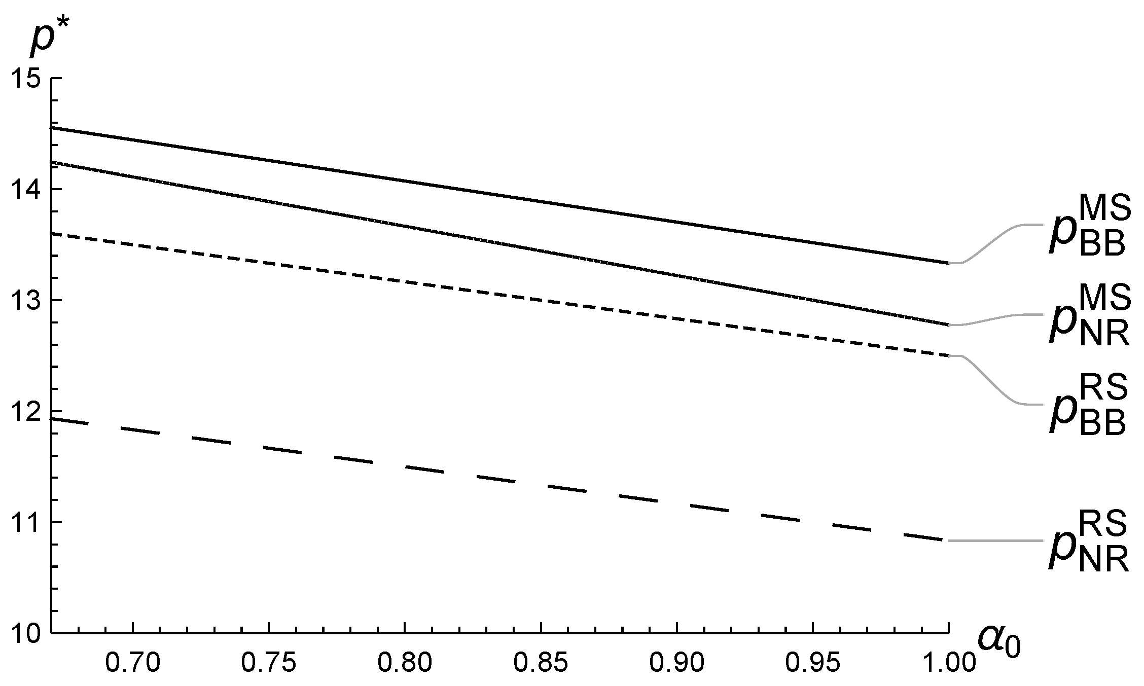
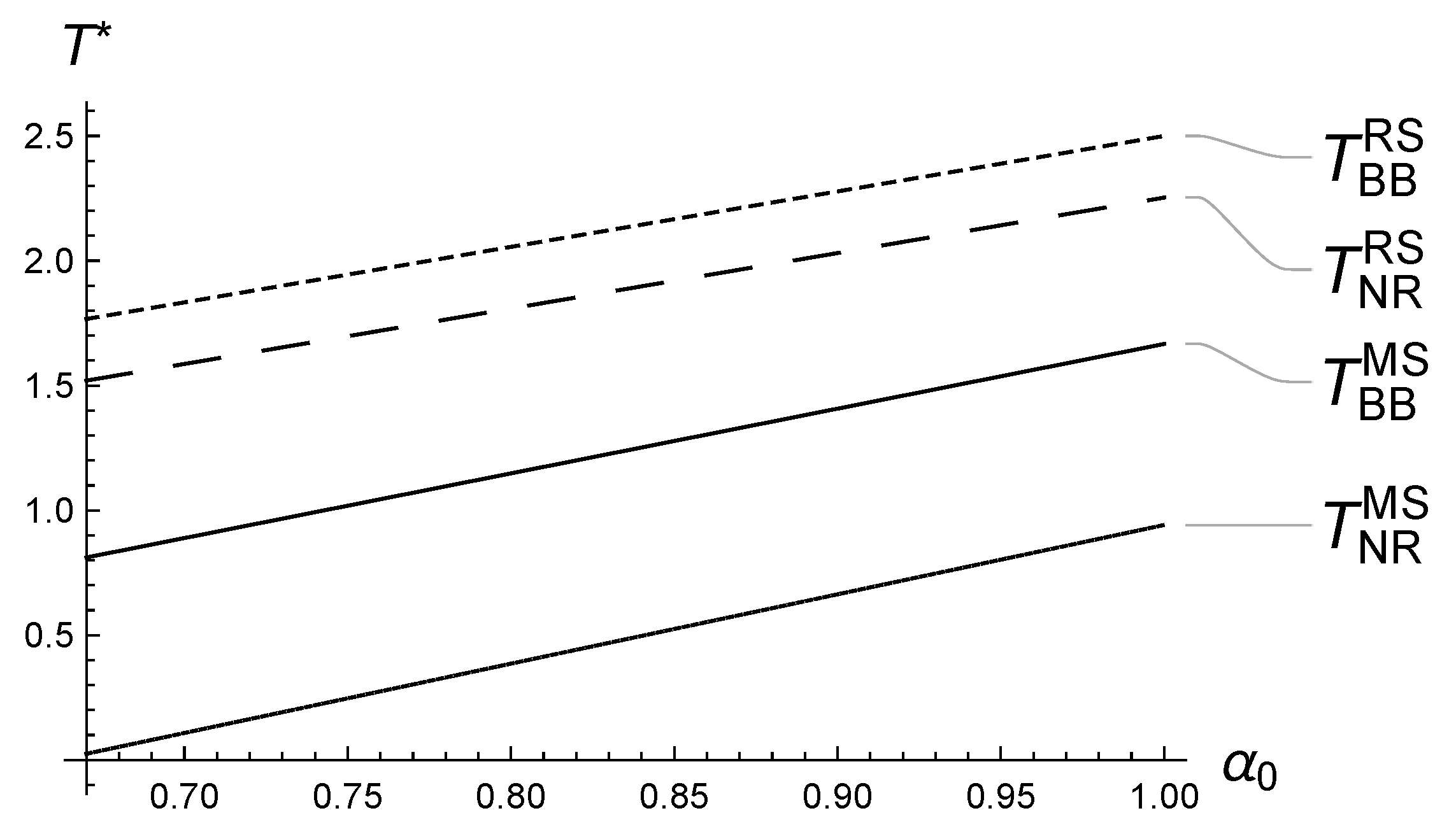
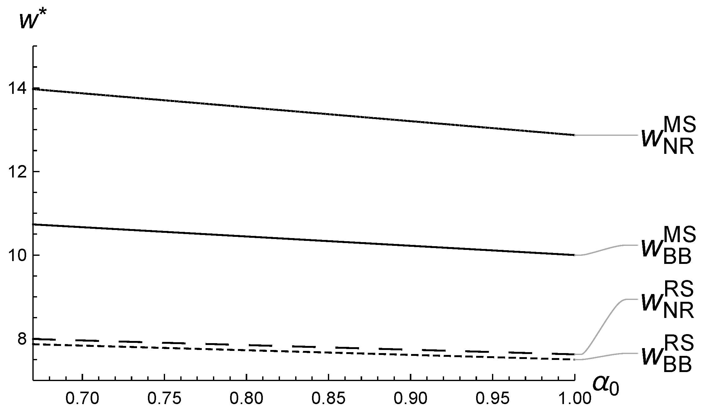
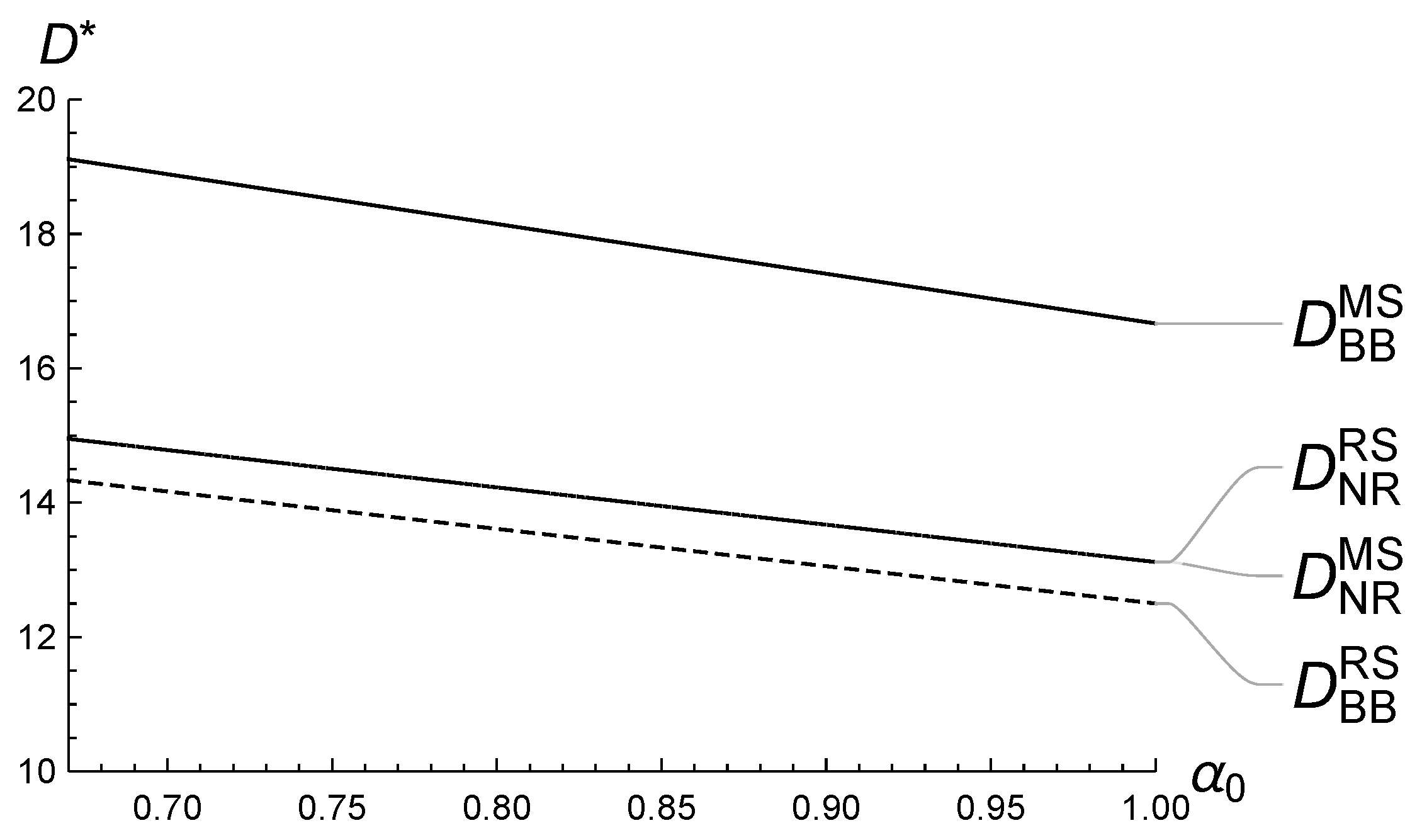
To investigate the impact of the maximum return rate α 0 on the equilibrium and compare the results under different handling strategies and also different power structures, let α 0 varies and β 0 = 0.3 , η = 0.1 , 1 without any lose of generality. The results are shown in Figure 2, Figure 3, Figure 4, Figure 5, Figure 6 and Figure 7.
Figure 2 describes the relationship between the equilibrium price and the maximum return rate α 0 when the e-tailer adopts different reverse channel strategies in the supply chain of MS and RS. As shown in the figure, the equilibrium prices in different supply chain structures and different return channels all decrease in the maximum return rate. This means that if the maximum return rate increases, the e-tailer will certainly reduce the price, which is not affected by the supply chain structure and other factors. At the same time, it can be seen from the figure that the equilibrium price of the e-tailer in the MS supply chain must be higher than that in the RS supply chain, no matter what the handling strategy is, that is p BB M S > p BB R S and p NR M S > p NR R S .
It is worth noting that, the relationship between the equilibrium price under different handling strategy in each supply chain depends on η . When η = 0.1 > 0 , there are p NR M S > p BB M S and p NR R S > p BB R S . It means that when returns have higher residual value, salvaging returns by e-tailers can achieve higher prices. The difference is that the threshold is 0 in the RS supply chain, while the threshold is related to other parameters such as return parameters in the MS supply chain. Figure 3 shows the reverse situation when η = 1 .
As shown in Figure 3, when η = 1 , the relationship between the equilibrium price of different reverse channels in the MS (RS) supply chain is opposite to that described in Figure 2. When η is small, p NR M S < p BB M S and p NR R S < p BB R S . Note that the effect of α 0 on the equilibrium price in the four cases remains unchanged. The equilibrium prices of the two reverse channels of the MS supply chain are still higher than their corresponding prices in the RS supply chain.
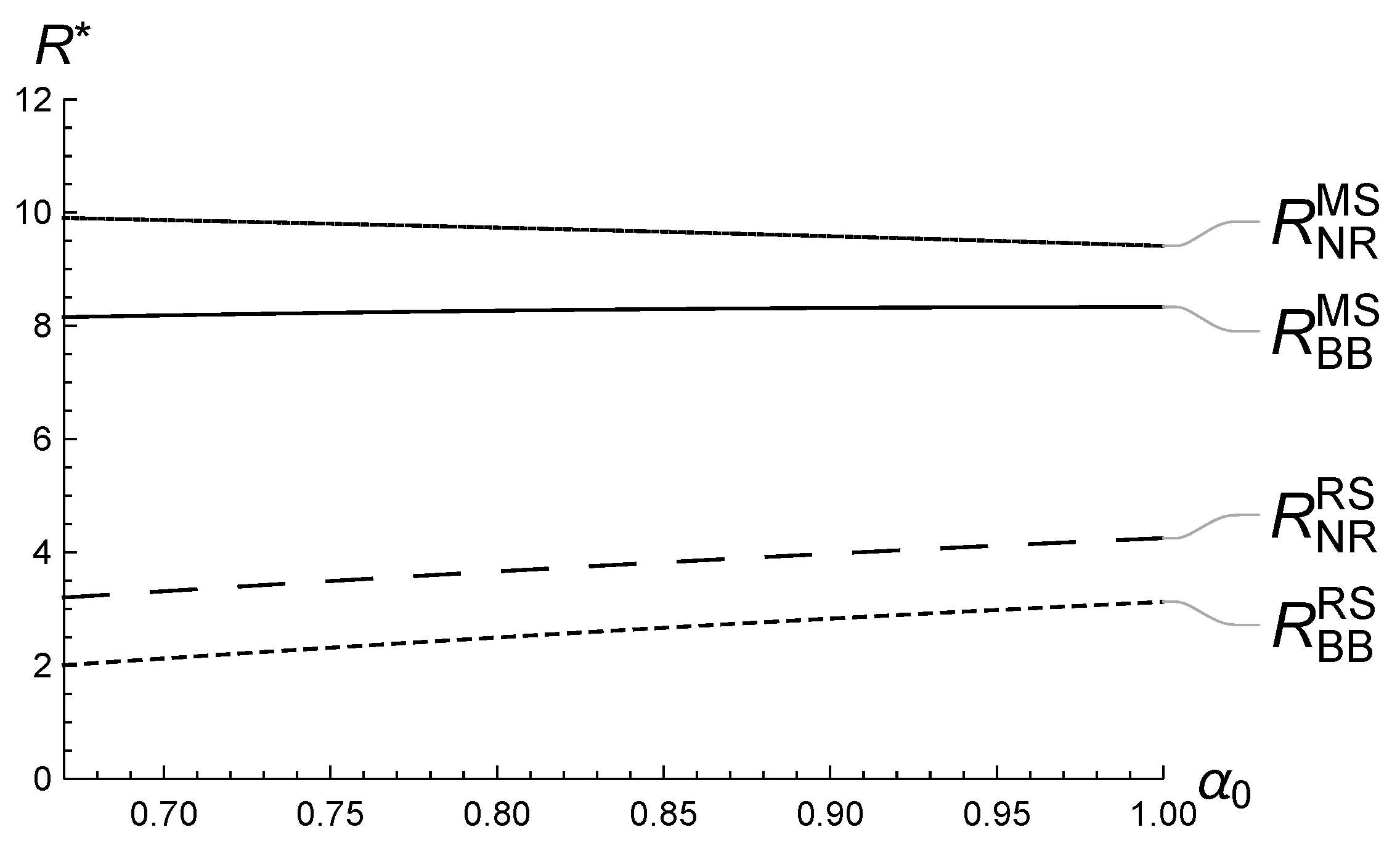
Figure 4, Figure 5, Figure 6 and Figure 7 show the impact of the maximum return rate α 0 on the equilibrium PDL of the e-tailer, the equilibrium wholesale price of the manufacturer, the equilibrium demand and returns, respectively. As shown in the figure, if the maximum return rate increases, then the e-tailer will extend PDL, the manufacturer will reduce the wholesale price, and at the same time, the demand in the supply chain will decrease and the return will increase. Additionally, we have T BB M S < T BB R S , T NR M S < p NR R S , w BB M S > w BB R S and w NR M S > w NR R S . Moreover, it can be proved that when the e-tailer takes the responsibility to salvage returns, the demands under the MS and RS supply chain are equal, namely D NR M S = D NR M S . Note that the above result is robust with any parameters.

5.2. Numerical Analysis of β 0 ’s Impact on the Equilibrium

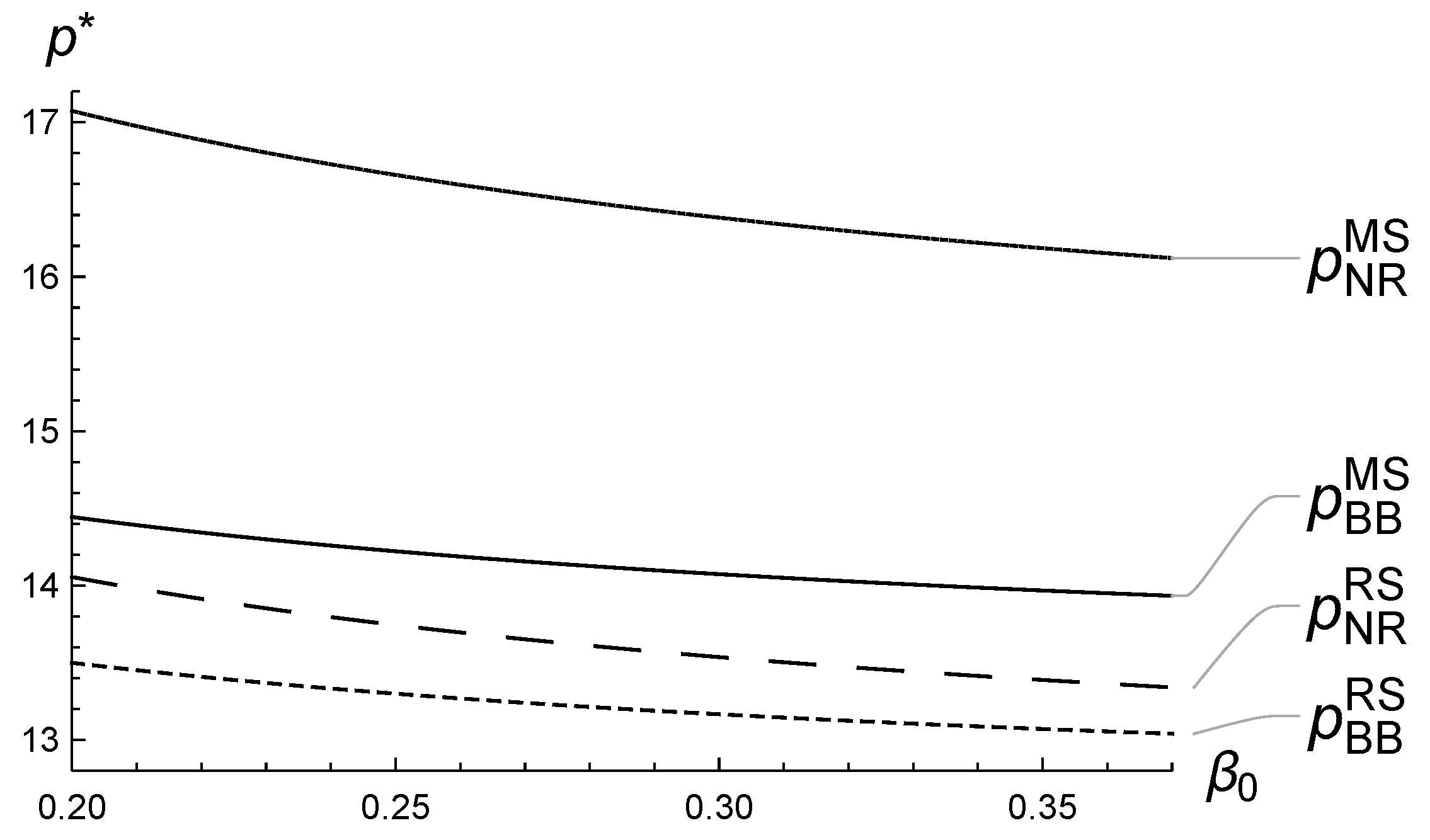
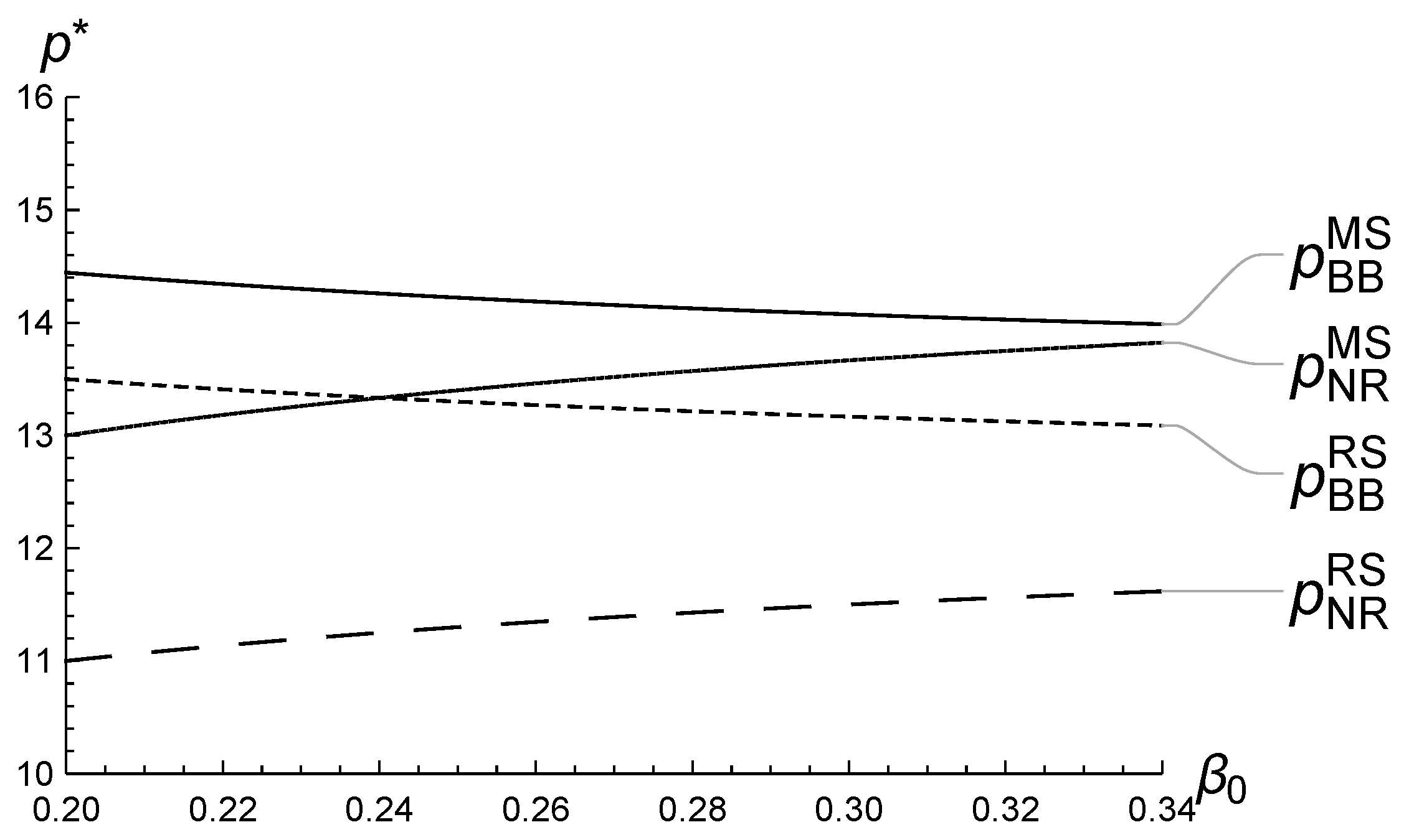
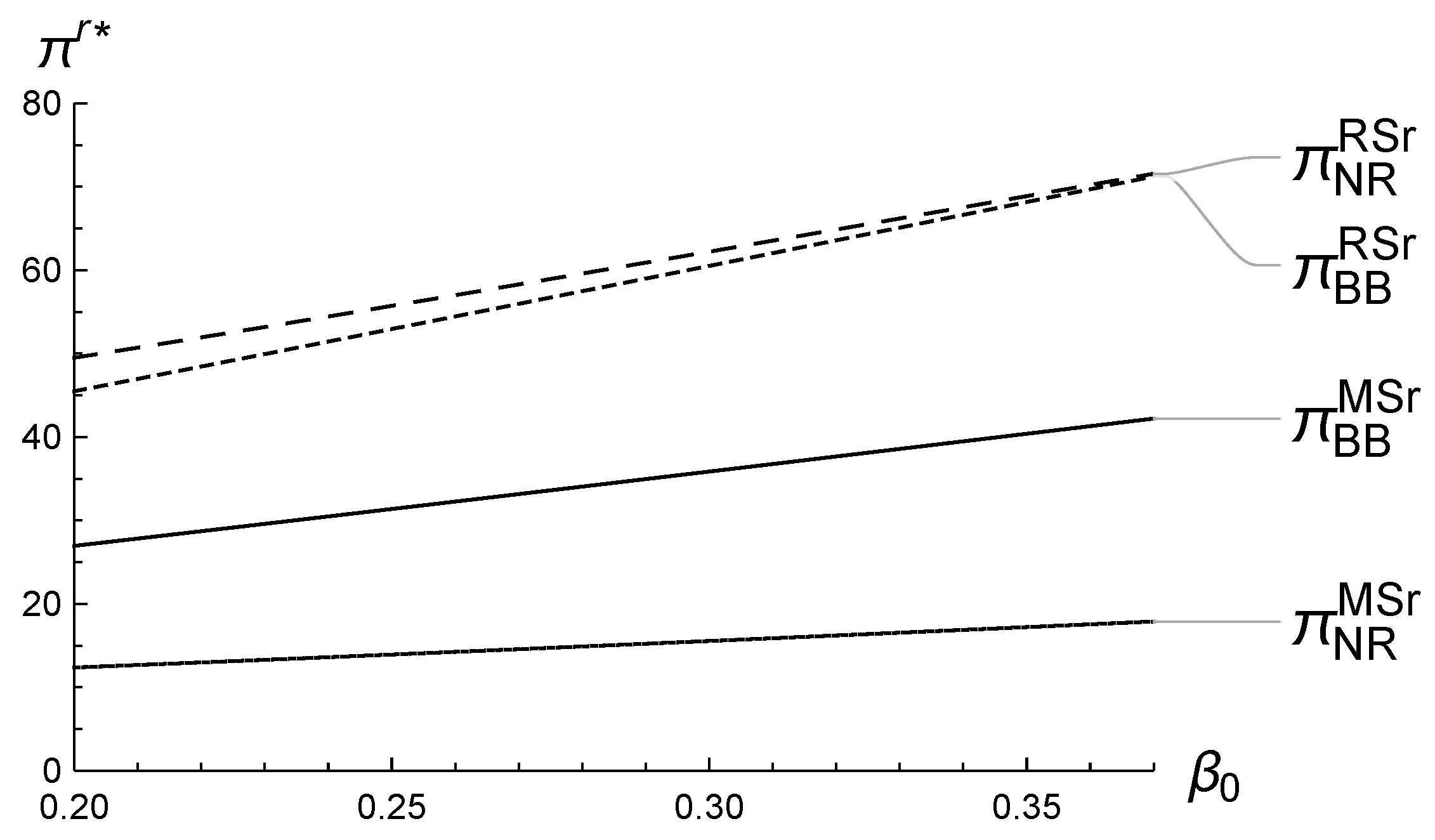
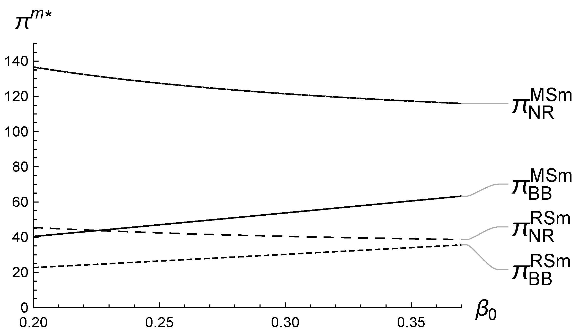
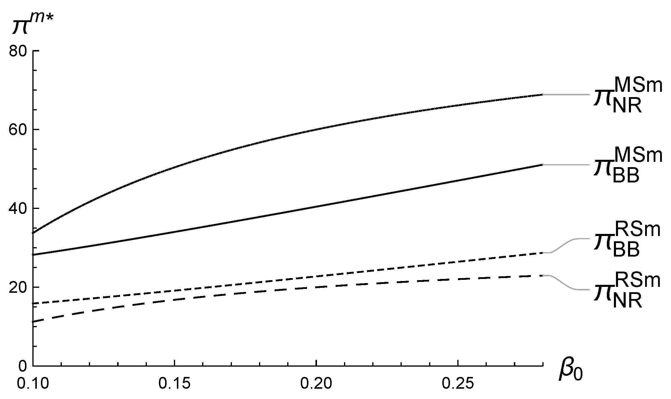
In this subsection, we will discuss the return rate sensitivity to PDL β 0 on the equilibrium, which summarized in Figure 8, Figure 9 and Figure 10. According to Corollary 2, when the return policy is NR , the effect of β 0 on the supply chain equilibrium decision depends on the relationship between α 0 and η , which is divided into two cases. Therefore, this subsection assumes that α 0 = 0.8 and discusses the effect of β 0 on the equilibrium price when η equals 0.1 or 1 , as shown in Figure 8 and Figure 9. In the meantime, from Corollarys 3 and 4, it can be seen that the equilibrium profit of the e-tailer monotonically increases in β 0 (see Figure 10), and the manufacturer’s equilibrium profit is non-monotonic (see Figure 11 and Figure 12).
As shown in Figure 8 and Figure 9, the equilibrium price always decreases in β 0 when the reverse channel is  BB  in both MS and RS supply chains. However, the relationship between p NR and β 0 is non-monotonic and dependent on two other parameters. Specifically, when η = 0.1 , it satisfies that η > 1 1 α 0 = 0.2 , and thus it can be inferred from Corollary 2 that p NR M S also decreases in β 0 . When η gets smaller, for example, η = 1 , p NR M S starts increasing in β 0 since η < 1 1 α 0 . Note that the impacts of β 0 on the equilibrium PDL and the wholesale price are also non-monotonic under  NR  strategy and the impacts of β 0 on the equilibrium solutions are identical under different power structures. In addition, by comparing Figure 8 and Figure 9, it can be verified that the equilibrium price in the MS supply chain is higher than that in the RS supply chain when the same reverse channel is adopted.
Though the impacts of β 0 on the equilibrium price and PDL depend on α 0 and η , the profit of the e-tailer will monotonically increase in β 0 (see Figure 10). In our model, a greater value of β 0 signifies that consumer return behavior is more sensitive to the promised delivery time. More importantly, it also means that the e-tailer’s ability of reducing returns through a longer PDL becomes stronger as β 0 increases. As a result, the e-tailer’s profit always increases in β 0 regardless of the structure of the supply chain and the reverse channel. By contrast, the manufacturer’s profit may be lost due to the increase of β 0 (see Figure 11 and Figure 12).
As shown in Figure 11 and Figure 12, both π BB M S m and π BB R S m increase in β 0 . However, when the reverse channel is  NR  , the manufacturer’s profit decreases in β 0 when η is relatively large. The possible reason is that the e-tailer will reduce price and prolong PDL as β 0 increases when η is relatively large, which leads to less demand but more net sales ( D NR R NR ) since product returns are well-controlled. Therefore, for manufacturers, less demands and lower wholesale price will inevitably lead to loss of profits. In addition, it can be found that the profits of manufacturers in the MS supply chain are always higher than these of the RS supply chain, while the e-tailers’ profits are opposite.

5.3. Numerical Analysis of η ’s Impact on the Equilibrium

In this subsection, numerical analysis is conducted to explore the impact of the reselling ratio η on the equilibrium decisions and handling strategies under different supply chain power structure. Similarly, let other parameters be fixed, such as α 0 = 0.8 and β 0 = 0.25 .
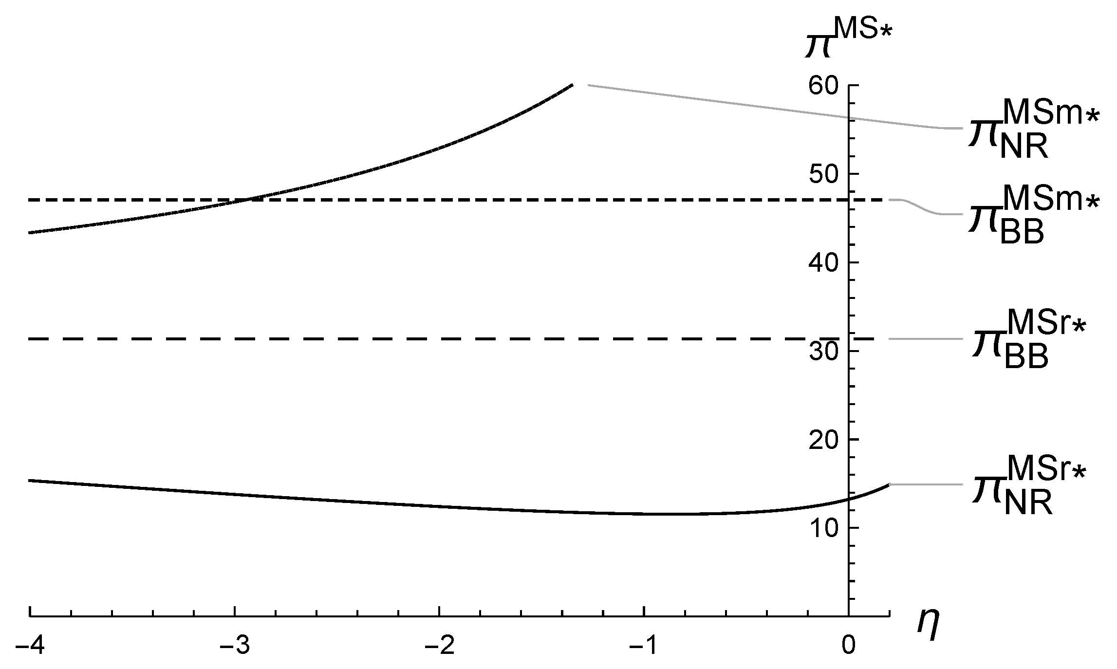
Figure 13 describes how the profits of the manufacturer and the e-tailer change with η in the MS supply chain. Note that all the profits under  BB  strategy are independent of η , and thus they all appear as a straight line parallel to the η axis. It can be found that π BB M S r > π NR M S r always holds. That is to say, the e-tailer always prefers to return the units to the manufacturer. In the meantime, the line of π BB M S m and π NR M S m intersect at one point, namely η ^ . When η η ^ , the manufacturer receives higher profit by choosing  BB  strategy, and  NR  strategy is preferred otherwise. As mentioned earlier, in the MS supply chain, the manufacturer first decides the handling strategy, and thus this intersection is the threshold of the reverse channel selection. Since the e-tailer always chooses BB strategy, from the situation after the intersection, the optimal reverse channel of the e-tailer is not consistent with the manufacturer, and the profit is lost.
It is worth noting that the relationship between π NR M S r and η is non-monotonic. The profit of the e-tailer under  NR  strategy does not necessarily increase in the market discount, η , that is, the value the e-tailer obtained from salvaging returns. When η is less than a certain value, the more value the returned unit is, the less profit of the manufacturer will be (see Corollary 3). This is because the e-tailer tends to increase the profit margin and the demand when the reselling ratio increases. However, the number of product returns increases as well, and the e-tailer will benefit from it unless η is relatively large.
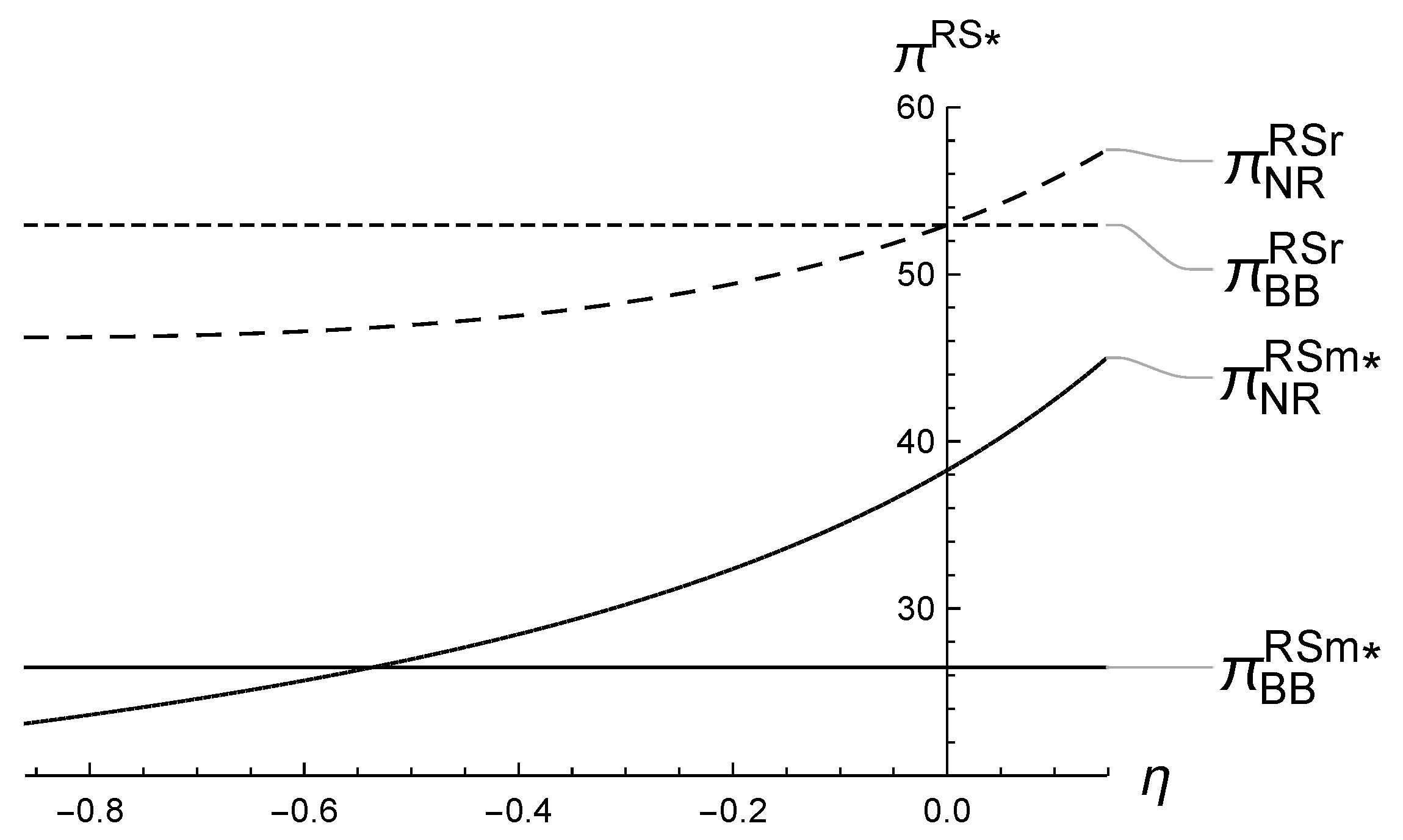
Figure 14 demonstrates the impact of the reselling ratio, η , on the profits of the manufacturer and the e-tailer under each handling strategy in the RS supply chain, respectively. This study finds that the reselling ratio threshold that determines the reverse channel is a constant value, 0. Therefore, the line of π BB R S r and π NR R S r interact at η = 0 in the figure. This result is intuitive that the e-tailer will directly handle product returns in the secondary market if the reselling ratio is positive, and take back to the manufacturer otherwise, since the e-tailer has more power in the decentralized supply chain. Compared to the e-tailer, the manufacturer’s handling strategy depends on several parameters as in the MS case. As can be seen from the figure, when η is between about −0.6 and 0, since the reverse channel is determined by the e-tailer, which is the BB strategy, the manufacturer’s profit will be lost.
In summary, by comparing the impact of the return-related parameters on the decentralized supply chain decision and profit under different supply chain power structures, the following observations can be summarized:
Observation 1. 
The impacts of return-related parameters, α 0 , β 0 and η, on the manufacturer’s profit are identical between different supply chain power structures. The manufacturer’ profit may be lost if products returns are more sensitive to PDL, but it always benefits the e-tailer.
Observation 2. 
Under the   NR   strategy, the impacts of the reselling ratio, η, on the equilibrium profit of the e-tailer are different in the MS and RS supply chain. A larger reselling ratio for the e-tailer may counterintuitively lead to lower profits.
Observation 3. 
It is the threshold of η that affects the handling strategy in both MS and RS supply chains. However, the threshold of η depends on the returns parameters (i.e., α 0 and β 0 ) in the MS model, and equals to the critical value, 0, in the RS supply chain.
Observation 4. 
Under both  BB   and   NR   strategies, the relationships between the equilibrium decisions and profits in the MS and RS supply chain are: (1) p M S > p R S , T M S > T R S , w M S > w R S ; (2) π M S r > π R S r , π M S m > π R S m .

6. Discussion and Managerial Implications

A central finding of our paper is that the supply chain’s power structure is not just a determinant of profit distribution but a fundamental architect of the reverse channel’s operational design. In a retailer-led (RS) supply chain, the decision is intuitive: the powerful e-tailer like Walmart or Amazon will handle returns itself if it can extract positive value from them. However, in a manufacturer-led (MS) supply chain, the logic is distorted by the classic “double marginalization” problem. Our model shows that a less powerful e-tailer (e.g., an independent boutique selling products from a dominant brand like Nike) consistently prefers the manufacturer to buy back returns, even when it is highly efficient at reselling them. This is because a dominant manufacturer, anticipating the e-tailer’s potential profit from returns, will strategically increase the wholesale price to capture those gains, leaving the e-tailer with a smaller margin. This theoretical distinction translates into clear strategic guidance: the choice between investing in in-house reverse logistics versus negotiating a manufacturer buy-back program is critically contingent on the e-tailer’s power position. For less powerful e-tailers, such as small businesses selling powerful national brands, the primary focus should be on negotiating favorable buy-back terms, as heavy investment in internal reverse logistics may not yield higher profits. In contrast, for powerful e-tailers like large online marketplaces, investments in improving reverse logistics efficiency will directly translate to higher profitability.
Our model also uncovers a paradoxical effect in the MS scenario, where an e-tailer’s increasing efficiency in handling returns can, under certain conditions, lead to lower profits. This non-monotonic relationship highlights a complex trade-off between forward-channel sales incentives and reverse-channel costs. This theoretical finding has a strong parallel in the practical phenomenon of “bracketing” where consumers intentionally order multiple product variations with the plan to return most of them. Our model provides a strategic explanation: when an e-tailer becomes very efficient at reselling, the dominant manufacturer may set a wholesale price that encourages the e-tailer to adopt marketing strategies (e.g., “free returns, try at home”—a model famously perfected by Zappos) that inadvertently encourage bracketing. The resulting surge in return volume and associated operational costs can ultimately overwhelm the profit gained from each resold item. This insight leads to a crucial managerial takeaway: e-tailers must be wary of a myopic focus on maximizing the salvage value of each returned item. The optimal strategy requires a holistic view that balances the efficiency of the reverse channel with its impact on forward-channel demand and consumer behavior. For e-tailers in manufacturer-dominated channels, a high reselling ratio may not translate to higher profits if it incentivizes the manufacturer to increase wholesale prices commensurately.
Finally, our model explicitly links the operational Promised Delivery Lead Time (PDL) decision to the return rate, offering a framework for managers to think about these choices jointly. A shorter PDL is a powerful marketing tool but directly increases the operational risk of service-level returns. Therefore, the PDL should be viewed as a dual-impact lever, requiring managers to forecast its effect not only on sales but also on the expected volume and cost of returns. For manufacturers, this implies that a one-size-fits-all return policy is suboptimal. The decision to offer a buy-back program, as seen in the complex vendor agreements of electronics retailers like Best Buy, should be viewed as a strategic instrument for channel coordination. By absorbing the return risk from less efficient retail partners, a manufacturer can incentivize them to adopt pricing and PDL strategies more beneficial for the supply chain as a whole. For e-tailers, the optimal PDL becomes contingent on the returns handling strategy. If a favorable buy-back agreement is in place, the e-tailer is insulated from return costs and can more aggressively use a short PDL to drive sales. Conversely, if the e-tailer is responsible for returns, it may need to quote a more conservative (longer) PDL to mitigate the risk of being inundated with costly returns, especially if its reselling efficiency is low.

7. Conclusions

In an increasingly competitive e-commerce landscape, the management of product returns has evolved from a purely logistical issue into a critical strategic challenge. This paper addresses the pressing problem of service-level returns—those driven by operational failures like unfulfilled delivery promises. Our central contribution is the development of an integrated game-theoretic framework that theoretically links a forward-channel operational decision (the PDL) to the endogenous rate of returns and the subsequent strategic choice of the reverse-channel structure. By analyzing these dynamics under different supply chain power structures, we provide a more holistic understanding of the interplay between delivery promises, pricing, and returns handling strategy. Our analysis demonstrates that the optimal reverse channel structure is governed by the e-tailer’s efficiency in recovering value from returns, but this relationship is fundamentally contingent on the supply chain’s power structure. In a manufacturer-led chain, power dynamics can lead to counterintuitive outcomes where the e-tailer prefers a buy-back policy even when it is efficient at reselling. In contrast, a retailer-led chain follows a more intuitive, profit-driven logic. These findings underscore that channel power is not just a determinant of profit distribution but a fundamental shaper of the supply chain’s operational architecture.
Several directions can serve as future efforts. First, our model utilizes linear demand and return functions for analytical tractability. Future work could explore non-linear relationships to test the robustness of our findings. Second, our analysis is focused on a single manufacturer and e-tailer. Extending the model to a competitive setting with multiple e-tailers would introduce horizontal dynamics and could yield further insights into how competition shapes returns handling strategies. Third, our model assumes a standard full-refund policy. However, practices like “returnless refunds” and the use of return-freight insurance are becoming more common. Investigating how these novel policies interact with PDL decisions and the choice of handling strategy would be a valuable extension. Furthermore, the rise of technologies like Augmented Reality (AR) to reduce product mismatch and AI to forecast returns is changing the landscape. Future models could examine how investments in such “transparency initiatives” alter the parameters of our model and influence strategic choices. Finally, our findings are based on a theoretical model and have not been empirically validated. Empirically testing the model’s propositions using real-world data from e-commerce platforms would be a significant step toward confirming its managerial relevance.

Funding

This work was supported by Guangdong Basic and Applied Basic Research Foundation [2021A1515110193], Ministry of Education Humanities and Social Sciences Research Project [22YJC630215].

Institutional Review Board Statement

Not applicable.

Informed Consent Statement

Not applicable.

Data Availability Statement

Data sharing is not applicable to this article as no new data were created or analyzed in this study.

Conflicts of Interest

The author declares no conflicts of interest.

Appendix A. Postponed Proofs

Appendix A.1. Proof of Proposition 1

Proof. 
By solving the first order conditions of the objective function in (3), we obtain four solutions:
  • p = d 0 β 0 + s 2 ( 1 α 0 ) 3 s 1 β 0 + 2 w 3 , T = d 0 s 1 w 3 s 2 2 ( 1 α 0 ) 3 β 0 ;
  • p = w , T = d 0 s 1 w s 2 ;
  • p = β 0 d 0 + 1 α 0 s 2 β 0 s 1 , T = α 0 1 β 0 ;
  • p = w , T = α 0 1 β 0 .
The profit value at each above solutions is: π i = β 0 d 0 w s 1 α 0 s 2 + s 2 3 27 s 1 s 2 β 0 2 ( > 0 ) , π ii = 0 , π iii = 0 and π iv = 0 , respectively. Therefore, solutions ii, iii, and iv are ruled out. We then verify that solution i is the global maximum.
We compute the second order partials of (3),
2 π BB r p 2 = 2 s 1 α 0 β 0 T 1 , 2 π BB r p T = β 0 d 0 + s 1 ( w 2 p ) + s 2 α 0 2 β 0 T 1 , 2 π BB r T p = β 0 d 0 + s 1 ( w 2 p ) + s 2 α 0 2 β 0 T 1 , 2 π BB r T 2 = 2 β 0 s 2 ( w p ) ,
and obtain the Hessian H = 2 π BB r p 2 2 π BB r p T 2 π BB r T p 2 π BB r T 2 . The second principle minor at solution i is D = 1 3 β 0 d 0 + α 0 1 s 2 + β 0 s 1 w 2 > 0 . Since lim p ± π BB r = and lim T ± π BB r = , the local maximum (solution i) is the global maximum (best response).
Substituting the best response function of the e-tailer into the profit function of the manufacturer (4) gives the single-variable optimization problem with respect to w:
max w π BB m = 1 9 s 2 β 0 ( w c ) ( d 0 β 0 + s 2 ( 1 α 0 ) s 1 β 0 w ) 2 .
Similarly, by solving the first order condition of the objective function, we obtain two solutions: β 0 d 0 + 1 α 0 s 2 β 0 s 1 and 2 β 0 c s 1 + β 0 d 0 + 1 α 0 s 2 3 β 0 s 1 . The profit value at each above solutions is: 0 and 4 β 0 d 0 c s 1 + 1 α 0 s 2 3 243 β 0 2 s 1 s 2 . Since d 0 s 1 c s 2 α 0 β 0 > 0 as assumed previously, 4 β 0 d 0 c s 1 + 1 α 0 s 2 3 243 β 0 2 s 1 s 2 > 0 . We then verify that w = 2 β 0 c s 1 + β 0 d 0 + 1 α 0 s 2 3 β 0 s 1 is the global maximum.
The second order condition satisfies 2 π BB m w 2 = 2 s 1 β 0 c s 1 β 0 d 0 + α 0 1 s 2 9 s 2 < 0 , since d 0 s 1 w s 2 α 0 β 0 > 0 , namely w < β 0 d 0 s 2 α 0 s 1 β 0 < β 0 d 0 + 1 α 0 s 2 β 0 s 1 . Note that π BB m ( w = c ) = 0 and π BB m ( w = β 0 d 0 + 1 α 0 s 2 β 0 s 1 ) = 0 , thus this critical point is global maximum. □

Appendix A.2. Proof of Proposition 2

Proof. 
By solving the first order conditions of the objective function in (6), we obtain four solutions:
  • p = β 0 ( η 1 ) d 0 + 2 s 1 w + s 2 α 0 ( η ) + α 0 1 3 β 0 ( η 1 ) s 1 , T = 1 3 2 α + 1 η 1 β + d 0 s 1 w s 2 ;
  • p = w , T = d 0 s 1 w s 2 ;
  • p = d 0 + s 2 α 0 ( η 1 ) + 1 β 0 ( 1 η ) s 1 , T = α 0 + 1 η 1 β 0 ;
  • p = w , T = α 0 + 1 η 1 β 0 .
The profit value at each above solutions is π i = β 0 ( η 1 ) d 0 s 1 w + α 0 ( η 1 ) s 2 + s 2 3 27 β 0 2 ( η 1 ) 2 s 1 s 2 ( > 0 ) ,   π ii = 0 , π iii = 0 and π iv = 0 , respectively. Therefore, solutions ii, iii, and iv are ruled out. We then verify that solution i is the global maximum.
We compute the second order partials of (6),
2 π NR r p 2 = 2 s 1 α 0 ( η 1 ) + T β 0 β 0 η + 1 , 2 π NR r p T = s 2 α 0 ( η ) + α 0 + 2 β 0 ( η 1 ) T 1 β 0 ( η 1 ) d 0 + s 1 ( w 2 p ) , 2 π NR r T p = s 2 α 0 ( η ) + α 0 + 2 β 0 ( η 1 ) T 1 β 0 ( η 1 ) d 0 + s 1 ( w 2 p ) , 2 π NR r T 2 = 2 β 0 ( η 1 ) s 2 ( p w ) ,
and obtain the Hessian H = 2 π NR r p 2 2 π NR r p T 2 π NR r T p 2 π NR r T 2 . The second principle minor at solution i is D = 1 3 β 0 ( η 1 ) d 0 s 1 w + α 0 ( η 1 ) s 2 + s 2 2 > 0 . Since lim p ± π NR r = and lim T ± π NR r = , the local maximum (solution i) is the global maximum (best response).
Substituting the best response function of the e-tailer into the profit function of the manufacturer (7) gives the single-variable optimization problem with respect to w:
max w π NR m = ( w c ) ( s 2 s 2 α 0 ( 1 η ) + ( d 0 s 1 w ) β 0 ( 1 η ) ) 3 β 0 ( 1 η ) .
It is easy to verify that 2 π NR m w 2 = 2 s 1 3 < 0 . Therefore, the only critical point
w = d 0 β 0 ( 1 η ) + s 2 ( 1 α 0 ( 1 η ) ) 2 s 1 β 0 ( 1 η ) + c 2 ,
is global maximum. Substituting w into the best response functions of the e-tailer p ( w ) and T ( w ) gives the result in Proposition 2.

Appendix A.3. Proof of Proposition 3

Proof. 
From Equations (9) and (11), we obtain that π BB , MS , m π NR , MS , m = 16 β 0 d 0 c s 1 + 1 α 0 s 2 3 81 s 2 β 0 d 0 c s 1 α 0 s 2 + s 2 1 η 2 . It is easy to verify that π BB , MS , m π NR , MS , m = 1 if η = η ^ . Recalling that we assume d 0 s 1 c + s 2 α 0 β 0 to ensure the positiveness of the demand, the result in Proposition 3 is then obtained. □

Appendix A.4. Proof of Corollary 8

Proof. 
It is easy to prove that π NR R S m > π BB R S m if
η > η ˜ = 3 s 2 β 0 d 0 c s 1 + 1 α 0 s 2 3 / 2 + α 0 s 2 β 0 d 0 c s 1 3 s 2 3 α 0 s 2 β 0 d 0 c s 1 3 3 β 0 s 2 2 d 0 c s 1 + 3 α 0 s 2 3 s 2 3 .
Thus, the manufacturer prefers NR strategy. If η η ˜ , then π NR R S m π BB R S m . □

References

  1. Tapia, J.; Fariña, P.; Urbina, I.; Dujovne, D. Examining the retail delivery choice behavior in a technology-aware market. J. Theor. Appl. Electron. Commer. Res. 2024, 19, 1392–1410. [Google Scholar] [CrossRef]
  2. Niu, B.; Liu, J.; Zhang, J.; Chen, K. Promised-delivery-time-driven reselling facing global platform’s private label competition: Game analysis and data validation. Omega 2024, 123, 102990. [Google Scholar] [CrossRef]
  3. Hu, L.; Zhou, X.; Choi, T.M.; Du, S. Making Delivery Platform Drivers Safer: Platform Responsibility Versus Consumer Empowerment. Prod. Oper. Manag. 2025, 34, 2104–2123. [Google Scholar] [CrossRef]
  4. Chung, W.; Talluri, S.; Kovács, G. Investigating the effects of lead-time uncertainties and safety stocks on logistical performance in a border-crossing JIT supply chain. Comput. Ind. Eng. 2018, 118, 440–450. [Google Scholar] [CrossRef]
  5. Rao, S.; Rabinovich, E.; Raju, D. The role of physical distribution services as determinants of product returns in Internet retailing. J. Oper. Manag. 2014, 32, 295–312. [Google Scholar] [CrossRef]
  6. Cui, R.; Lu, Z.; Sun, T.; Golden, J.M. Sooner or later? Promising delivery speed in online retail. Manuf. Serv. Oper. Manag. 2024, 26, 233–251. [Google Scholar] [CrossRef]
  7. Li, Z.; Chen, X.; Li, S. Delivery timeliness disclosure strategy in platform-based instant retail industries: Understanding the effect of consumer loss aversion. Transp. Res. Part E Logist. Transp. Rev. 2025, 201, 104288. [Google Scholar] [CrossRef]
  8. Shulman, J.D.; Coughlan, A.T.; Savaskan, R.C. Optimal reverse channel structure for consumer product returns. Mark. Sci. 2010, 29, 1071–1085. [Google Scholar] [CrossRef]
  9. Chen, J.; Chen, B. Competing with customer returns policies. Int. J. Prod. Res. 2016, 54, 2093–2107. [Google Scholar] [CrossRef]
  10. Yi, L. Research on B2C cross-border electronic commerce return logistics model selection based on estimated return rate. J. Theor. Appl. Electron. Commer. Res. 2024, 19, 1034–1059. [Google Scholar]
  11. Altug, M.S.; Aydinliyim, T.; Jain, A. Managing opportunistic consumer returns in retail operations. Manag. Sci. 2021, 67, 5660–5678. [Google Scholar] [CrossRef]
  12. Pekgün, P.; Griffin, P.M.; Keskinocak, P. Centralized versus decentralized competition for price and lead-time sensitive demand. Decis. Sci. 2017, 48, 1198–1227. [Google Scholar] [CrossRef]
  13. Zhang, Y.; Yu, P.; Feng, T. Full Quantity or Full Credit? Choosing the Right Buyback Policy for a Behavioral Retailer. Manuf. Serv. Oper. Manag. 2024, 26, 2212–2230. [Google Scholar] [CrossRef]
  14. Crocker, K.J.; Letizia, P. Optimal policies for recovering the value of consumer returns. Prod. Oper. Manag. 2014, 23, 1667–1680. [Google Scholar] [CrossRef]
  15. Frei, R.; Jack, L.; Brown, S. Product returns: A growing problem for business, society and environment. Int. J. Oper. Prod. Manag. 2020, 40, 1613–1621. [Google Scholar] [CrossRef]
  16. Yang, L.; Li, X.; Xia, Y.; Aneja, Y. Returns operations in omnichannel retailing with buy-online-and-return-to-store. Omega 2023, 119, 102874. [Google Scholar] [CrossRef]
  17. Huang, X.; Gu, J.W.; Ching, W.K.; Siu, T.K. Impact of secondary market on consumer return policies and supply chain coordination. Omega 2014, 45, 57–70. [Google Scholar] [CrossRef]
  18. Wei, J.; Zhao, J.; Li, Y. Pricing decisions for complementary products with firms’ different market powers. Eur. J. Oper. Res. 2013, 224, 507–519. [Google Scholar] [CrossRef]
  19. El-Ansary, A.I.; Stern, L.W. Power measurement in the distribution channel. J. Mark. Res. 1972, 9, 47–52. [Google Scholar] [CrossRef]
  20. Pan, K.; Lai, K.K.; Leung, S.C.; Xiao, D. Revenue-sharing versus wholesale price mechanisms under different channel power structures. Eur. J. Oper. Res. 2010, 203, 532–538. [Google Scholar] [CrossRef]
  21. So, K.C.; Song, J.S. Price, delivery time guarantees and capacity selection. Eur. J. Oper. Res. 1998, 111, 28–49. [Google Scholar] [CrossRef]
  22. Li, Y.; Lin, Q.; Ye, F. Pricing and promised delivery lead time decisions with a risk-averse agent. Int. J. Prod. Res. 2014, 52, 3518–3537. [Google Scholar] [CrossRef]
  23. Albana, A.S.; Frein, Y.; Hammami, R. Effect of a lead time-dependent cost on lead time quotation, pricing, and capacity decisions in a stochastic make-to-order system with endogenous demand. Int. J. Prod. Econ. 2018, 203, 83–95. [Google Scholar] [CrossRef]
  24. Zhai, Y.; Cheng, T. Lead-time quotation and hedging coordination in make-to-order supply chain. Eur. J. Oper. Res. 2022, 300, 449–460. [Google Scholar] [CrossRef]
  25. Zhai, Y.; Hua, G.; Cheng, M.; Cheng, T. Production lead-time hedging and order allocation in an MTO supply chain. Eur. J. Oper. Res. 2023, 311, 887–905. [Google Scholar] [CrossRef]
  26. Yang, Z.; Zheng, Y.; Li, J.; Zhu, S.X.; Yang, C. Delivery service for a service-oriented manufacturing supply chain with procurement and delivery time decisions. Int. J. Prod. Res. 2024, 62, 7581–7597. [Google Scholar] [CrossRef]
  27. So, K.C. Price and Time Competition for Service Delivery. Manuf. Serv. Oper. Manag. 2000, 2, 392–409. [Google Scholar] [CrossRef]
  28. Niu, B.; Dai, Z.; Zhuo, X. Co-opetition effect of promised-delivery-time sensitive demand on air cargo carriers’ big data investment and demand signal sharing decisions. Transp. Res. Part E Logist. Transp. Rev. 2019, 123, 29–44. [Google Scholar] [CrossRef]
  29. Ye, F.; Xie, Z.; Tong, Y.; Li, Y. Promised delivery time: Implications for retailer’s optimal sales channel strategy. Comput. Ind. Eng. 2020, 144, 106474. [Google Scholar] [CrossRef]
  30. Gong, C.; Song, H.; Chen, D.; Day, S.J.; Ignatius, J. Logistics sourcing of e-commerce firms considering promised delivery time and environmental sustainability. Eur. J. Oper. Res. 2024, 317, 60–75. [Google Scholar] [CrossRef]
  31. Zhao, S.; Wu, F.; Jia, T.; Shu, L. The impact of product returns on price and delivery time competition in online retailing. Comput. Ind. Eng. 2018, 125, 658–667. [Google Scholar] [CrossRef]
  32. Ahmed, A.; Deokar, A.; Lee, H.C.B.; Summerfield, N. The role of commitment in online reputation systems: An empirical study of express delivery promise in an E-commerce platform. Decis. Support Syst. 2024, 176, 114061. [Google Scholar] [CrossRef]
  33. Wagner, L.; Calvo, E.; Amorim, P. Better Together! The Consumer Implications of Delivery Consolidation. Manuf. Serv. Oper. Manag. 2023, 25, 903–920. [Google Scholar] [CrossRef]
  34. Zhao, W.; Yan, X.; Yu, Y. Product price and delivery-time commitment decisions with reference effects. Transp. Res. Part E Logist. Transp. Rev. 2025, 197, 104093. [Google Scholar] [CrossRef]
  35. Gayon, J.P.; Vercraene, S.; Flapper, S.D.P. Optimal control of a production-inventory system with product returns and two disposal options. Eur. J. Oper. Res. 2017, 262, 499–508. [Google Scholar] [CrossRef]
  36. Rouhani, S.; Wardley, L.J.; Amin, S.H. A comprehensive survey into reverse logistics and Closed-Loop Supply Chain aspects to provide analyses and insights for implementation. J. Clean. Prod. 2025, 490, 144743. [Google Scholar] [CrossRef]
  37. Ma, S.; Jemai, Z.; Sahin, E.; Dallery, Y. The news-vendor problem with drop-shipping and resalable returns. Int. J. Prod. Res. 2017, 55, 6547–6571. [Google Scholar] [CrossRef]
  38. Zhao, L.; Guo, W.; Fang, S.C.; An, Q. Enhancing supply chain coordination through transparency initiatives to mitigate product returns. J. Retail. Consum. Serv. 2024, 78, 103756. [Google Scholar] [CrossRef]
  39. Hwang, S.O.; Üster, H.; Savaskan-Ebert, R.C. Reverse channel selection for commercial product returns under time-to-market and product value considerations. Ann. Oper. Res. 2025, 349, 1403–1440. [Google Scholar] [CrossRef]
  40. Yu, L.; Xiao, T.; Xu, P. Collection responsibility and freight insurance strategies for an e-tailing supply chain in the presence of managerial optimism. Int. Trans. Oper. Res. 2025, 32, 2360–2397. [Google Scholar] [CrossRef]
  41. Ye, T.; Sun, H.; Li, Z. Coordination of pricing and leadtime quotation under leadtime uncertainty. Comput. Ind. Eng. 2016, 102, 147–159. [Google Scholar] [CrossRef]
  42. Liu, L.; Parlar, M.; Zhu, S.X. Pricing and lead time decisions in decentralized supply chains. Manag. Sci. 2007, 53, 713–725. [Google Scholar] [CrossRef]
  43. Zhu, S.X. Integration of capacity, pricing, and lead-time decisions in a decentralized supply chain. Int. J. Prod. Econ. 2015, 164, 14–23. [Google Scholar] [CrossRef]
  44. Xiao, T.; Qi, X. A two-stage supply chain with demand sensitive to price, delivery time, and reliability of delivery. Ann. Oper. Res. 2016, 241, 475–496. [Google Scholar] [CrossRef]
  45. Pi, Z.; Fang, W.; Zhao, Q.; Zhang, B. On the introduction of return window to supply chains with online channel. Comput. Ind. Eng. 2022, 172, 108623. [Google Scholar] [CrossRef]
  46. Gao, Z.; Huang, G.; Huang, T.; Liu, Y.; Yu, Y. A Novel Return Policy: Negotiating Refunds Without Returns. SSRN Electronic Journal. 2023. Available online: https://ssrn.com/abstract=4834337 (accessed on 29 September 2025).
  47. Li, R.; Liao, C.; Shi, D. Online Retailing with Instant Return Credit. SSRN Electronic Journal. 2024. Available online: https://ssrn.com/abstract=4975151 (accessed on 29 September 2025).
  48. Hervas-Drane, A.; Shelegia, S. Retailer-Led Marketplaces. Manag. Sci. 2025. [Google Scholar] [CrossRef]
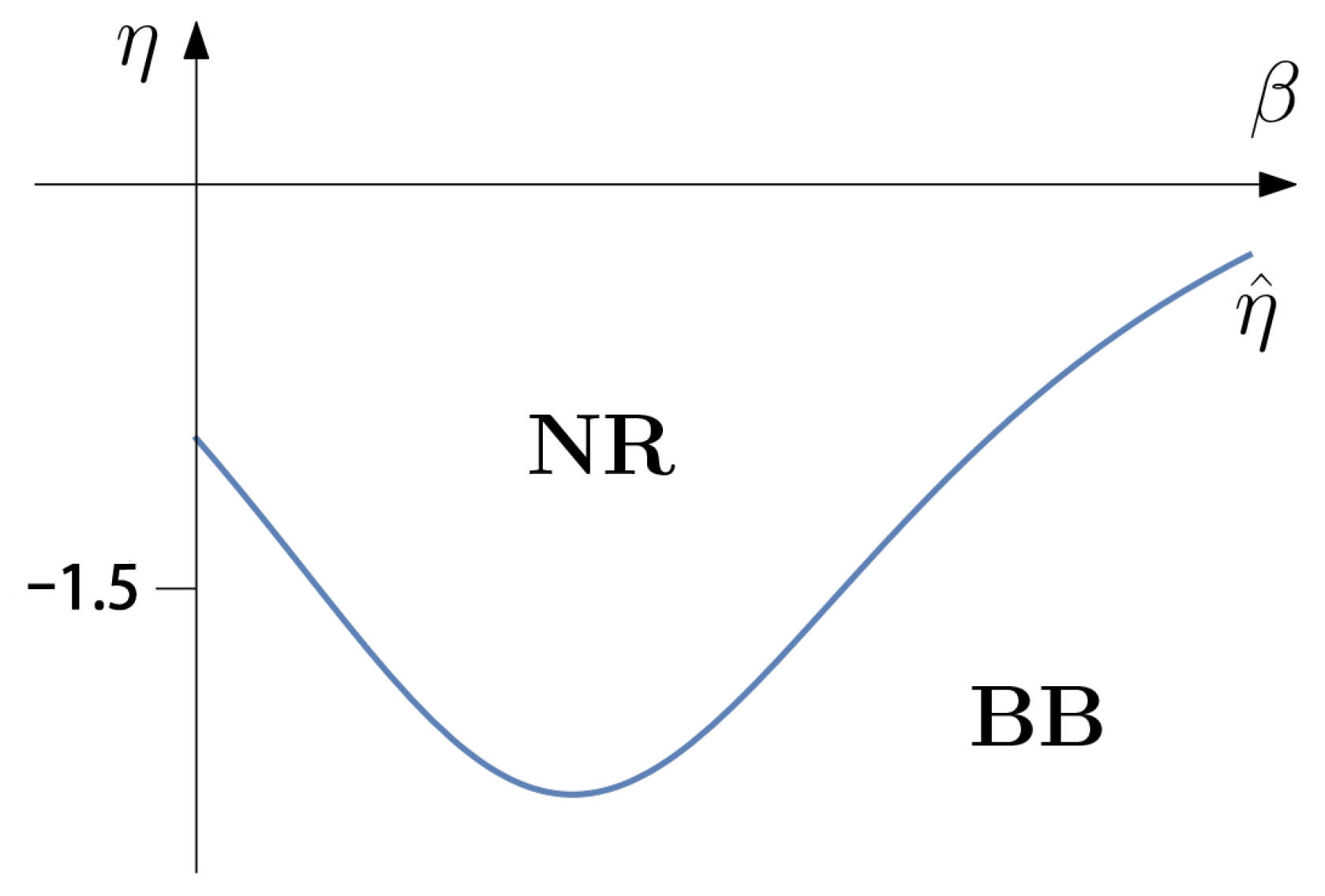
Figure 1. The equilibrium handling strategy, η and β 0 .
Jtaer 20 00282 g001
Figure 2. The impact of α 0 on p when η = 0.1 .
Jtaer 20 00282 g002
Figure 3. The impact of α 0 on p when η = 1 .
Jtaer 20 00282 g003
Figure 4. The impact of α 0 on T when η = 0.1 .
Jtaer 20 00282 g004
Figure 5. The impact of α 0 on w when η = 0.1 .
Jtaer 20 00282 g005
Figure 6. The impact of α 0 on D when η = 0.1 .
Jtaer 20 00282 g006
Figure 7. The impact of α 0 on R when η = 0.1 .
Jtaer 20 00282 g007
Figure 8. The impact of β 0 on p when η = 0.1 .
Jtaer 20 00282 g008
Figure 9. The impact of β 0 on p when η = 1 .
Jtaer 20 00282 g009
Figure 10. The impact of β 0 on π r .
Jtaer 20 00282 g010
Figure 11. The impact of β 0 on π m when η = 0.1 .
Jtaer 20 00282 g011
Figure 12. The impact of β 0 on π m when η = 1 .
Jtaer 20 00282 g012
Figure 13. The impact of η on π M S .
Jtaer 20 00282 g013
Figure 14. The impact of η on π R S .
Jtaer 20 00282 g014
Table 1. Notations.
Table 1. Notations.
Decision Variables
pUnit price
mProfit margin
TPromised delivery lead time (PDL)
wUnit wholesale price
DDemand function
RProduct returns function
π Profit function
Parameters
d 0 Market base
s 1 , s 2 Demand sensitivity to price and PDL, respectively
α 0 The maximum return rate
β 0 Return rate sensitivity to PDL
η Reselling ratio, which equals the margin of the reselling returned units scaled
by the magin of the regular selling units
cUnit cost
Table 2. The equilibrium solutions in the RS supply chain.
BB NR
m d 0 β 0 + s 2 ( 1 α 0 ) 3 s 1 β 0 c 3 β 0 ( 1 η ) d 0 c s 1 + s 2 α 0 η α 0 + 1 3 β 0 ( 1 η ) s 1
T d 0 c s 1 3 s 2 2 ( 1 α 0 ) 3 β 0 d 0 c s 1 3 s 2 2 ( 1 α 0 ( 1 η ) ) 3 β 0 ( 1 η )
w d 0 β 0 + s 2 ( 1 α 0 ) 6 s 1 β 0 + 5 c 6 β 0 ( 1 η ) d 0 + s 2 α 0 η α 0 + 1 6 β 0 ( 1 η ) s 1 + 5 c 6
π , m β 0 d 0 c s 1 + 1 α 0 s 2 3 108 β 0 2 s 1 s 2 β 0 ( 1 η ) d 0 c s 1 α 0 ( 1 η ) s 2 + s 2 2 36 β 0 2 ( 1 η ) 2 s 1
π , r β 0 d 0 c s 1 + 1 α 0 s 2 3 54 β 0 2 s 1 s 2 β 0 ( 1 η ) d 0 c s 1 α 0 ( 1 η ) s 2 + s 2 3 54 β 0 2 ( 1 η ) 2 s 1 s 2
Disclaimer/Publisher’s Note: The statements, opinions and data contained in all publications are solely those of the individual author(s) and contributor(s) and not of MDPI and/or the editor(s). MDPI and/or the editor(s) disclaim responsibility for any injury to people or property resulting from any ideas, methods, instructions or products referred to in the content.