
Analysis of Bullwhip Effect and Inventory Cost in an Omnichannel Supply Chain


Abstract
1. Introduction
- (1)
- How to optimize the BWE and inventory costs for omnichannel retailers across various supply chain contexts?
- (2)
- What are the formation mechanisms and mitigation measures of the BWE in omnichannel supply chains, considering their differences in the characteristics?
- (3)
- How do the pick-up lead time and return rate in the BOPS channel influence the BWE and inventory costs in omnichannel supply chains?
2. Literature Review
2.1. Bullwhip Effect
2.2. Omnichannel Retailing
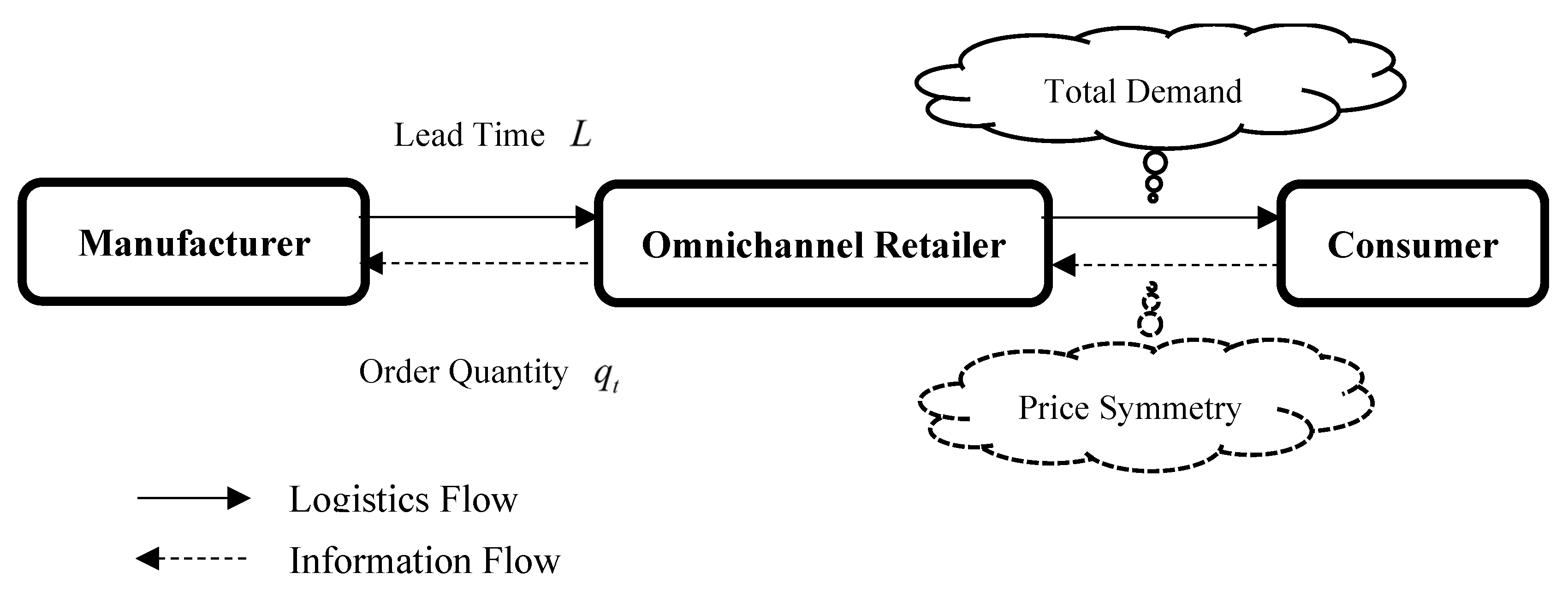
3. Demand Model
4. Ordering Decision
4.1. Inventory Strategy and Forecasting Technique
4.2. Ordering Decision of the Omnichannel Retailer
5. Bullwhip Effect and Expected Cost
5.1. Bullwhip Effect of the Omnichannel Retailer
5.2. Inventory Cost of the Omnichannel Retailer
5.3. Comparative Analysis
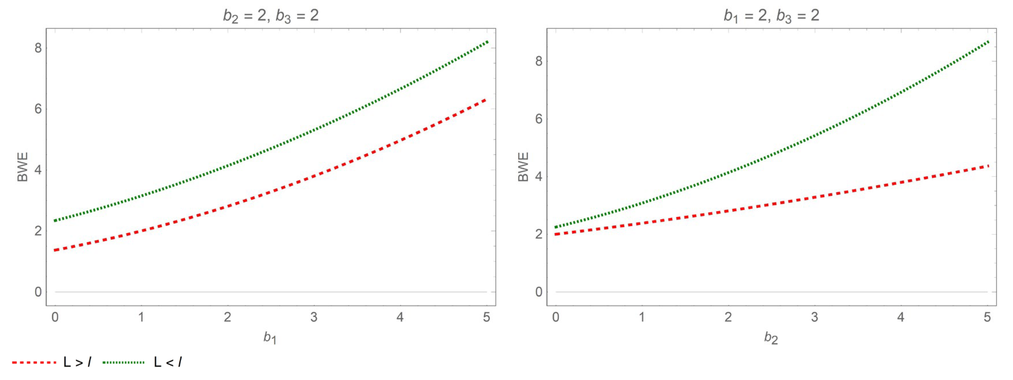
- (a)
- When , in the interval , . Therefore, increases with the price sensitivity coefficient .
- (b)
- When , in the interval , . Therefore, increases with the price sensitivity coefficient .
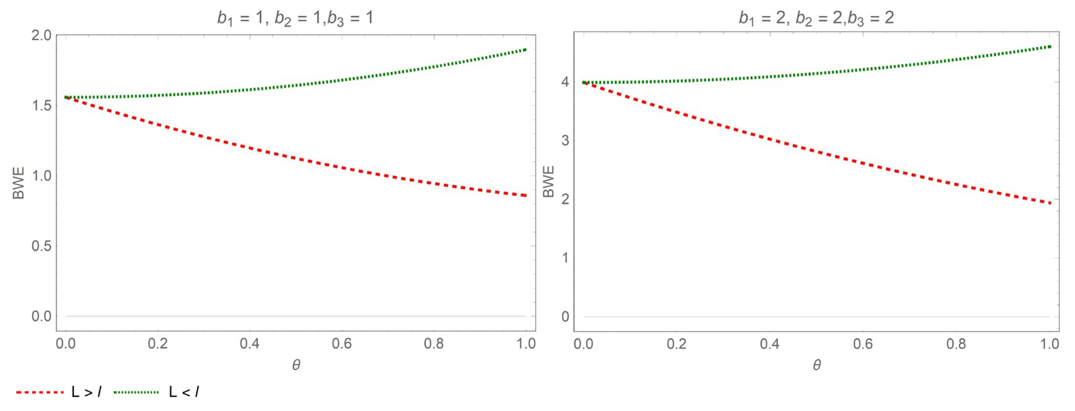
- (a)
- When , in the interval , . Therefore, decreases with the return rate .
- (b)
- When , in the interval , . Therefore, increases with the return rate .
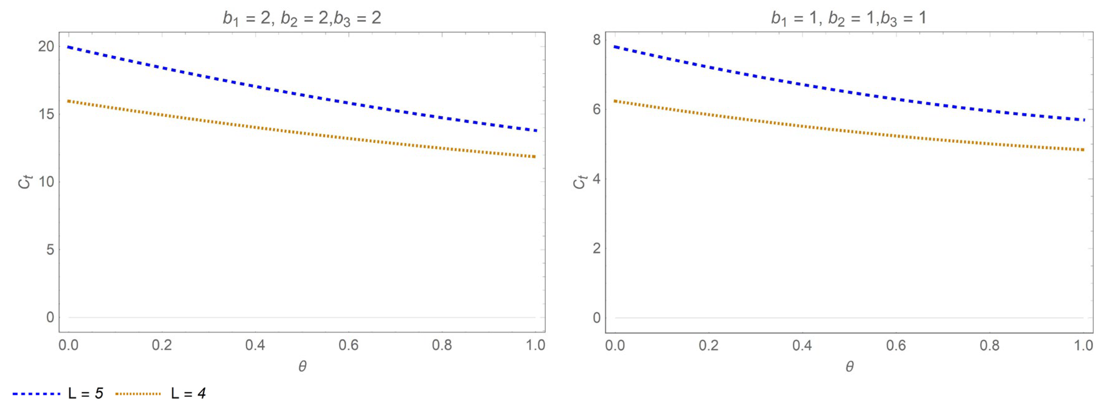
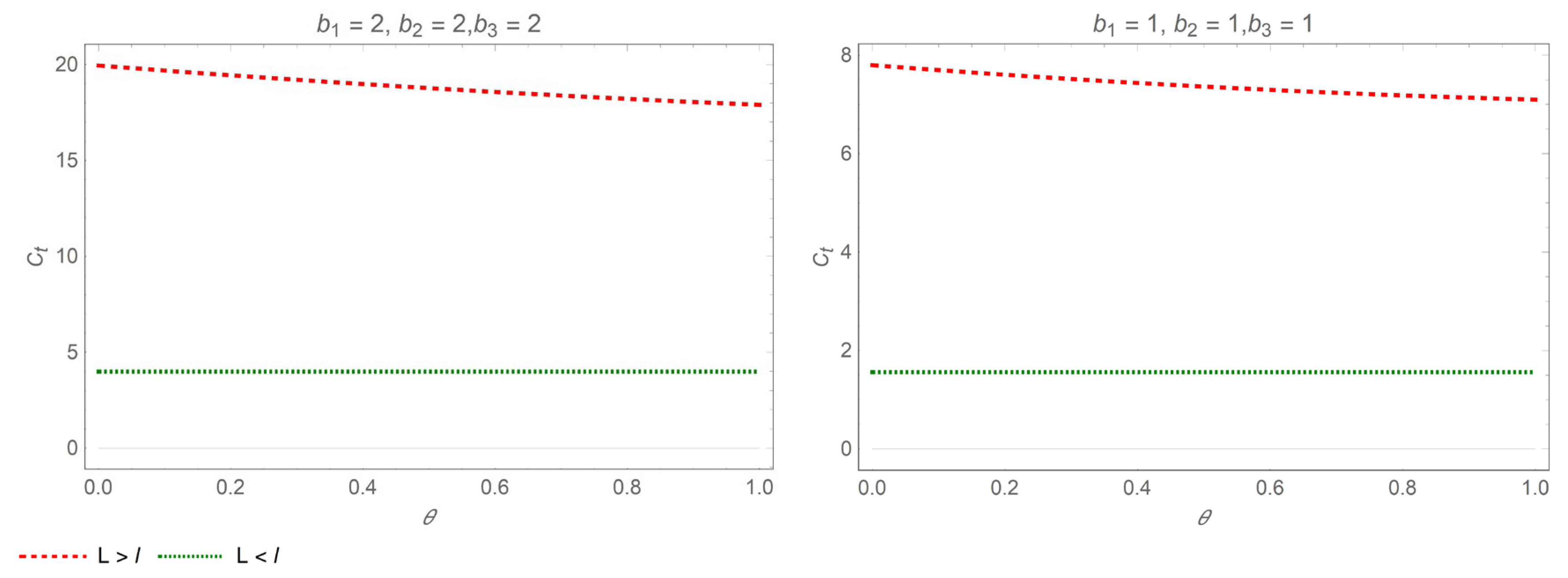
- (a)
- When , in the interval , . Therefore, the inventory cost diminishes with the return rate .
- (b)
- When , in the interval , the inventory cost is not correlated with the return rate .
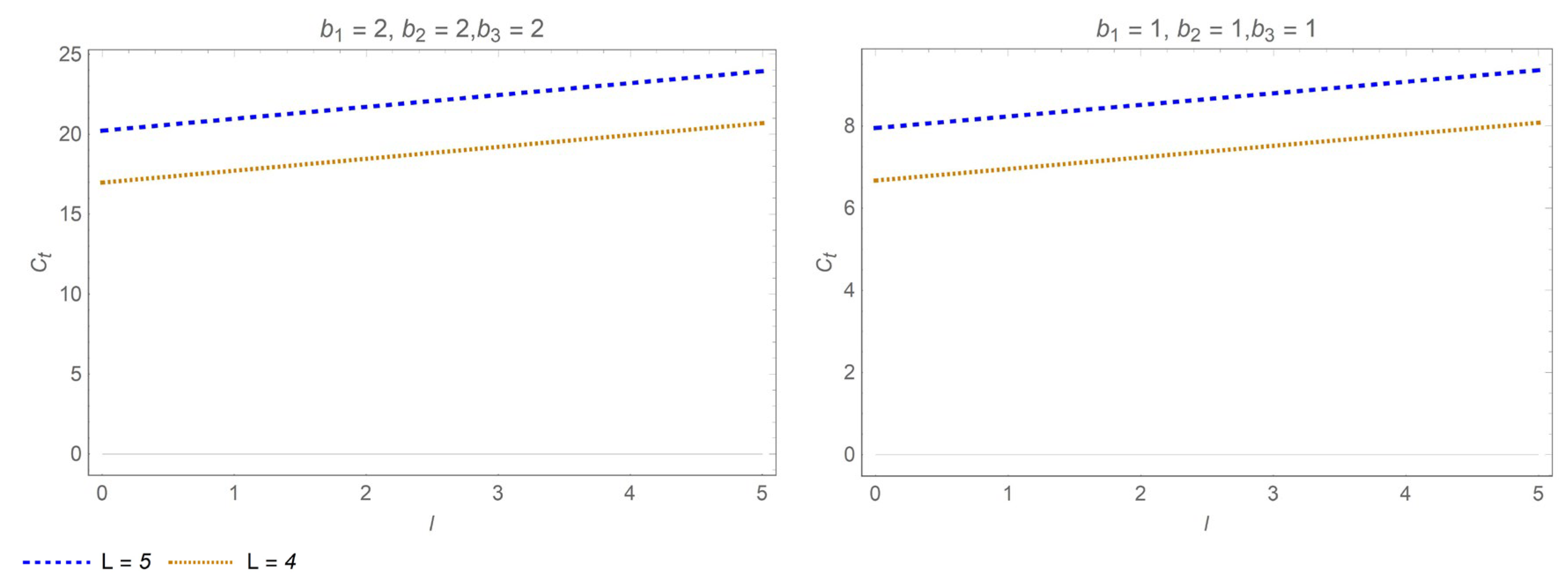
- (a)
- When , in the interval , . Therefore, the inventory cost is positively correlated with the pick-up lead time .
- (b)
- When , in the interval , the inventory cost is not correlated with the pick-up lead time .
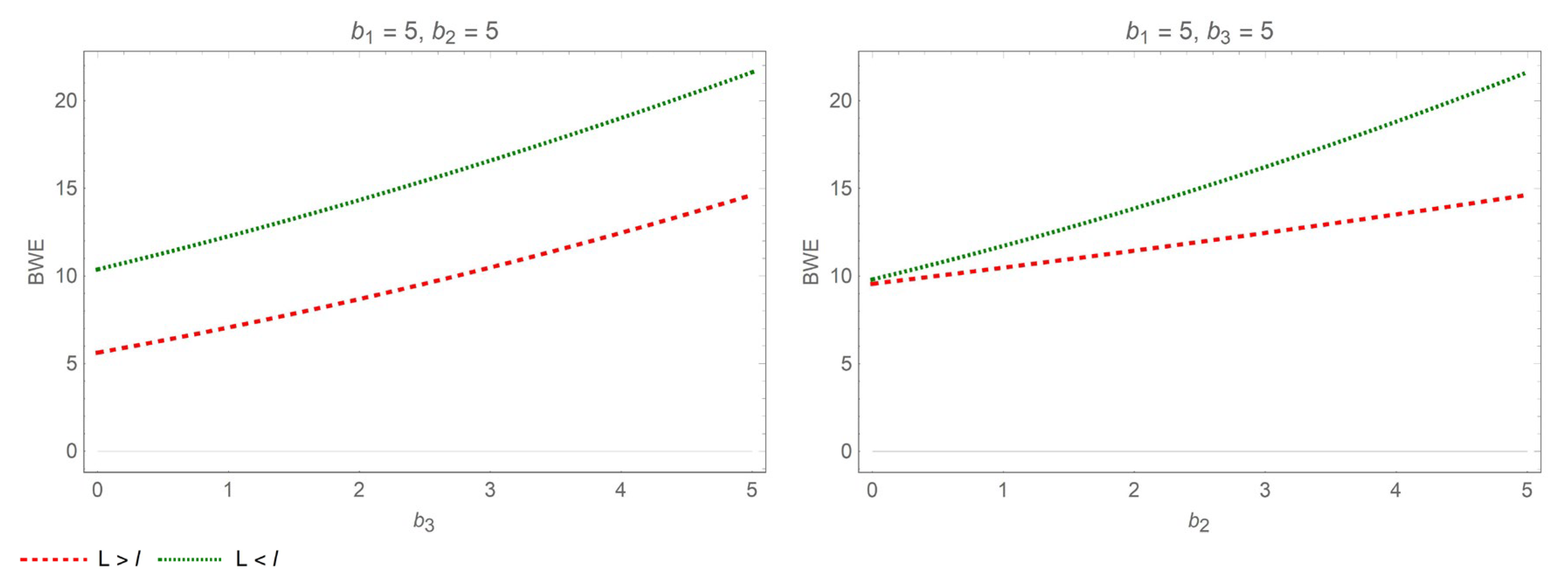
- (a)
- When , in the interval , . Therefore, expected cost increases with price sensitivity coefficient .
- (b)
- When , in the interval , . Therefore, expected cost increases with price sensitivity coefficient .
6. Conclusions and Limitations
6.1. Conclusions
6.2. Limitation
Author Contributions
Funding
Institutional Review Board Statement
Informed Consent Statement
Data Availability Statement
Conflicts of Interest
Abbreviations
| BWE | Bullwhip effect |
| BOPS | Buy online and pick up in store |
| MMSE | Minimum mean squared error |
| ARMA | Auto-regressive moving average |
| ES | Exponential smoothing |
| MA | Moving average |
| Normal i.i.d. | Independent and identically normally distributed |
Appendix A
Appendix B
Appendix C
Appendix D
Appendix E
References
- Wan, Y.C.; Yan, Z.P.; Wang, S.D. Pricing and return strategies in omni-channel apparel retail considering the impact of fashion level. Mathematics 2025, 13, 890. [Google Scholar] [CrossRef]
- Jin, M.; Li, G.; Cheng, T. Buy online and pick up in-store: Design of the service area. Eur. J. Oper. Res. 2018, 268, 613–623. [Google Scholar] [CrossRef]
- Silbermayr, L.; Waitz, M. Omni-channel inventory management of perishable products under transshipment and substitution. Int. J. Prod. Econ. 2024, 267, 109089. [Google Scholar] [CrossRef]
- Shih, D.H.; Huang, F.C.; Chieh, C.Y.; Shih, M.H.; Wu, T.W. From a Multichannel to an Optichannel Strategy in Retail. J. Theor. Appl. Electron. Commer. Res. 2025, 16, 2170–2191. [Google Scholar] [CrossRef]
- Basak, S.; Basu, P.; Avittathur, B.; Sikdar, S. A game theoretic analysis of multichannel retail in the context of “showrooming”. Decis. Support Syst. 2017, 103, 34–45. [Google Scholar] [CrossRef]
- Gao, D.; Wang, N.; Jiang, B.; Gao, J.; Yang, Z. Value of information sharing in online retail supply chain considering product loss. IEEE Trans. Eng. Manag. 2022, 69, 2155–2172. [Google Scholar] [CrossRef]
- Zhao, Y.; Li, Y.H.; Yao, Q.; Guan, X. Dual-channel retailing strategy vs. omni-channel buy-online-and-pick-up-in-store behaviors with reference freshness effect. Int. J. Prod. Econ. 2023, 263, 108967. [Google Scholar]
- Kim, S.; Connerton, T.P.; Park, C. Transforming the automotive retail: Drivers for customers’ omnichannel BOPS (Buy Online & Pick up in Store) behavior. J. Bus. Res. 2022, 139, 411–425. [Google Scholar]
- Goedhart, J.; Haijema, R.; Akkerman, R. Modelling the influence of returns for an omni-channel retailer. Eur. J. Oper. Res. 2023, 306, 1248–1263. [Google Scholar] [CrossRef]
- Goedhart, J.; Haijema, R.; Akkerman, R.; de Leeuw, S. Replenishment and fulfilment decisions for stores in an omni-channel retail network. Eur. J. Oper. Res. 2023, 311, 1009–1022. [Google Scholar] [CrossRef]
- Hense, J.; Hübner, A. Assortment optimization in omni-channel retailing. Eur. J. Oper. Res. 2022, 301, 124–140. [Google Scholar] [CrossRef]
- Gao, F.; Agrawal, V.; Cui, S. The effect of multichannel and omnichannel retailing on physical stores. Manag. Sci. 2022, 63, 2478–2492. [Google Scholar] [CrossRef]
- Cui, G.; Imura, N.; Nishinari, K. Should firms invest in demand forecasting? Benefits of improving forecasting accuracy on order smoothing, dual-sourcing and multi-stage supply chain problems. Int. J. Prod. Res. 2025, 59, 3323–3337. [Google Scholar] [CrossRef]
- Darmawan, A.; Wong, H.W.; Fransoo, J. Supply chain network design with the presence of the bullwhip effect. Int. J. Prod. Econ. 2025, 286, 109668. [Google Scholar] [CrossRef]
- Jalali, H.; Menezes, M.B. Product portfolio adjustments and the bullwhip effect: The impact of product introduction and retirement. Eur. J. Oper. Res. 2024, 318, 87–99. [Google Scholar] [CrossRef]
- Li, Q.Y.; Gaalman, G.; Disney, S.M. Dynamic analysis of the proportional order-up-to policy with damped trend forecasts. Int. J. Prod. Econ. 2025, 286, 109612. [Google Scholar] [CrossRef]
- Rozhkov, M.; Alyamovskaya, N.; Zakhodiakin, G. The beer game bullwhip effect mitigation: A deep reinforcement learning approach. Int. J. Prod. Res. 2025, 59, 3323–3337. [Google Scholar] [CrossRef]
- Yin, X.; Tang, W. The value of market information and the bullwhip effect. J. Oper. Res. Soc. 2024, 75, 2241–2252. [Google Scholar] [CrossRef]
- Zhan, Q.U.; Horst, R.A. Two-part tariffs, inventory stockpiling, and the bullwhip effect. Eur. J. Oper. Res. 2023, 308, 201–214. [Google Scholar]
- Lee, S.; Park, S.J.; Seshadri, S. Variations of the bullwhip effect across foreign subsidiaries. Manuf. Serv. Oper. Manag. 2023, 25, 1–8. [Google Scholar] [CrossRef]
- Lee, H.L.; Padmanabhan, V.; Whang, S. Information Distortion in a Supply Chain: The Bullwhip Effect. Manag. Sci. 1997, 43, 546–558. [Google Scholar] [CrossRef]
- Chen, F.; Simchi-Levi, D. Quantifying the Bullwhip Effect in a Simple Supply Chain: The Impact of Forecasting, Lead Times, and Information. Manag. Sci. 2000, 46, 436–443. [Google Scholar] [CrossRef]
- Lee, H.L.; So, K.C.; Tang, C.S. The Value of Information Sharing in a Two-Level Supply Chain. Manag. Sci. 2000, 46, 626–643. [Google Scholar] [CrossRef]
- Gao, D.; Wang, N.; He, Z.; Zhou, L. Analysis of bullwhip effect and inventory cost in the online closed-loop supply chain. Int. J. Prod. Res. 2023, 61, 6808–6828. [Google Scholar] [CrossRef]
- Patil, C.; Prabhu, V. Supply chain cash-flow bullwhip effect: An empirical investigation. Int. J. Prod. Econ. 2024, 267, 109065. [Google Scholar] [CrossRef]
- Pournader, M.; Narayanan, A.; Keblis, M.F.; Ivanov, D. Decision bias and bullwhip effect in multiechelon supply chains: Risk preference models. IEEE Trans. Eng. Manag. 2023, 71, 9229–9243. [Google Scholar] [CrossRef]
- Wang, X.; Disney, S.M. The bullwhip effect: Progress, trends and directions. Eur. J. Oper. Res. 2016, 250, 691–701. [Google Scholar] [CrossRef]
- Cannella, S.; Ponte, B.; Dominguez, R.; Framinan, J.M. Proportional order-up-to policies for closed-loop supply chains: The dynamic effects of inventory controllers. Int. J. Prod. Res. 2021, 59, 3323–3337. [Google Scholar] [CrossRef]
- Wang, N.; Lu, J.; Feng, G.; Ma, Y.; Liang, H. The bullwhip effect on inventory under different information sharing settings based on price-sensitive demand. Int. J. Prod. Res. 2016, 54, 4043–4064. [Google Scholar] [CrossRef]
- Hosoda, T.; Disney, S.M. A unified theory of the dynamics of closed-loop supply chains. Eur. J. Oper. Res. 2018, 269, 313–326. [Google Scholar] [CrossRef]
- Lingkon, M. Bullwhip effect on closed-loop supply chain considering lead time and return rate: A study from the perspective of Bangladesh. Decis. Sci. Lett. 2024, 13, 565–586. [Google Scholar] [CrossRef]
- Teunter, R.H.; Babai, M.Z.; Bokhorst, J.A.; Syntetos, A.A. Revisiting the value of information sharing in two-stage supply chains. Eur. J. Oper. Res. 2018, 270, 1044–1052. [Google Scholar] [CrossRef]
- Sun, S.Y.; Wang, N.M.; Xu, Y.F. Enhancing information transparency of online used car transactions through virtual reality in a competitive market. J. Ind. Manag. Optim. 2025, 21, 3310–3338. [Google Scholar] [CrossRef]
- Nagaraja, C.H.; McElroy, T. The multivariate bullwhip effect. Eur. J. Oper. Res. 2018, 267, 96–106. [Google Scholar] [CrossRef]
- Ponte, B.; Framinan, J.M.; Cannella, S.; Dominguez, R. Quantifying the Bullwhip Effect in closed-loop supply chains: The interplay of information transparencies, return rates, and lead times. Int. J. Prod. Econ. 2020, 230, 107798. [Google Scholar] [CrossRef]
- Yang, Y.; Lin, J.; Liu, G.; Zhou, L. The behavioural causes of bullwhip effect in supply chains: A systematic literature review. Int. J. Prod. Econ. 2021, 236, 108120. [Google Scholar] [CrossRef]
- Weisz, E.; Herold, D.M.; Kummer, S. Revisiting the bullwhip effect: How can AI smoothen the bullwhip phenomenon? Int. J. Logist. Manag. 2023, 34, 98–120. [Google Scholar] [CrossRef]
- Papanagnou, C.I. Measuring and eliminating the bullwhip in closed loop supply chains using control theory and Internet of Things. Ann. Oper. Res. 2022, 310, 153–170. [Google Scholar] [CrossRef]
- Al-Sukhni, M.; Migdalas, A. The impact of information sharing factors on the bullwhip effect mitigation: A systematic literature review. Oper. Res. 2025, 25, 1–42. [Google Scholar] [CrossRef]
- Niu, Y.; Wu, J.; Jiang, S.; Jiang, Z. The bullwhip effect in servitized manufacturers. Manag. Sci. 2024, 71, 1–20. [Google Scholar] [CrossRef]
- Du, K.; Jia, F.; Chen, L. The impact of customers’ MD&A sentiment on the bullwhip effect: A dyadic buyer-supplier perspective. Int. J. Prod. Econ. 2025, 284, 109614. [Google Scholar]
- Ma, J.; Lou, W.; Wang, Z. Pricing strategy and product substitution of bullwhip effect in dual parallel supply chain: Aggravation or mitigation? RAIRO-Oper. Res. 2022, 56, 2093–2114. [Google Scholar] [CrossRef]
- Tai, P.D.; Duc, T.T.H.; Buddhakulsomsiri, J. Measure of bullwhip effect in supply chain with price-sensitive and correlated demand. Comput. Ind. Eng. 2019, 127, 408–419. [Google Scholar] [CrossRef]
- Giri, B.C.; Glock, C.H. The bullwhip effect in a manufacturing/remanufacturing supply chain under a price-induced non-standard ARMA(1,1) demand process. Eur. J. Oper. Res. 2022, 301, 458–472. [Google Scholar] [CrossRef]
- Tai, P.D.; Buddhakulsomsiri, J.; Duc, T.T.H. Revisiting measurement of compound bullwhip with asymmetric reference price. Comput. Ind. Eng. 2022, 172, 108510. [Google Scholar] [CrossRef]
- Ma, Y.; Wang, N.; He, Z.; Lu, J.; Liang, H. Analysis of the bullwhip effect in two parallel supply chains with interacting price-sensitive demands. Eur. J. Oper. Res. 2015, 243, 815–825. [Google Scholar] [CrossRef]
- Rigby, D. The future of shopping. Harv. Bus. Rev. 2011, 89, 65–76. [Google Scholar]
- Brynjolfsson, E.; Hu, Y.; Rahman, M.S. Battle of the Retail Channels: How Product Selection and Geography Drive Cross-Channel Competition. Manag. Sci. 2009, 55, 1755–1765. [Google Scholar] [CrossRef]
- Bell, D.R.; Gallino, S.; Moreno, A. How to Win in an Omnichannel World. MIT Sloan Manag. Rev. 2014, 56, 45–53. [Google Scholar]
- Gao, F.; Su, X. Omnichannel Retail Operations with Buy-Online-and-Pick-up-in-Store. Manag. Sci. 2017, 63, 2478–2492. [Google Scholar] [CrossRef]
- Wang, K.; Li, Y.T.; Zhou, Y.L. Execution of Omni-Channel Retailing Based on a Practical Order Fulfillment Policy. J. Theor. Appl. Electron. Commer. Res. 2022, 17, 1185–1203. [Google Scholar] [CrossRef]
- Bayram, A.; Cesaret, B. Order fulfillment policies for ship-from-store implementation in omni-channel retailing. Eur. J. Oper. Res. 2021, 294, 987–1002. [Google Scholar] [CrossRef]
- Gallino, S.; Moreno, A. Integration of Online and Offline Channels in Retail: The Impact of Sharing Reliable Inventory Availability Information. Manag. Sci. 2014, 60, 1434–1451. [Google Scholar] [CrossRef]
- Kong, R.X.; Luo, L.; Chen, L.X.; Keblis, M.F. The effects of BOPS implementation under different pricing strategies in omnichannel retailing. Transp. Res. Part E: Logist. Transp. Rev. 2020, 141, 102014. [Google Scholar] [CrossRef]
- Zhang, J.; Xu, Q.; He, Y. Omnichannel retail operations with consumer returns and order cancellation. Transp. Res. Part E Logist. Transp. Rev. 2018, 118, 308–324. [Google Scholar] [CrossRef]
- Cocco, H.; Demoulin, N.T. Designing a seamless shopping journey through omnichannel retailer integration. J. Bus. Res. 2022, 150, 461–475. [Google Scholar] [CrossRef]
- Qiu, R.; Yuan, M.; Sun, M.; Fan, Z.P.; Xu, H. Optimizing omnichannel retailer inventory replenishment using vehicle capacity-sharing with demand uncertainties and service level requirements. Eur. J. Oper. Res. 2025, 320, 417–432. [Google Scholar] [CrossRef]

| Forecasting Technique | Model Formulation | Advantages of the Technique |
|---|---|---|
| MMSE | Lowest prediction error and highest accuracy [18,21,23,24,27,29,30,34,35] | |
| MA | * | Simple calculation and clear trends [20,22,27,32] |
| ES | * | Recent data focus and quick adaptation [14,26,27,28] |
| Studies on Bullwhip Effect | Demand Model | Price Model | Supply Chain Contexts |
|---|---|---|---|
| Tai et al. [43,45] | Price-sensitive AR(1) demand | Normal i.i.d | Simplified supply chain with a single retail channel |
| Ma et al. [42] | Price-sensitive demand | VAR(1) | Complex supply chain with multiple retail channels |
| Giri et al. [44] | Price-sensitive demand | ARMA(1,1) | Complex supply chain with a single retail channel |
| Gao et al. [24] | Normal i.i.d | \ | Complex supply chain with a single retail channel |
| Ponte et al. [35], Papanagnou [38] | Normal i.i.d | \ | Complex supply chain with a single retail channel |
| Wang et al. [46] | Price-sensitive demand | AR(1) | Complex supply chain with multiple retail channels |
| This study | Price-sensitive demand | Normal i.i.d | Simplified supply chain with omnichannel |
| Studies on Omnichannel | Price Information Symmetry | Pricing Strategy in Omnichannel |
|---|---|---|
| Jin et al. [2], Silbermayr and Waitz [3], Goedhart et al. [9,10], Gao et al. [12], Gao and Su [50], Cocco and Demoulin [56] | Symmetry | Uniform pricing |
| Basak et al. [5], Kim et al. [8] | Symmetry | Differentiated pricing |
| Zhao et al. [7] | Asymmetry | Differentiated pricing |
| This study | Symmetry | Uniform pricing |
Disclaimer/Publisher’s Note: The statements, opinions and data contained in all publications are solely those of the individual author(s) and contributor(s) and not of MDPI and/or the editor(s). MDPI and/or the editor(s) disclaim responsibility for any injury to people or property resulting from any ideas, methods, instructions or products referred to in the content. |
© 2025 by the authors. Licensee MDPI, Basel, Switzerland. This article is an open access article distributed under the terms and conditions of the Creative Commons Attribution (CC BY) license (https://creativecommons.org/licenses/by/4.0/).
Share and Cite
Gao, D.; Liu, C.; Sun, X. Analysis of Bullwhip Effect and Inventory Cost in an Omnichannel Supply Chain. J. Theor. Appl. Electron. Commer. Res. 2025, 20, 182. https://doi.org/10.3390/jtaer20030182
Gao D, Liu C, Sun X. Analysis of Bullwhip Effect and Inventory Cost in an Omnichannel Supply Chain. Journal of Theoretical and Applied Electronic Commerce Research. 2025; 20(3):182. https://doi.org/10.3390/jtaer20030182
Chicago/Turabian StyleGao, Dandan, Chenhui Liu, and Xinye Sun. 2025. "Analysis of Bullwhip Effect and Inventory Cost in an Omnichannel Supply Chain" Journal of Theoretical and Applied Electronic Commerce Research 20, no. 3: 182. https://doi.org/10.3390/jtaer20030182
APA StyleGao, D., Liu, C., & Sun, X. (2025). Analysis of Bullwhip Effect and Inventory Cost in an Omnichannel Supply Chain. Journal of Theoretical and Applied Electronic Commerce Research, 20(3), 182. https://doi.org/10.3390/jtaer20030182