Forecasting Sales in Live-Streaming Cross-Border E-Commerce in the UK Using the Temporal Fusion Transformer Model

Abstract

As globalization deepens and the digital economy rapidly develops, cross-border e-commerce, especially live-streaming e-commerce, has emerged as a significant driver of international trade growth. However, the highly unpredictable sales demand in this sector and external factors such as the COVID-19 pandemic and Brexit have posed significant challenges in accurately forecasting sales within the UK live-streaming e-commerce market. To address these challenges, we propose a novel sales forecasting framework utilizing the Temporal Fusion Transformer (TFT) model. Our multimodal approach integrates diverse time series data, including historical sales, key opinion leader (KOL) influence, and seasonal patterns. The Temporal Fusion Transformer (TFT) model demonstrated consistently lower Mean Absolute Error (MAE), Root Mean Squared Error (RMSE), and Mean Squared Error (MSE) across all forecasting horizons compared to other machine learning approaches, including Long Short-Term Memory (LSTM), Convolutional Neural Networks (CNN), and Gated Recurrent Unit(GPU)-accelerated architectures. Furthermore, it exhibited significantly superior performance over traditional time-series methods such as the Autoregressive Integrated Moving Average (ARIMA) model. This research proposes a phased framework for short-term, medium-term, and long-term forecasting, providing a fresh perspective for product forecasting studies and offering significant theoretical support for cross-border e-commerce enterprises in product life cycle management.

1. Introduction

In the context of rapid global value chain restructuring, cross-border e-commerce is emerging as a significant driver of growth in international trade, fundamentally changing traditional trade patterns [1,2,3]. According to the Office for National Statistics (ONS) in the United Kingdom (UK), the proportion of UK exports destined for the European Union (EU) declined to 42% in 2023, marking a structural reduction from the 2010 pre-Brexit baseline of 47.3% (Source: Data from ONS series FSL4, FSIK, L854 and IKBB). According to the Office for National Statistics Pink Book 2024, the shift in market focus has led UK cross-border e-commerce to adopt diversification strategies that increasingly direct resources towards North America, China, and Australia.

The significant changes in the institutional environment have created a dual effect. On the one hand, the coronavirus disease 2019 (COVID-19) pandemic [4,5], supply chain reconfiguration [6,7], escalation of tariff barriers, and fragmentation of regulatory rules have exacerbated operational complexities, exemplified by the policy differentiation of digital platforms such as TikTok Shop—UK exporters to the EU face commission rates of 5–8%, compared to 2–5% for EU-based sellers (Source: https://www.shoplazza.com/blog/eu-crossborder-sellers-on-tiktok-shop (accessed on 28 April 2025)). On the other hand, the sustained depreciation of the British pound post-Brexit has enhanced the attractiveness of UK cross-border e-commerce to global consumers [8]. Despite the short-term shocks induced by Brexit, it has also presented opportunities for UK cross-border e-commerce to optimize its international market deployment [9,10,11].

In recent years, the rapid development of short video platforms and live-streaming technology has given rise to the emerging model of cross-border live-streaming e-commerce [12]. Live streaming e-commerce has significantly improved consumer conversion rates through instant interaction and immersive shopping experience, becoming an essential sales method for cross-border e-commerce [13,14,15]. However, cross-border live-streaming sales face many uncertainties, such as the cyclical nature of live-streaming activities, seasonality, and fluctuations in macroeconomic factors [16,17]. As a unique form of cross-border e-commerce, live streaming not only faces the challenges of ordinary cross-border e-commerce but also the impact of multimodal factors such as product display, inventory, logistics chain, the influence of anchors, and real-time interaction on sales cannot be ignored. Therefore, achieving accurate sales forecasts in this volatile market environment is essential for cross-border e-commerce companies.

Although the Autoregressive Integrated Moving Average model (ARIMA) is a widely used statistical method for time series forecasting, it is weak in processing complex nonlinear data features [18,19]. The ARIMA model has difficulty dealing with seasonality, emergencies, and multivariable interaction effects in cross-border e-commerce live broadcast data [20,21]. With the development of machine learning technology, deep learning models have shown substantial advantages in sales forecasting scenarios. However, their “black box” characteristics make the model less interpretable and challenging to explain sufficiently to corporate decision-makers [22,23]. Consequently, improving sales forecasts’ accuracy and enhancing predictive models’ interpretability have emerged as critical challenges that cross-border e-commerce companies must address.

To address the above challenges of forecasting cross-border e-commerce live-streaming sales in the United Kingdom, this study employs the Temporal Fusion Transformer (TFT) model, a cutting-edge approach that integrates deep learning with time series analysis [24]. The TFT model has the ability of traditional forecasting models to process multivariate time series and efficiently process complex time series data through its innovative structure, especially in self-attention mechanism, feature selection, and seasonal modelling. In addition, TFT also significantly improves the interpretability of the model through feature importance analysis.

This study aims to explore and address two central research questions:

RQ1: Does the Temporal Fusion Transformer (TFT) outperform the traditional ARIMA model in forecasting sales for cross-border e-commerce live streaming in the UK?

RQ2: What factors significantly influence sales performance in cross-border e-commerce live streaming within the UK market? Beyond historical sales data, can integrating factors such as Key Opinion Leader (KOL) influence, seasonality, and holiday effects improve the accuracy of sales forecasting models?

The primary contributions of this study are fourfold:

• Enhanced Temporal Fusion Transformer (TFT): The introduction of novel prediction position encodings optimizes the capture of long-term dependencies and local features in the data.
• Multi-feature data integration: This study presents a forecasting framework that integrates various data types—historical sales, KOL influence, user behavior, and seasonal features—resulting in improved prediction accuracy.
• Improved Model Interpretability: The model incorporates concepts of long-term, medium-term, and short-term predictions, significantly enhancing the model’s interpretative capabilities and facilitating more optimized decision-making throughout the entire life cycle management of cross-border e-commerce.
• Industry Relevance: The proposed model offers cross-border e-commerce businesses a more effective tool to navigate the volatile market environment and enhance operational efficiency.

The structure of the paper is as follows: Section 2 reviews relevant literature; Section 3 details the Temporal Fusion Transformer model and the feature selection process; Section 4 outlines the experimental design and results analysis; and Section 5 summarizes the conclusions and discusses potential avenues for future research.

2. Theoretical Analysis of E-Commerce Demand Fluctuations

2.1. Demand Forecasting

Demand forecasting is crucial in cross-border e-commerce, especially in the fast-paced realm of live-streaming commerce [25,26,27]. Accurate forecasting allows merchants to optimize inventory, improve operations, and boost customer satisfaction [28,29].

Based on existing academic research, scholars usually divide e-commerce sales forecasting methods into qualitative and quantitative categories. Qualitative methods depend on the subjective judgment of experts and insights into market trends [30,31]. In contrast, quantitative methods include traditional multivariate regression models, time series forecasting techniques like ARIMA, and modern machine learning algorithms such as random forests and neural networks, which have gained popularity recently. These quantitative methods analyze historical data to identify sales patterns and predict future trends [32,33,34]. Factors such as data availability, the complexity of sales patterns, and the level of accuracy required in the forecasts typically influence the selection of a forecasting model.

Traditional time series forecasting models, such as ARIMA and exponential smoothing, have been widely used in sales forecasting [35,36]. However, these models often struggle to capture the inherent non-linearity and high-dimensional features in cross-border e-commerce data. In recent years, advancements in machine learning have made it possible to address the challenges of analyzing complex, unstructured, and multimodal data in this field. For instance, Elalem et al. (2023), Xie et al. (2024) and Chen et al. (2024). employ machine learning techniques such as Long Short-Term Memory (LSTM), Gated Recurrent Unit (GRU) and Convolutional Neural Network (CNN) to forecast sales [37,38,39]. The study concluded that deep learning models have significant advantages when handling complex sales data.

However, one drawback of existing machine-learning research is the lack of interpretability associated with black-box models. Therefore, this study proposes an enhanced Temporal Fusion Transformer (TFT) model and constructs a forecasting framework using features such as historical sales data, KOL influence, and seasonality to enhance sales forecasts’ accuracy and interpretability [24].

2.2. Factors Influencing E-Commerce Live-Streaming Sales

Given the findings of previous studies, historical data, KOL network externalities, seasonality, and weekend/holiday effects are significant determinants of product sales. Therefore, we put these factors into our forecasting model.

2.2.1. Historical Data

The cross-border e-commerce industry rapidly transforms the global business landscape as globalization advances. Although cross-border live-streaming e-commerce faces similar challenges to traditional cross-border e-commerce, it also faces the complexity of multimodal information [40]. In this complex cross-border e-commerce environment, accurate sales forecasting is crucial for companies to optimize supply chain management and sales-related decisions [41,42].

Previous research on cross-border e-commerce sales forecasting has consistently underpinned its models with historical sales data. For instance, Liu (2020) developed a time series prediction model that integrated external observable data and hidden Markov models to capture latent features in historical sales data better, improving prediction reliability [43]. Chen (2023) examined the predictive power of historical data in the baby food sector by extracting key features, such as current prices and seven-day moving sales averages [44]. The study used a Gaussian process model and demonstrated the significant contribution of historical data to forecasting accuracy.

2.2.2. Influence of Key Opinion Leaders (KOLs)

The personal charisma, product demonstrations, and real-time engagement of Key Opinion Leaders (KOLs) have enhanced product stickiness among followers on live-streaming e-commerce platforms. Scholars call this effect the KOL network effect. As KOLs’ influence expands, it can promote the growth of fan groups, attract more potential consumers’ attention, and promote purchasing behavior through the scale effect [45,46,47].

Empirical studies have consistently demonstrated the significant spillover effect that Key Opinion Leaders (KOLs) have on consumer purchasing behavior. One valuable framework for understanding this influence is the Dual-Systems Theory (DST). DST posits that consumer decisions are shaped by two systems: the affective system, which drives quick, intuitive responses, and the cognitive system, which governs slower, more deliberative decision-making [48]. In this context, the personalities and behaviors of KOLs can evoke both emotional and rational responses in consumers, thereby significantly impacting their purchasing decisions.

Lin (2024) further explored the dual role of KOLs in live-stream sales, uncovering complex game-theoretic relationships between brands and KOLs [49]. KOLs with positive public images can significantly amplify a brand’s reach, while those entangled in damaging controversies can diminish brand reputation. For example, Liping Xiong (2021) conducted an in-depth study on how KOL characteristics, consumer attributes, and social media platforms influence the brand image of skincare products [50].

2.2.3. Seasonal Features

Numerous studies have highlighted the importance of considering seasonal fluctuations when predicting e-commerce product sales, as neglecting these factors can lead to significant errors [51,52]. As a result, many researchers focus on the seasonal characteristics of product sales in their analyses. For instance, Fathalla et al. (2020) employed Long Short-Term Memory (LSTM) and Seasonal Autoregressive Integrated Moving Average (SARIMA) methods to demonstrate that second-hand goods on e-commerce platforms exhibit seasonal sales peaks, thus addressing the limitations in feature representation seen in traditional ARIMA models [53]. Kharfan et al. (2021) further used machine learning technology to predict the demand for seasonal products and verified that seasonal characteristics significantly impact the accuracy of sales forecasts [54].

Forecasting cross-border e-commerce product demand is crucial for businesses to optimize inventory, pricing, and marketing strategies. Existing literature has explored various approaches to this challenge. Traditional time series models, such as Seasonal Autoregressive Integrated Moving Average (SARIMA), have been widely employed to capture trends and seasonality effectively. For example, Zhao (2024) demonstrated the robustness of SARIMA in accurately forecasting demand with pronounced seasonal patterns [55]. However, recent research has increasingly embraced machine learning techniques for their potential to capture complex non-linear relationships and adapt to dynamic market conditions. Tran and Huh (2023) investigated the Apriori algorithm and proposed the S-Apriori algorithm specifically tailored to model seasonal shopping behavior. This innovative approach has been successfully implemented to develop a robust consumer behavior prediction framework [56].

2.2.4. Weekend and Holiday Effects

The literature has extensively documented the impact of weekends and holidays on e-commerce sales. Previous studies in traditional e-commerce contexts have highlighted that holidays [57,58,59] and weekends [60,61,62] significantly influence consumer purchasing behavior due to variations in leisure time, social rituals, and spending motivations. However, with the rise of cross-border e-commerce live streaming, which features real-time interaction, personalized recommendations, social attributes, and entertainment, the existence of weekend and holiday effects warrants further investigation.

Consumer behavior research provides theoretical underpinnings for understanding these phenomena [62]. For instance, mental accounting theory suggests that consumers classify consumption behaviors into distinct mental accounts, leading them to perceive consumption during holidays or weekends as leisure and enjoyment. Holidays or weekends lower their consumption thresholds, making them more susceptible to promotional stimuli [63,64]. Additionally, the endowment effect, which describes consumers’ tendency to overvalue possessions, may diminish during these periods, fostering impulsive purchasing tendencies.

3. Methodology

3.1. Data

3.1.1. Data Description

The live shopping model of TikTok in the UK has a good market prospect, offering a valuable dataset to inform and enhance our sales forecasting model. As shown in Figure 1, TikTok’s user base is predominantly young with considerable purchasing power. This study uses the TikTok platform to forecast live sales of cross-border beauty and skincare e-commerce in the United Kingdom.

In this study, we employed Python and Youhou scripts to crawl detailed data of each live broadcast using the product ID of the UK cross-border e-commerce TikTok live broadcast sales, and we strictly abide by the platform’s privacy protection and data use regulations. The data collection process adhered solely to the platform’s privacy protection and data usage policies. Each data record includes the following fields:

• Basic product information: This section includes product name, category, and description.
• Live-streaming content: This section provides information on the live-streaming session, including the start time, end time, title, duration, price, and total number of viewers.

According to industry data released by Statista (2023), merchandise sales on the UK TikTok Shop platform in 2023 exhibited significant category differentiation, with beauty and personal care products accounting for 32% of the total market share and emerging as the leading product category (Source: based on Statistics 2024, https://www.statista.com/statistics/1536169/united-kingdom-goods-tiktok-shop-share/ (accessed on 6 January 2025)). Given the prominent market dominance demonstrated by this sector within the social commerce domain and its industry representativeness, this study selects beauty products as its primary research subject. The investigation aims to conduct an in-depth analysis of consumer behaviour patterns and evaluate the effectiveness of marketing strategies through this representative sample within social commerce platforms.

To ensure model accuracy, sales records of live broadcasts related to cross-border beauty and skincare e-commerce in the UK were collected over six months, from 1 January 2024 to 1 July 2024. This resulted in a dataset of 30,906 records, covering the entire cycle and full coverage data characteristics of the live broadcast platform.

Table 1. Data overview.

Field	Example
Country	British
Id	1729399984946253384
Category	Beauty and skincare
Price	USD 19.11
KOL name	@adaslifestyleb
Number of fans	12,000
Sale	36
Live streaming start time	1 June 2024 14:05:11
Live streaming end time	1 June 2024 17:55:53
Live streaming title	Time to do my nails
Live streaming duration	3 h 50 m
Number of viewers	17,906
Product Description	L’Oreal Skincare & Comfort Revitalift Filler
	Hyaluronic Acid & Caffeine Revitalift Eye Serum,
	Filler Plumping Water Cream, Anti-Wrinkle Dropper
	Serum Paradise Glotion Glow, Select your Type

provides an overview of the specific fields in a single data record with examples.

Figure 2 illustrates that the sales volume of live broadcasts for UK beauty and skincare products exhibits significant fluctuations, indicating non-stationary time series characteristics. Given that traditional ARIMA models assume stationarity, their performance is limited when handling such highly volatile datasets. Consequently, this study sets the ARIMA model as a baseline to evaluate the performance gains of the Temporal Fusion Transformer (TFT) method for time series forecasting.

3.1.2. Data Cleaning

To ensure data quality, we cleaned the sales data through the following steps: First, considering the independence of each live stream, imputation methods that fill in missing values were deemed likely to introduce substantial errors. Therefore, we removed records with missing data rather than imputing them. Second, aiming to identify general patterns in product sales and enhance data quality, we employed the interquartile range (IQR) method to clean the outliers in the dataset. Calculating the IQR and setting a reasonable multiplier eliminated extreme data points that could distort the analysis results.

3.2. Key Factors Influencing Prediction

This study investigates the impact of various feature variables on sales in cross-border live-streaming e-commerce on TikTok in the UK.

3.2.1. Live-Streaming Sales Features

Sales characteristics are vital in helping us understand product performance trends and forecast future demand.

• Original Sales (Sale): The historical sales data, denoted as Sale, serve as the primary indicator of fundamental sales trends over time.
• Log Sales (Log_sale): The natural logarithm of sales data (Log_sale) is employed to smooth fluctuations and reduce the influence of extreme values. To prevent computational issues with zero-valued sales, a small constant ($ϵ>0$) is added.
• Average Sales by Product ID (Average_Sale_by_ID): The average sales performance for each product ID is calculated as shown in Equation (1):

  $$\mathit{Avg\_Sale\_by\_ID}={\displaystyle \frac{1}{N_i}}\sum _{j=1}^{N_i}{\mathit{Sale}}_{i,j}$$

  (1)

  where $N_i$ represents the total number of records for product ID i, and ${\mathit{Sale}}_{i,j}$ denotes the sales value of the j-th record.

3.2.2. Key Opinion Leader (KOL) Features

These variables quantify the influence of live-streaming sessions and their hosts (KOLs):

• Live Streaming Price (Price): Prices are standardized using the exchange rate r, converting the original price p into USD, as shown in Equation (2):

  $$\mathit{Price}=p·r$$

  (2)
• Live Streaming Duration (Duration) [65]: Measured in minutes, where h and m denote hours and additional minutes, respectively, as shown in Equation (3):

  $$\mathit{Duration}=h·60+m$$

  (3)
• Number of Viewers (Views): Reflects the real-time audience size during a live stream, serving as a proxy for the KOL’s influence on sales.

3.2.3. Time Features

Temporal variables capture sequential and cyclic patterns in the data:

• Time Index (Time_idx): Represents the chronological sequence of records, ordered by time and product category.
• Relative Time Index (Relative_Time_idx): Denotes the position of the current time point relative to the sequence.
• Cyclic Features (Weekday_sin, Weekday_cos, Week_sin, Week_cos) [66]: To model periodic influences, sine and cosine transformations are applied as shown in Equations (4) and (5).

  $$\mathit{Weekday\_sin}=sin\left(2\pi ·{\displaystyle \frac{\mathit{Weekday}}{7}}\right),\mathit{Weekday\_cos}=cos\left(2\pi ·{\displaystyle \frac{\mathit{Weekday}}{7}}\right)$$

  (4)

  $$\mathit{Week\_sin}=sin\left(2\pi ·{\displaystyle \frac{\mathit{Week}}{52}}\right),\mathit{Week\_cos}=cos\left(2\pi ·{\displaystyle \frac{\mathit{Week}}{52}}\right)$$

  (5)
• Seasonality (Seasonality): Seasonal trends, particularly prominent for products such as sunscreen, are captured using the month of the transaction as shown in Equation (6):

  $$\mathit{Seasonality}=\mathrm{month}\left(\mathit{Time}\right)$$

  (6)

3.2.4. Weekend and Holiday Effects

The impact of weekends and holidays on consumer behavior is modeled using binary variables as described in Equations (7) and (8).

• Weekend Effect (Weekend): Indicates whether a record corresponds to a weekend:

  $$\mathit{Weekend}=\left\{\begin{array}{cc}1,\hfill & \mathit{if}\mathit{Saturday}\mathit{or}\mathit{Sunday},\hfill \\ 0,\hfill & \mathit{otherwise}.\hfill \end{array}\right.$$

  (7)
• Holiday Effect (Holiday): Captures the effects of national and cultural holidays:

  $$\mathit{Holidays}=\left\{\begin{array}{cc}1,\hfill & \mathit{if}\mathit{a}\mathit{local}\mathit{holiday},\hfill \\ 0,\hfill & \mathit{otherwise}.\hfill \end{array}\right.$$

  (8)

3.3. Model Design

This study aims to predict the sales of TikTok cross-border e-commerce live streaming in the UK. To provide a more comprehensive evaluation of the enhanced Temporal Fusion Transformer (TFT) model’s predictive performance, this research also employs the traditional e-commerce sales forecasting method, the ARIMA model, as a comparative control.

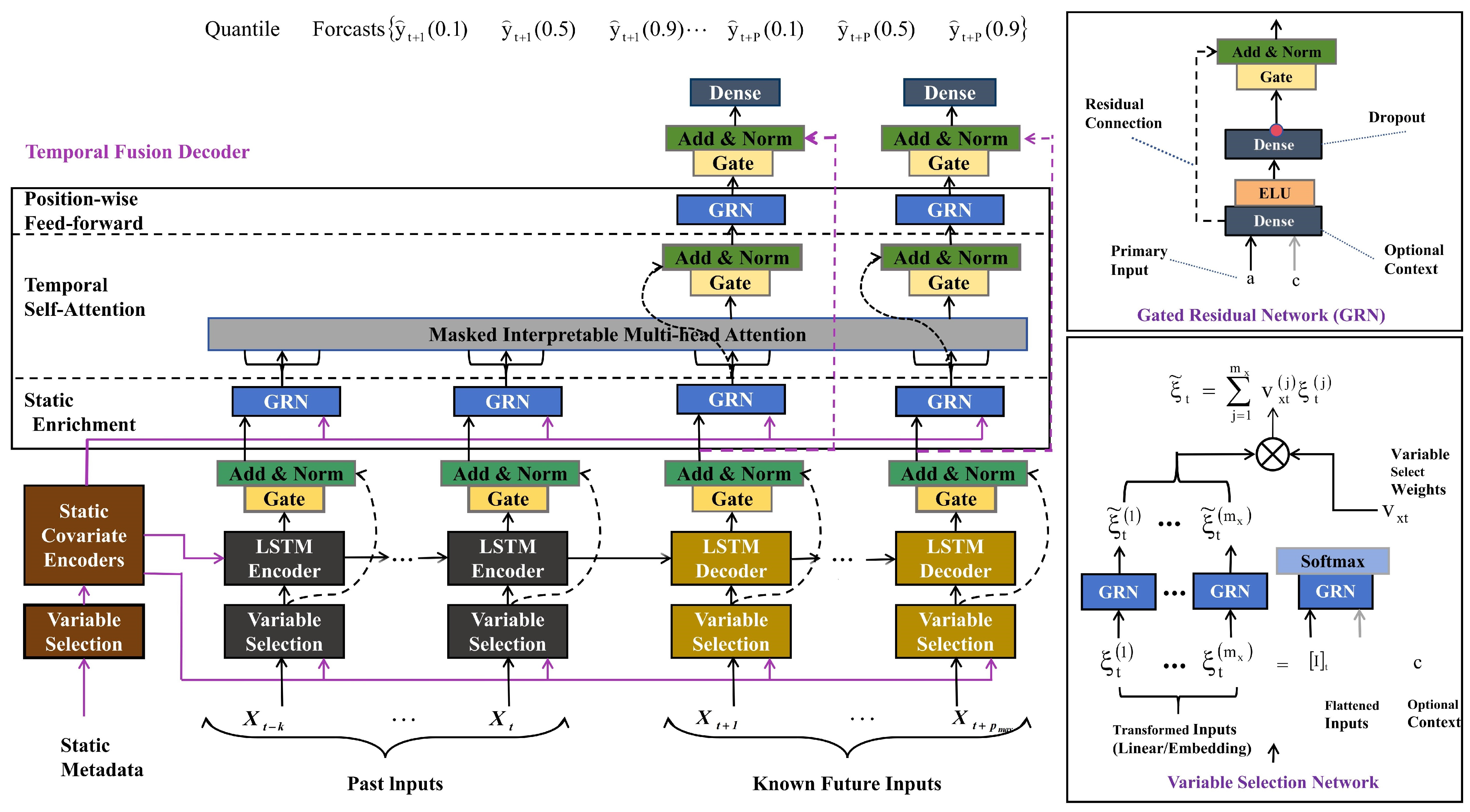
3.3.1. Temporal Fusion Transformer (TFT) Model

Unlike traditional “black box” models, such as neural networks or ensemble methods, the TFT model enhances interpretability by quantifying the contribution of each input feature to the prediction outcome through a gating mechanism and a variable selection network. Figure 3 illustrates the detailed structure of the model. Furthermore, Equation (9) mathematically defines the prediction function.

We consider a time series dataset composed of I distinct entities, where each entity i is associated with static covariates ${\mathbf{s}}_i\in {\mathbb{R}}^{m_s}$, dynamic inputs ${\chi }_{i,t}={\left[{\mathbf{O}}_{i,t}^{\top },{\mathbf{x}}_{i,t}^{\top }\right]}^{\top }\in {\mathbb{R}}^{m_x}$, and scalar outcomes $y_{i,t}\in \mathbb{R}$ recorded at discrete time steps $t\in \{0,\dots ,T_i\}$. Here, ${\mathbf{O}}_{i,t}\in {\mathbb{R}}^{m_o}$ represents observed inputs measurable exclusively at time t, while ${\mathbf{x}}_{i,t}\in {\mathbb{R}}^{m_x}$ denotes known inputs (e.g., deterministic calendar variables) that are pre-specified for all t.

For quantile regression, we adopt a direct multi-horizon forecasting framework. Let the predicted q-th quantile for the $\tau$-step-ahead forecast at time t be defined as in Equation (9):

$${\widehat{y}}_i(q,t,\tau )=f\left(\tau ,y_{i,t-k:t},{\mathbf{O}}_{i,t-k:t},{\mathbf{x}}_{i,t-k:t+\tau },{\mathbf{s}}_i\right),$$

(9)

where $\tau \in \{1,\dots ,{\tau }_{\max }\}$. The model architecture integrates three critical components:

• A fixed-length look-back window k, capturing historical target values $y_{i,t-k:t}$;
• Known inputs ${\mathbf{x}}_{i,t-k:t+\tau }$, spanning both retrospective and prospective intervals;
• Observed inputs ${\mathbf{O}}_{i,t-k:t}$, constrained to measurements preceding the forecast time t.

The Temporal Fusion Transformer (TFT) model effectively models and forecasts time series data by using a gating mechanism, a variable selection network, a static covariate encoder, and a temporal fusion decoder.

(1) Gated Residual Network (GRN)

The GRN filters out irrelevant components using a gating mechanism, improving model efficiency and simplifying the structure. The core computation of the GRN is shown in Equations (10)–(12):

$$GR{N}_{\omega }(p,c)=\mathrm{LayerNorm}(p+{\mathrm{GLU}}_{\omega }\left({\eta }_1\right))$$

(10)

$${\eta }_1=W_{1,\omega }{\eta }_2+b_{1,\omega }$$

(11)

$${\eta }_2=\mathrm{ELU}(W_{2,\omega }p+W_{3,\omega }c+b_{2,\omega })$$

(12)

ELU refers to the Exponential Linear Unit activation function, while ${\eta }_1\in {\mathbb{R}}^{d_{\mathrm{model}}}$ and ${\eta }_2\in {\mathbb{R}}^{d_{\mathrm{model}}}$ represent intermediate layers. LayerNorm is the standard layer normalization technique, and $\omega$ serves as an index to indicate weight sharing. The ELU term exhibits two operational regimes:

• Identity behavior: When $W_{2,\omega }p+W_{3,\omega }c+b_{2,\omega }\gg 0$
• Saturated constant output: When $W_{2,\omega }a+W_{3,\omega }c+b_{2,\omega }\ll 0$, inducing linear projection

To enhance flexibility, we incorporate component gating layers based on Gated Linear Units (GLUs) that can suppress unnecessary parts of the architecture for a specific dataset. Given an input $y\in {\mathbb{R}}^{d_{\mathrm{model}}}$, the GLU can be expressed as described in Equation (13):

$${\mathrm{GLU}}_{\omega }\left(\gamma \right)=\sigma (W_{4,\omega }\gamma +b_{4,\omega })\odot (W_{5,\omega }\gamma +b_{5,\omega })$$

(13)

where $y\in {\mathbb{R}}^{d_{\mathrm{model}}}$ is the input, $\sigma (·)$ is the sigmoid function, and ⊙ denotes element-wise multiplication.

(2) Variable Selection Network

The Softmax layer is utilized to select input features. The process can be described by the following Equations (14) and  (15):

$$v_{x_t}=\mathrm{softmax}\left(GR{N}_{v_{x_t}}(E_t,C_s)\right)$$

(14)

$${\tilde{\xi }}_t=\sum _{i=1}^{m_x}{w}_{x_t}^{\left(i\right)}{\tilde{\xi }}_t^{\left(i\right)}$$

(15)

where $v_{x_t}$ is a vector of variable selection weights, and ${\mathbf{c}}_s$ is obtained from a static covariate encoder. Let ${\xi }_t^{\left(i\right)}\in {\mathbb{R}}^{d_{\mathrm{model}}}$ denote the transformed input of the i-th variable at time t, with $E_t={\left[\begin{array}{ccc}{\xi }_t^{\left(1\right)\top },& \dots ,& {\xi }_t^{{\left(m\right)}_x\top }\end{array}\right]}^{\top }$ being the flattened vector of all past inputs at time t. Variable selection weights are generated by feeding both ${\mathbf{E}}_t$ and an external context vector ${\mathbf{c}}_s$ through a GRN, followed by a Softmax layer.

Each variable is processed nonlinearly by GRN to identify the most important features for the prediction target as described in Equation (16):

$${\tilde{\xi }}_t^{\left(i\right)}=GR{N}_{{\tilde{\xi }}_t^{\left(i\right)}}\left({\tilde{\xi }}_t^{\left(i\right)}\right)$$

(16)

where ${\tilde{\xi }}_t^{\left(j\right)}$ is the processed feature vector for variable j. We note that each variable has its own ${\mathrm{GRN}}_{{\tilde{\xi }}^{\left(j\right)}}$, with weights shared across all time steps t.

(3) Static Covariate Encoder

Static variables (e.g., product category, brand) are encoded to generate four context vectors ${\mathbf{c}}_s$, ${\mathbf{c}}_e$, ${\mathbf{c}}_c$, and ${\mathbf{c}}_h$, which are used to adjust different levels of the model as shown in Equation (17):

$$c_s=GR{N}_{c_s}\left(\xi \right)$$

(17)

(4) Interpretable Multi-Head Attention Mechanism

We use attention mechanism by relating queries ($Q\in {\mathbb{R}}^{N\times d_{\mathrm{attn}}}$), keys ($K\in {\mathbb{R}}^{N\times d_{\mathrm{attn}}}$), and values ($V\in {\mathbb{R}}^{N\times d_V}$), where $N=k+{\tau }_{max}$ denotes the input sequence length. The attention weights are calculated based on the relationship between the query (Q), key (K), and value (V), with the following improved Equations (18) and (19):

$$\mathrm{Attention}(Q,K,V)=A(Q,K)V$$

(18)

$$A(Q,K)=\mathrm{Softmax}\left({\displaystyle \frac{Q{K}^T}{\sqrt{d_{attn}}}}\right)$$

(19)

The multi-head attention mechanism computes representations in different subspaces as described in Equations (20) and  (21):

$$\mathrm{MultiHead}(Q,K,V)=[H_1,\dots ,H_{m_H}]W_H$$

(20)

$$H_h=\mathrm{Attention}(Q{W}_Q^{\left(h\right)},K{W}_K^{\left(h\right)},V{W}_V^{\left(h\right)})$$

(21)

where $W_Q^{\left(h\right)},W_K^{\left(h\right)}\in {\mathbb{R}}^{d_{\mathrm{model}}\times d_{\mathrm{attn}}}$ and $W_V^{\left(h\right)}\in {\mathbb{R}}^{d_{\mathrm{model}}\times d_V}$ are learnable head-specific projections, and $W_H\in {\mathbb{R}}^{(m_H·d_V)\times d_{\mathrm{model}}}$ combines concatenated outputs.

The improved attention structure shares value weights and aggregate the outputs of all heads in an additive manner, as shown in Equations (22) and  (23):

$$\mathrm{MultiHead-TTF}(Q,K,V)=\tilde{H}{W}_H$$

(22)

$$\tilde{H}=\tilde{A}(Q,K)V{W}_V={\displaystyle \frac{1}{H}}\sum _{h=1}^{m_H}\mathrm{Attention}(Q{W}_Q^{\left(h\right)},K{W}_K^{\left(h\right)},V{W}_V^{\left(h\right)})$$

(23)

Here, value projections $W_V\in {\mathbb{R}}^{d_{\mathrm{model}}\times d_V}$ are shared across heads. This formulation generates a unified attention matrix $\tilde{A}(Q,K)={\displaystyle \frac{1}{m_H}}{\sum }_{h=1}^{m_H}A\left(Q{W}_Q^{\left(h\right)},K{W}_K^{\left(h\right)}\right)$, preserving the computational efficiency of single-head attention while capturing diverse temporal patterns through multiple heads. Crucially, the additive combination of head-specific attention weights maintains interpretability by enabling analysis through a single aggregated matrix $\tilde{A}(Q,K)$, unlike standard multi-head approaches that require examining disjoint subspaces.

(5) Temporal Fusion Decoder

• Locality enhancement with sequence-to-sequence layer: In a time series, the value of a point is closely related to its surrounding values. This study uses a sequence-to-sequence model to capture local dependencies. The gated skip connection is used as the input layer of the temporal fusion decoder as shown in Equation (24), where t is the time point and n is the position index.

  $$\tilde{\varphi }(t,n)=\mathrm{LayerNorm}({\tilde{\xi }}_{t+n}+{\mathrm{GLU}}_{\varphi }\left(\tilde{\varphi }(t,n)\right))$$

  (24)
  We propose the application of a sequence-to-sequence layer to naturally handle these differences—feeding ${\widehat{\xi }}_{t-k:t}$ into the encoder and ${\widehat{\xi }}_{t+1:t+{\tau }_{max}}$ into the decoder. This then generates a set of uniform temporal features that serve as inputs into the temporal fusion decoder itself, denoted by $\varphi (t,n)\in \{\varphi (t,-k),\dots ,\varphi (t,{\tau }_{max})\}$ with n being a position index.
• Static enrichment layer: Encodes the influence of static variables and generates context-enhanced static information (Equation (25)):

  $$\theta (t,n)=GR{N}_{\theta }(\tilde{\varphi }(t,n),c_e)$$

  (25)

  where the weights of $GR{N}_{\theta }$ are shared across the entirelayer, and $c_e$ is a context vector from a static covariateencoder.
• Temporal self-attention layer: Temporal features learn long- and short-term dependencies through the self-attention mechanism, with the addition of a gating layer as shown in Equations (26) and (27):

  $$B\left(t\right)=\mathrm{InterpretableMultiHead}(\Theta (t),\Theta (t),\Theta (t\left)\right)$$

  (26)

  $$\delta (t,n)=\mathrm{LayerNorm}(\theta (t,n)+{\mathrm{GLU}}_{\beta }\left(\beta (t,n)\right))$$

  (27)
  All static-enriched temporal features are first grouped into a single matrix—i.e., $\Theta \left(t\right)={[\theta (t,-k),\dots ,\theta (t,\tau )]}^T$—and interpretable multi-head attention is applied at each forecast time (with $N={\tau }_{max}+k+1$). The attention dimensions are set as $d_v=d_{\mathrm{attn}}=d_{\mathrm{model}}/m_H$, where $m_H$ is the number of heads.
• Position-wise feed-forward layer: Integrates multi-layer outputs to generate the final prediction as shown in Equations (28)–(30):

  $$\psi (i,t)=GR{N}_{\psi }\left(\delta (i,t)\right)$$

  (28)

  $$\tilde{\psi }(i,t)=\mathrm{LayerNorm}(\tilde{\varphi }(i,t)+{\mathrm{GLU}}_{\tilde{\psi }}\left(\tilde{\psi }(i,t)\right))$$

  (29)

  $$\widehat{y}(q,t,\tau )=W_q\tilde{\psi }(t,\tau )+b_q,$$

  (30)
  Let $W_q\in {\mathbb{R}}^{1\times d}$ and $b_q\in \mathbb{R}$ denote the linear coefficients associated with quantile q. Forecasts are generated for future horizons $\tau \in \{1,\dots ,{\tau }_{\max }\}$. The parameters of ${\mathrm{GLU}}_{\tilde{\psi }}$ are shared across the layer.

3.3.2. Forecasting Framework

The TFT model integrates these features to forecast cross-border live-streaming sales in the UK. It is formulated as shown in Equation (31):

$$\begin{array}{cc}& Y=W·[\mathit{Relative\_Time\_idx},\mathit{Seasonality},\mathit{Avg\_Sale\_by\_ID},\mathit{Holidays},\mathit{Weekend},\\ & \hfill \mathit{Weekday\_sin},\mathit{Weekday\_cos},\mathit{Week\_sin},\mathit{Week\_cos},\mathit{Duration},\mathit{Views}]+b,\end{array}$$

(31)

where W represents the weights, and b is the bias term. Equation (31) summarizes the interaction of the input features in predicting sales outcomes.

3.4. Comparative Model

3.4.1. LSTM Model

Long Short-Term Memory (LSTM) is an improved Recurrent Neural Network (RNN) variant that mitigates the vanishing gradient problem through gating mechanisms.

(1) LSTM memory cell calculation

The core of LSTM is the memory unit, which contains three gating mechanisms: an Input Gate, a Forget Gate and an Output Gate. The Input Gate’s domain is defined as ${\mathbf{Input}}_t\in {\mathbb{R}}^{n\times h}$. The Forget Gate and the Output Gate share a similar structure to the Input Gate (${\mathbf{X}}_t\in {\mathbb{R}}^{n\times d}$,${\mathbf{H}}_{t-1}\in {\mathbb{R}}^{n\times h}$). The calculation method is shown in shown in Equations (32)–(34).

• Forget Gate: This gate determines how much past information should be forgotten at the current time step, as shown in Equation (32).

  $$\begin{array}{cc}\hfill {\mathbf{Forget}}_t& =\alpha ({\mathbf{X}}_t{\mathbf{M}}_{nf}+{\mathbf{H}}_{t-1}{\mathbf{M}}_{hf}+{\mathbf{m}}_f)\hfill \end{array}$$

  (32)
• Input Gate: The Input Gate determines the new information at the current moment, as shown in Equation (33).

  $$\begin{array}{cc}\hfill {\mathbf{Input}}_t& =\alpha ({\mathbf{X}}_t{\mathbf{M}}_{ni}+{\mathbf{H}}_{t-1}{\mathbf{M}}_{hi}+{\mathbf{m}}_i)\hfill \end{array}$$

  (33)
• Output Gate: The Output Gate determines the output information (Equation (34)).

  $$\begin{array}{cc}\hfill {\mathbf{Output}}_t& =\alpha ({\mathbf{X}}_t{\mathbf{M}}_{no}+{\mathbf{H}}_{t-1}{\mathbf{M}}_{ho}+{\mathbf{m}}_o)\hfill \end{array}$$

  (34)
  ${\mathbf{M}}_{nf},{\mathbf{M}}_{ni},{\mathbf{M}}_{no}\in {\mathbb{R}}^{d\times h}$ and ${\mathbf{M}}_{hf},{\mathbf{M}}_{hi},{\mathbf{M}}_{ho}\in {\mathbb{R}}^{h\times h}$ are weight parameters, and ${\mathbf{m}}_f,{\mathbf{m}}_1,{\mathbf{m}}_o\in {\mathbb{R}}^{1\times h}$ are bias parameters.

(2) Input Node

To design the memory cell, we introduce the input node ${\mathbf{Cell}}_t\in {\mathbb{R}}^{n\times h}$. Prior to defining the gate operations, we compute this node using a tanh activation function—constraining outputs to the interval $(-1,1)$ through a transformation analogous to those of the three gates. The updated equation at time step t formalized as Equation (35):

$${\mathbf{Cell}}_t=tanh({\mathbf{X}}_t{\mathbf{M}}_{\mathrm{xc}}+{\mathbf{H}}_{t-1}{\mathbf{M}}_{\mathrm{hc}}+{\mathbf{m}}_c),$$

(35)

where ${\mathbf{M}}_{\mathrm{xc}}\in {\mathbb{R}}^{d\times h}$ and ${\mathbf{M}}_{\mathrm{hc}}\in {\mathbb{R}}^{h\times h}$ are weight parameters, and ${\mathbf{m}}_c\in {\mathbb{R}}^{1\times h}$ is a bias parameter.

(3) Memory Cell Internal State

The Input Gate ${\mathbf{Input}}_t$ controls how much new data we incorporate using ${\widetilde{\mathbf{Cell}}}_t$, while the forget gate ${\mathbf{Forget}}_t$ determines how much of the previous cell’s internal state ${\mathbf{Cell}}_{t-1}\in {\mathbb{R}}^{n\times h}$ we retain. Using the Hadamard (elementwise) product operator ⊙, we arrive at the following update Equation  (36):

$${\mathbf{Cell}}_t={\mathbf{Forget}}_t\odot {\mathbf{Cell}}_{t-1}+{\mathbf{Input}}_t\odot {\widetilde{\mathbf{Cell}}}_t.$$

(36)

(4) Hidden State

To compute the output of the memory cell, represented by the hidden state ${\mathbf{H}}_t\in {\mathbb{R}}^{n\times h}$, we need to consider the role of the Output Gate. We first apply the tanh function to the internal state of the memory cell. Next, we perform a point-wise multiplication with the Output Gate. This process ensures that the values of ${\mathbf{H}}_t$ remain within the interval $(-1,1)$.

$${\mathbf{H}}_t={\mathbf{Output}}_t\odot tanh\left({\mathbf{Cell}}_t\right).$$

(37)

(5) Prediction and Inference

During the inference phase, historical data X is utilized as input to recursively update LSTM states for future sales prediction (Equation (38)).

$${\widehat{y}}_{t+1}=f(x_t,m_t,n_t)$$

(38)

where:

• ${\widehat{y}}_{t+1}$ denotes the predicted future sales volume;
• $m_t$ and $n_t$ denote the hidden and memory cell states at time step i.

3.4.2. GRU Model

The use of GPU accelerates the training and inference process of LSTM models. The predicted sales value at time step t is generated by projecting the final hidden state $h_t$ from the recurrent sequence through a fully connected (dense) layer, which serves as the output transformation module in the prediction architecture (Equation (39)).

$$\widehat{y}=W_i{h}_t+a_i$$

(39)

where $W_i$ and $a_i$ are the weights and biases of the output layer.

(1) Reset Gate and Update Gate

For a given time step t, assuming the input is a mini-batch $X_t\in {\mathbb{R}}^{n\times d}$ (n: data point, d: dimension) and the hidden state at the previous time step is $H_{t-1}\in {\mathbb{R}}^{n\times h}$ (h: the size of the hidden layer.), the Reset Gate $Re{s}_t\in {\mathbb{R}}^{n\times h}$ and Update Gate $U{p}_t\in {\mathbb{R}}^{n\times h}$ are computed as Equations (40) and (41):

$$Re{s}_t=\sigma (X_t{W}_{xr}+H_{t-1}{W}_{hr}+a_r)$$

(40)

$$U{p}_t=\sigma (X_t{W}_{xu}+H_{t-1}{W}_{hu}+a_u)$$

(41)

where $W_{xr},W_{xu}\in {\mathbb{R}}^{h\times d}$, $W_{hr},W_{hu}\in {\mathbb{R}}^{h\times h}$, and $a_r,a_u\in {\mathbb{R}}^{1\times h}$ are learnable parameters, and $\sigma$ represents the sigmoid activation function.

(2) Candidate Hidden State

Next, we integrate the regular update mechanism of the Reset Gate ${\mathbf{Res}}_t$ to obtain the following candidate hidden states ${\widehat{\mathbf{H}}}_t\in {\mathbb{R}}^{n\times h}$ at time step t (Equation (42)).

$${\widehat{\mathbf{H}}}_t=tanh\left({\mathbf{X}}_t{\mathbf{W}}_{\mathrm{xc}}+({\mathbf{Res}}_t\odot {\mathbf{H}}_{t-1}){\mathbf{W}}_{\mathrm{hd}}+{\mathbf{a}}_{\mathrm{i}}\right),$$

(42)

where ${\mathbf{W}}_{\mathrm{xc}}\in {\mathbb{R}}^{d\times h}$ and ${\mathbf{W}}_{\mathrm{hd}}\in {\mathbb{R}}^{h\times h}$ represent weight parameters, ${\mathbf{a}}_{\mathrm{i}}\in {\mathbb{R}}^{1\times h}$ and the symbol ⊙ denotes the bias and the Hadamard (elementwise) product.

(3) Hidden State

The new hidden state ${\mathbf{H}}_t\in {\mathbb{R}}^{n\times h}$ is combined with the old state and then combined with the Update Gate to obtain the final update equation of GRU (Equation (43)):

$${\mathbf{H}}_t={\mathbf{Up}}_t\odot {\mathbf{H}}_{t-1}+(1-{\mathbf{Up}}_t)\odot {\tilde{\mathbf{H}}}_t.$$

(43)

When the Update Gate ${\mathbf{Up}}_t$ approaches unity, the previous state is preserved, effectively suppressing the integration of the input ${\mathbf{X}}_t$ and bypassing time step t within the temporal dependency chain.

3.4.3. CNN Model

This study develops a Convolutional Neural Network (CNN) model for predicting United Kingdom cross-border e-commerce product sales to conduct a comparative analysis.

(1) Input Data Definition: Assume the input data are $\mathbf{X}\in {\mathbb{R}}^{T\times N}$, where:

• T represents the number of time steps (length of the time series).
• N represents the spatial dimension of product features (such as sales volume, price, kol, etc.).

(2) Convolution Operation: Let the convolution kernel be $\mathbf{W}\in {\mathbb{R}}^{k\times N}$, where k is the convolution window size. The convolution computation is defined as in Equation (44):

$${\mathbf{Z}}^{\left(l\right)}=f({\mathbf{X}}^{(l-1)}\ast {\mathbf{W}}^{\left(l\right)}+{\mathbf{b}}^{\left(l\right)})$$

(44)

where:

• ${\mathbf{X}}^{(l-1)}$ is the feature map from the previous layer, initially set as the input data $\mathbf{X}$.
• ${\mathbf{W}}^{\left(l\right)}$ is the convolution kernel of layer l.
• ${\mathbf{b}}^{\left(l\right)}$ is the bias term.
• $f(·)$ is the nonlinear activation function, such as ReLU.

(3) Fully Connected Layer: The features extracted by the CNN are mapped to the final sales prediction via a fully connected layer. This process is represented in Equation (45):

$$\widehat{y}=\sigma ({\mathbf{W}}_{\mathrm{fc}}·\mathrm{flatten}\left({\mathbf{Z}}^{\left(L\right)}\right)+b_{\mathrm{fc}})$$

(45)

where:

• $\mathrm{flatten}(·)$ transforms the feature map into a one-dimensional vector.
• ${\mathbf{W}}_{\mathrm{fc}}$ represents the weight matrix of the fully connected layer.
• $b_{\mathrm{fc}}$ is the bias term of the fully connected layer.
• $\sigma (·)$ denotes the final activation function, which can be a linear mapping or a nonlinear function such as ReLU.

• This layer integrates the extracted features and learns complex relationships between them to generate the final sales prediction output.

3.4.4. ARIMA Model

The Autoregressive Integrated Moving Average (ARIMA) model is a widely adopted statistical method for time series forecasting. The general form of ARIMA is represented as ARIMA(p, d, q), where:

• p: Order of the autoregressive component, representing the number of lagged observations.
• d: Degree of difference required to achieve stationarity.
• q: Order of the moving average component, reflecting the influence of past forecast errors.

The ARIMA model is mathematically expressed as shown in Equation (46):

$$y_t={\varphi }_1{y}_{t-1}+{\varphi }_2{y}_{t-2}+\dots +{\varphi }_p{y}_{t-p}+{ϵ}_t-{\theta }_1{ϵ}_{t-1}-\dots -{\theta }_q{ϵ}_{t-q},$$

(46)

where $y_t$ is the forecasted value, $\varphi$ and $\theta$ are the AR and MA coefficients, and ${ϵ}_t$ denotes the error term.

In this study, ARIMA is applied with $(p,d,q)=(1,1,1)$ to leverage historical sales data for individual products.

3.5. Model Hyperparameter Tuning

We implemented the Temporal Fusion Transformer (TFT) model using PyTorch Lightning’s Trainer module in a Python 3.10.11 environment. The framework utilized TensorFlow 2.17.0, PyTorch-forecasting 1.0.0, PyTorch-lightning 2.0.1, and PyTorch 2.4.0. We divided a dataset from the UK market into training and validation sets with an 80:20 ratio. Leveraging the past 30 live stream data for each product, the model forecasted sales for the subsequent two and three live streams [67].

To optimize the model’s performance, hyperparameters were tuned using Optuna, a Bayesian optimization framework. We summarize the optimal hyperparameter settings for the TFT model in

Table 2. Hyperparameters for TFT model (UK).

Horizon Size	Learning Rate	Dropout Rate	Gradient Clip	Hidden Size	Continuous Size	Attention Heads
Live T2	0.02799	0.21330	0.01109	17	9	4
Live S3	0.00414	0.13253	0.07409	53	8	4
Live S4	0.01403	0.13951	0.07803	47	10	3
Live S5	0.00107	0.21212	0.78937	83	47	2
Live S6	0.00466	0.13864	0.78735	44	15	2
Live S7	0.00409	0.13725	0.01586	36	8	2

.

3.6. Evaluation Metrics

To evaluate predictive performance, the following metrics were utilized: Mean Absolute Error (MAE), Mean Squared Error (MSE), and Root Mean Squared Error (RMSE). MAE measures the average magnitude of the errors between predicted and actual values, while RMSE, being more sensitive to larger deviations, emphasizes significant prediction errors. The mathematical formulations of these metrics are provided in Equations (47)–(49):

$$\mathrm{MAE}={\displaystyle \frac{1}{n}}\sum _{i=1}^n|y_i-{\widehat{y}}_i|,$$

(47)

$$\mathrm{MSE}={\displaystyle \frac{1}{n}}\sum _{i=1}^n{(y_i-{\widehat{y}}_i)}^2,$$

(48)

$$\mathrm{RMSE}=\sqrt{{\displaystyle \frac{1}{n}}\sum _{i=1}^n{(y_i-{\widehat{y}}_i)}^2}.$$

(49)

where $y_i$ and ${\widehat{y}}_i$ denote the actual and predicted values, respectively, and n represents the total number of observations.

4. Experimental Results

This section aims to evaluate the performance of the Temporal Fusion Transformer (TFT) model in forecasting cross-border e-commerce sales on TikTok in the UK. Based on the prediction steps, we categorize the forecasting task into three-time horizons: short-term (2–3 steps), medium-term (4–5 steps), and long-term (6–7 steps).

4.1. Performance Evaluation

The performance of the Temporal Fusion Transformer (TFT) model was evaluated for British cross-border live e-commerce sales forecasting on TikTok.

Table 3. Model performance evaluation: Assessing the accuracy of multi-step forecasting for cross-border e-commerce live streaming sales.

		Short-Term Forecast		Medium-Term Forecast		Long-Term Forecast		Mean
		Size 2	Size 3	Size 4	Size 5	Size 6	Size 7
MAE	TFT	2.371	2.420	2.949	2.747	2.798	2.323	2.704
	LSTM	4.701	4.852	4.954	5.258	3.978	4.985	4.794
	GRU	4.701	4.027	3.871	4.269	4.313	4.426	4.120
	CNN	4.456	4.295	5.333	5.175	4.803	5.648	5.240
	ARIMA	18.90	17.45	17.80	15.70	14.78	14.33	15.65
RMSE	TFT	2.944	2.571	3.650	3.130	3.269	2.941	3.248
	LSTM	8.901	8.960	9.434	10.20	8.194	9.284	9.278
	GRU	9.412	7.344	7.579	8.098	8.139	8.678	20.46
	CNN	7.878	6.787	9.336	8.660	8.897	10.44	9.333
	ARIMA	20.33	20.93	21.39	19.43	18.31	17.81	19.24
MSE	TFT	8.669	6.611	13.32	9.798	10.68	8.652	10.61
	LSTM	79.23	80.28	89.00	104.0	67.14	86.19	86.58
	GRU	88.58	53.94	57.44	65.59	66.26	75.30	51.65
	CNN	62.07	46.07	87.16	75.00	79.15	109.0	87.58
	ARIMA	921.7	734.3	681.2	555.2	488.0	467.4	548.0

summarizes the results, comparing TFT to the ARIMA model across forecast horizons ranging from two to seven live streams.

4.1.1. Temporal Fusion Transformers (TFT)

TFT exhibits exceptional performance across all evaluation metrics. Notably, it achieves the lowest MAE of 2.323 for long-term predictions (Size 7), significantly outperforming other models.

• Attention Mechanism: Effectively captures long-term and short-term temporal dependencies, adapting to complex time series patterns.
• Multivariate Capability: Adept at handling the combined influence of multiple factors such as promotional activities, seasonal variations, and user behavior, which are prevalent in cross-border e-commerce.
• Stability: Demonstrates robust performance with minimal error fluctuations across different prediction periods.

4.1.2. Long Short-Term Memory (LSTM) and Gated Recurrent Units (GRU)

LSTM and GRU show moderate performance, with MAE and RMSE values higher than TFT but superior to ARIMA. LSTM’s mean MAE is 4.794, while GRU performs well in short-term predictions (MAE = 3.871). While capable of processing sequential data, LSTM/GRU are less effective in capturing ultra-long-term dependencies compared to TFT’s attention mechanism.

4.1.3. Convolutional Neural Networks (CNN)

CNN demonstrates average performance with a mean MAE of 5.240 and RMSE of 9.333, significantly weaker than TFT but better than ARIMA. CNN is more adept at modeling local spatial patterns (e.g., images) and struggles to capture global temporal relationships in time series data.

4.1.4. Autoregressive Integrated Moving Average (ARIMA)

ARIMA performs the poorest, with a mean MAE of 15.65 and MSE exceeding 500, indicating its inadequacy for complex scenarios.

• Linear Assumption: ARIMA assumes linear relationships in time series, failing to capture non-linear fluctuations in live stream sales (e.g., sudden traffic surges, user interactions).
• Insufficient Multivariate Support: Supports only univariate predictions, limiting its ability to integrate multidimensional features.

4.2. Model Metrics and Risk Early Warning

In time series forecasting tasks, distinct error metrics are applicable to specific business scenarios. This study employs three evaluation metrics—MAE, RMSE, and MSE—to assess model predictive performance and its implications for risk management.

4.2.1. Practical Implications of MAE in Predictive Modeling

MAE quantifies the average absolute deviation between predicted and actual values, making it suitable for evaluating systematic biases, particularly in stable demand scenarios such as inventory management and price sensitivity analysis. Since MAE directly impacts safety stock calculations, higher MAE values indicate elevated risks of inventory overstock/shortage. As shown in Table 3, the TFT model exhibits elevated MAE levels for sizes 4–6, suggesting systematic prediction deviations that have led to inventory imbalances, degraded customer experience, and cash flow volatility. Therefore, for mid-to-long-term operations in UK cross-border e-commerce live-streaming, it is recommended to enhance dynamic safety stock buffer mechanisms to mitigate operational risks.

4.2.2. Practical Implications of RMSE in Predictive Modeling

RMSE is more sensitive to outliers than MAE, making it ideal for assessing the cost of extreme prediction errors. Typical applications include financial risk assessment and high-value customer churn prediction. In the TFT model’s experimental results, RMSE sharply increases from 2.571 to 4.650 at forecasting steps 2–3, indicating severe localized prediction biases. This phenomenon may arise from the model’s failure to capture sudden sales surges, thereby elevating risks of supply chain disruptions. For such scenarios, optimizing dynamic response mechanisms and improving the model’s adaptability to unforeseen events are critical to enhancing supply chain resilience.

4.2.3. Practical Implications of MSE in Predictive Modeling

MSE shares the same mathematical foundation as RMSE but is rarely used directly in operational decision-making due to its squared unit dimensionality. In this study, MSE primarily serves as a benchmarking tool for cross-model error evaluation, ensuring the selected model demonstrates robust stability and generalization capabilities in overall predictive performance.

4.3. Model Prediction Results

Figure 4 illustrates an average 60% decline in cross-border live-stream sales on TikTok in the UK during the forecast period. The Temporal Fusion Transformer model accurately captured these dynamic changes by analyzing historical sales data and external features.

Short-term forecasts reflect the impact of product life cycles and seasonality, while long-term forecasts highlight the inhibitory effect of economic uncertainty on consumer spending behavior. The findings suggest that increased economic uncertainty following Brexit, combined with product life cycle factors, has led to a widespread decline in cross-border live-stream sales on TikTok in the UK.

4.4. Model Interpretability

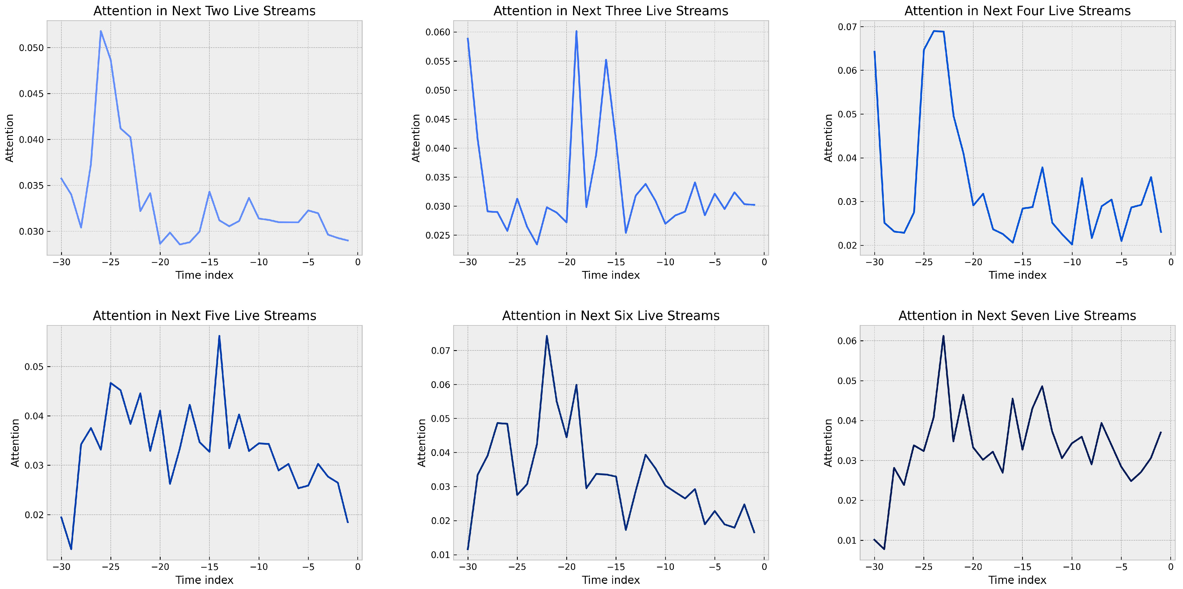
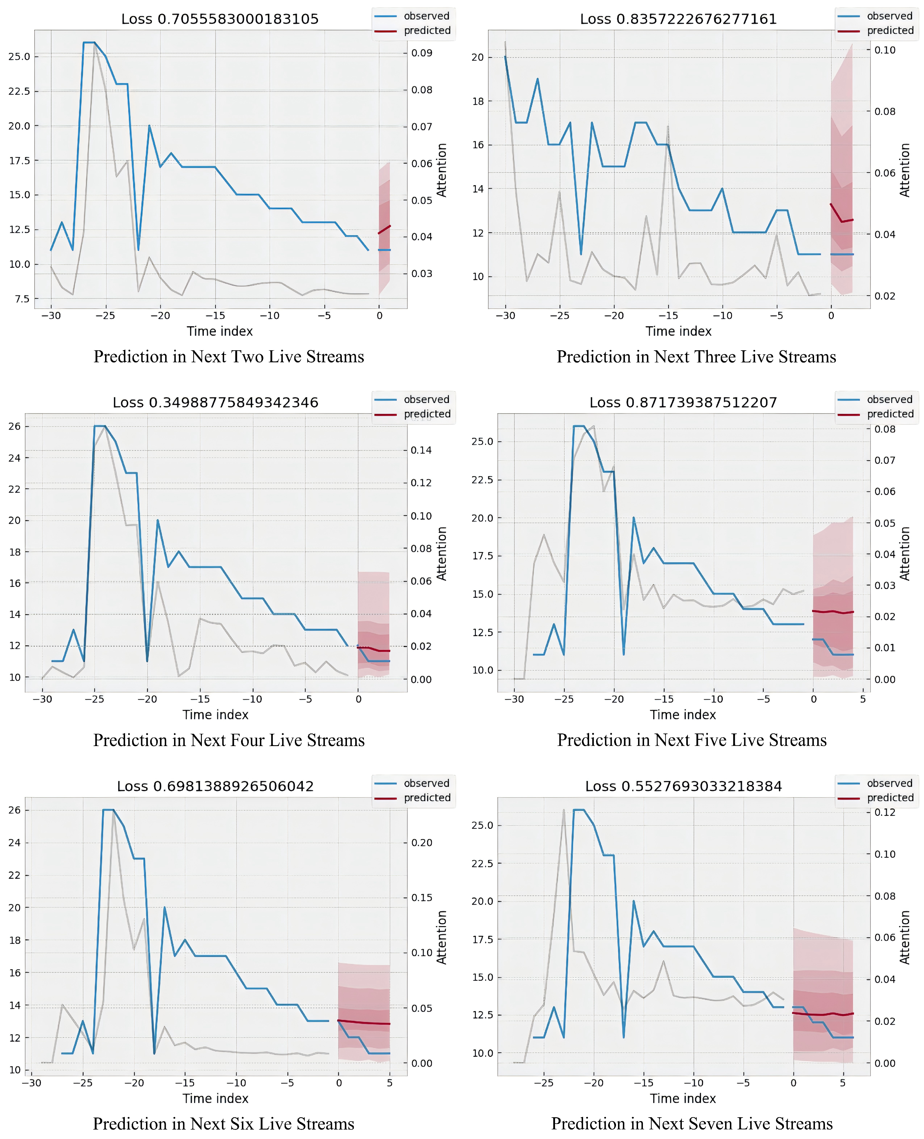
This section explores the application of the Temporal Fusion Transformer (TFT) model in predicting UK cross-border e-commerce live sales. The study reveals how the TFT model captures key patterns in sales data from multiple dimensions by analyzing the attention mechanism, static variables, long-term and short-term memory capabilities, and the importance of various features in the model. Through this analysis, the study provides feasible suggestions for cross-border e-commerce companies in optimizing inventory management and formulating precision marketing strategies.

4.4.1. Attention

Figure 5 illustrates the distribution of attention weights across forecast horizons (2–7 periods), highlighting the TFT model’s adaptive focus on historical time points. Key findings include:

• Short-term forecast (2–3 steps): The model places more emphasis on older historical data (−30 to −25 periods) to capture long-term trends that are critical for short-term forecasts. The focus on recent data is reduced, reflecting the model’s reliance on established patterns rather than immediate fluctuations.
• Medium-term forecast (4–5 steps): The attention weights are more evenly distributed, peaking between −15 and −10 periods while remaining sensitive to earlier trends. This balance suggests that the model considers short-term fluctuations and broader sales trends.
• Long-term forecast (steps 6–7): The shift in focus to the −25 to −20 period shows that the model focuses on medium-term trends and reduces reliance on recent data. This highlights the model’s ability to capture cyclical patterns and maintain long-term sales forecasts.

Figure 5. Temporal Fusion Transformer architecture for forecasting cross-border e-commerce sales (The x-axis represents the temporal dimension, depicting a time series. The y-axis displays independent variables influencing UK cross-border live-streaming e-commerce sales, including historical sales, KOL characteristics, seasonality, and weekend/holiday effects).

Figure 5. Temporal Fusion Transformer architecture for forecasting cross-border e-commerce sales (The x-axis represents the temporal dimension, depicting a time series. The y-axis displays independent variables influencing UK cross-border live-streaming e-commerce sales, including historical sales, KOL characteristics, seasonality, and weekend/holiday effects).

By dynamically adjusting attention, the TFT model enhances interpretability and provides actionable insights for optimizing sales strategies.

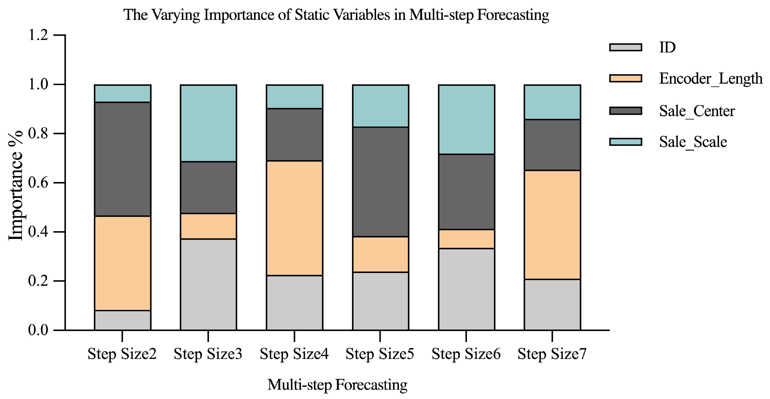
4.4.2. Importance of Static Variables

Figure 6 illustrates the importance of various static features for predicting UK cross-border e-commerce live-streaming sales using a Temporal Fusion Transformer (TFT) model with different forecast horizons. The key findings of the static feature importance analysis are as follows:

• Product Category (ID): The importance of this feature varies across different forecast horizons. A higher value indicates a stronger influence on the prediction.
• Encoder Length (Encoder_Length): The length of the input time series significantly impacts prediction accuracy. The varying importance across different forecast horizons suggests that the relevance of historical data changes with the prediction time frame.
• Sales Center (Sale_Center): Representing the central tendency of historical sales data (e.g., mean or median), this feature’s importance fluctuates, indicating its varying contribution to predictions at different horizons.
• Sales Scale (Sale_Scale): This feature reflects the range or dispersion of historical sales data and its influence on the target variable prediction.

In short-term predictions (2–3 steps), the sales center and encoder length are the most influential features, suggesting that recent sales trends and input sequence length are crucial for accurate short-term forecasting.

For medium-term predictions (4–5 steps), the product category becomes more critical, along with the sales scale. Understanding product-specific trends and historical sales variability is essential for medium-term forecasting.

In long-term predictions (6–7 steps), the importance of encoder length shifts significantly, highlighting the complex and dynamic role of historical information in long-term forecasting.

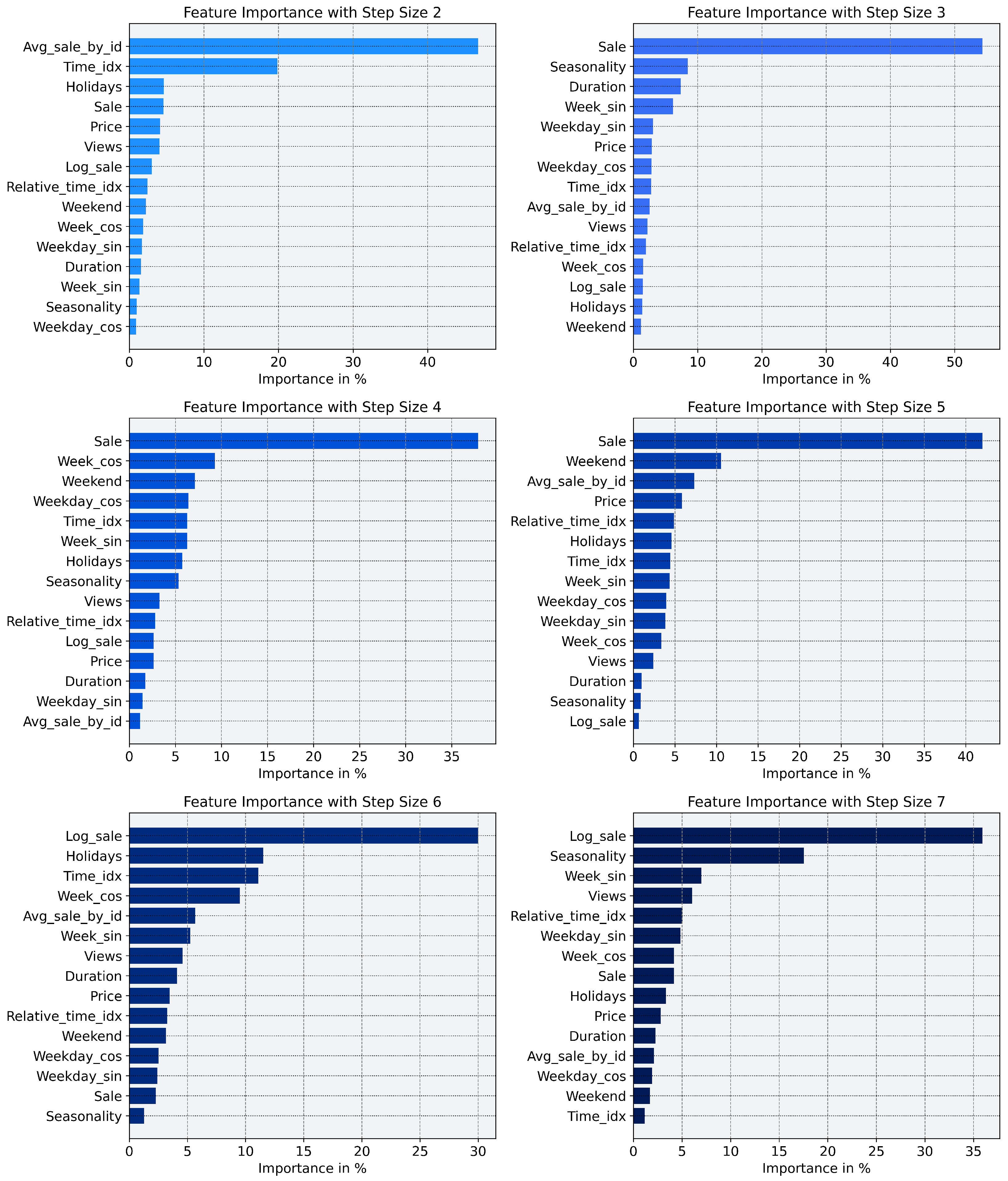
4.4.3. Dynamic Feature Weights in Multi-Horizon Forecasting

By training on live broadcast data from UK cross-border e-commerce, we predicted the sales value for the following two to seven live broadcasts using the enhanced Temporal Fusion Transformer (TFT) model. We analyzed how the importance of each feature changed at different prediction steps. This study aims to deeply reveal the model’s ability to explain each feature in different prediction time ranges. Specifically,

Table 4. Contributions of different features at varying prediction steps.

Variables	Short-Term Forecast		Medium-Term Forecast		Long-Term Forecast
	Size 2	Size 3	Size 4	Size 5	Size 6	Size 7
Sale	4.58%	54.30%	37.87%	41.99%	2.27%	4.17%
Log_sale	3.02%	1.46%	2.62%	0.66%	30.00%	35.90%
Avg_sale_by_id	46.77%	2.55%	1.18%	7.32%	5.67%	2.12%
Time_idx	19.84%	2.77%	6.28%	4.43%	11.08%	1.15%
Relative_Time_idx	2.42%	1.93%	2.82%	4.87%	3.27%	5.04%
Weekday_cos	0.92%	2.82%	6.42%	3.93%	2.51%	1.91%
Weekday_sin	1.70%	3.05%	1.44%	3.85%	2.41%	4.83%
Week_cos	1.86%	1.50%	9.27%	3.34%	9.49%	4.17%
Week_sin	1.36%	6.17%	6.27%	4.37%	5.24%	7.00%
Seasonality	0.98%	8.43%	5.34%	0.88%	1.26%	17.56%
Holidays	4.62%	1.39%	5.75%	4.59%	11.50%	3.33%
Weekend	2.21%	1.17%	7.11%	10.53%	3.14%	1.70%
Price	4.12%	2.88%	2.61%	5.84%	3.47%	2.81%
Duration	1.56%	7.38%	1.73%	1.00%	4.11%	2.29%
Views	4.03%	2.21%	3.27%	2.40%	4.57%	6.03%

and Figure 7 illustrate the dynamic evolution of the importance of these features.

(1) Short-Term Forecasting (Step Length 2–3)

For short-term forecasting (step length 2–3), the feature average sales by product ID (Avg_sale_by_id) holds the highest weight (46.77% at step 2), suggesting that the historical average sales of products are crucial in predicting immediate future sales. As the prediction step increases from 2 to 3, the weight of original sales (Sale) increases significantly (jumping from a low level to 54.30%), indicating that historical sales data plays a key role in predicting the sales of the following three live broadcasts. The shift indicates that historical sales data becomes more influential as the forecast horizon extends. Furthermore, the weights of live broadcast duration (Duration), periodic features (Week_sin), and seasonality (Seasonality) gradually increase, signifying that time-related factors gain greater importance as the forecast horizon grows.

(2) Medium-Term Forecasting (Step Length 4–5)

The weight distribution shifts notably in medium-term forecasting (step length 4–5). While historical sales data (original sales) still dominate (37.87% and 41.99% at steps 4 and 5, respectively), their relative importance decreases compared to short-term forecasting. At step 4, the time index (Time_idx) becomes more prominent, underlining the continued relevance of sequential information in medium-term predictions. At step 5, the weight of the weekend effect (Weekend) increases substantially, indicating that the model begins to account more heavily for weekend-driven variations in sales when predicting future live stream sales.

(3) Long-Term Forecasting (Step Length 6–7)

For long-term forecasting (step length 6–7), the model’s reliance shifts towards smoothed sales data (Log_sale) and seasonal features (Seasonality), which play a more significant role in capturing long-term trends. At step 6, the weight of log of sales (Log_sale) rises to 30.00%, reflecting that smoothed sales data provides a more stable signal for predicting long-term trends. Additionally, the weight of the holiday effect (Holidays) increases, suggesting that holidays have a significant impact on long-term sales patterns. By step 7, the weight of log of sales further increases to 35.90%, while seasonality reaches 17.56%, highlighting the growing importance of seasonal patterns.

4.4.4. Importance of Different Features

This section discusses the importance of various features in forecasting UK cross-border e-commerce product demand, mainly focusing on live-streaming sales, temporal, weekend, holiday effects, and KOL delivery features.

(1) Live-streaming Sales Features

Original Sales (Sale): As the raw historical sales data, ’Original Sales’ captures the underlying sales trend. This feature showed the highest importance for medium-term forecasting (3 and 5 steps), with scores of 54.30% and 41.99%, respectively. This suggests that historical sales data plays a dominant role in medium-term predictions.

Logarithmic Sales (Log_sale): By applying a logarithmic transformation, ’Log_sale’ smooths fluctuations and reduces the impact of extreme values. It showed higher importance in long-term forecasting (6 and 7 steps), with scores of 30.00% and 35.90%, respectively, suggesting that smoothed data provides more stable signals for long-term predictions.

Average Sales by Product ID (Avg_sale_by_id): Reflecting the heterogeneity in sales levels across products, ’Avg_sale_by_id’ had a significant impact on both short-term (2-step, 46.77%) and medium-term (5-step, 7.32%) forecasting, indicating that product-level sales averages are valuable for predicting demand in these horizons.

(2) KOL Delivery Features

Among KOL indicators, price and number of viewers are more important than duration. KOL and brand bargaining power and ability to attract viewers can more significantly impact live sales.

Price (Price): Product price information indicates price fluctuations’ potential impact on sales. In step 5 (mid-term forecast), the importance of price is relatively high (5.84%), suggesting that price fluctuations may be a key influencing factor in the mid-term forecast.

Duration (Duration): Indicates the duration of each live broadcast, reflecting the audience’s attention to the product. In steps 3 and 6 (mid-term forecast), the importance of live broadcast duration is relatively high (7.38% and 4.11%), indicating that a longer live broadcast time may enhance the audience’s willingness to buy.

Views (Views): This indicator directly affects sales by indicating the number of viewers watching the live broadcast. In the step length (short-term and long-term forecasts), the average weight of the number of viewers is 3.12% and 5.3%, respectively, indicating that the number of viewers is more important in the short-term and long-term forecasts. The average weight in the medium-term forecast is 2.835%, and the impact is relatively weak.

(3) Temporal Features

Time Index (Time_idx): This feature helps capture sequential changes in the time series. Its importance was higher for short-term forecasting (2-step, 19.84%), indicating a stronger dependence on time order in short-term predictions.

Relative Time Index (Relative_Time_idx): The relative position of the current time in the sequence was most impactful in longer forecasting horizons (5 and 7 steps, 4.87% and 5.04%, respectively), suggesting its greater relevance for long-term predictions.

Cyclic Features (Weekday_cos, Weekday_sin, Week_cos, Week_sin): These features capture weekly and monthly cyclical patterns. For medium-term forecasting (4-step), the importance of weekly cycles (Week_cos, Week_sin) increased significantly (9.27% and 6.27%), suggesting that cyclical fluctuations are more pronounced in medium-term sales fluctuations.

Seasonality (Seasonality): The seasonality feature, which captures seasonal patterns in sales, showed lower importance in short-term forecasting. However, in long-term forecasting (7-step), its importance rose significantly (17.56% ), indicating seasonal effects’ growing relevance over extended time horizons.

(4) Weekend and Holiday Effects

Holiday Effect (Holidays): This captures the influence of holidays on sales. The significantly increased weight of the holiday effect (6-step, 11.50%) in Step 6 underscores the importance of holidays in accurately forecasting long-term sales.

Weekend Effect (Weekend): The weekend effect showed higher importance in medium-term forecasting (5-step, 10.53%), suggesting that weekends have a more substantial influence on sales during medium-term prediction.

4.5. Commercial Applications of Model Interpretability

The feature importance analysis leveraging the Temporal Fusion Transformer (TFT) provides actionable decision support for cross-border live-streaming e-commerce operations in the United Kingdom. The dynamic variations in feature contributions across distinct forecast horizons enable targeted optimization of critical business processes through the following approaches:

4.5.1. Spatiotemporal Optimization of Marketing Budgets

(1) Temporal dimension

When the model exhibits uniform attention to historical data from t-15 to t-10 in mid-term forecasts (Figure 5), this indicates sustained impacts of current marketing activities on sales 4–5 weeks post-campaign. We recommend allocating 40% of the budget to content marketing with long-tail effects (e.g., product tutorial videos) rather than solely focusing on live-streaming ads for immediate conversions.

(2) Spatial dimension

Fluctuations in feature importance for static variables ID and $\mathit{Sale\_Scale}$ (increasing by 29.07% and 24.19%, respectively, at prediction horizon 3) suggest differentiated regional allocation strategies. For product categories sensitive to encoder lengths, targeted budget allocations should be increased by 15%–20% in European markets with robust historical sales data while adopting conservative exploratory testing in emerging markets.

4.5.2. Three-Tier Responsive Mechanism for Dynamic Inventory Management

(1) Short-term forecasting (Horizon = 2–3):

With high-weight historical data features (approximately 55% contribution), it is recommended to implement an agile replenishment mechanism (When the forecast horizon is h = 2, the percentage contributions to the predictive model are as follows: original sales ($Sale$) account for 4.58%, the logarithm of sales ($\mathit{Log\_sale}$) contribute 3.02%, and average sales by product ID ($\mathit{Avg\_sale\_by\_id}$) dominate with 46.77%, yielding a cumulative contribution of 54.36%. A similar analytical framework applies to predictions with a forecast horizon of h = 3). From an inventory management perspective, when the model detects a significant surge in $\mathit{Avg\_sale\_by\_id}$ (average sales volume by product ID) for specific SKUs, an automated procurement system should be activated to elevate safety stock levels to 130–150% of forecasted demand values. This adaptive protocol effectively addresses sudden sales surges during peak consumption periods while maintaining optimal inventory turnover efficiency.

(2) Mid-term forecasting (horizon = 4–5):

The Weekend Effect and Price Sensitivity demonstrate elevated contribution rates of 10.53% and 5.84%, respectively, necessitating the establishment of promotion-driven elastic inventory reserves. Specifically, when the forecast horizon encompasses weekends, regional warehouse stock levels for associated merchandise should be augmented two weeks in advance, accompanied by the implementation of dynamic capacity agreements with logistics providers.

(3) Long-term forecasting (horizon = 6–7):

The cumulative contribution of seasonal patterns and logarithmic sales characteristics reaches 53.46% (h = 7), triggering strategic procurement decisions:

• Execute capacity framework agreements aligned with long-term $\mathit{Log\_sale}$ trends while adjusting overseas warehouse baseline inventory through seasonality indices;
• Initiate prelaunch phases 6–7 weeks preceding major promotional seasons (e.g., Christmas/Black Friday), with inventory replenishment timelines determined through backward scheduling from customs clearance cycles.

4.5.3. Feedback Control System for Real-Time Decision-Making

(1) Short-term forecasting (Horizon 2–3):

During product cold-start phases, sales operations should prioritize historical analogues from comparable merchandise to rapidly establish baseline expectations. Marketing resources should be strategically allocated to historically top-performing homogeneous products, with live-streaming scripts emphasizing “proven sales performance” messaging frameworks.

(2) Mid-term forecasting (horizon = 4–5):

A dynamic pricing model should be constructed by integrating mid-term price feature weights (5.84%) with historical price fluctuation sensitivity. Given the pronounced Weekend Effect (7–11% impact magnitude at Horizon = 4–5), time-limited promotions should be concentrated from Thursday to Saturday, coupled with proactive adjustments to cross-border logistics capacity in anticipation of weekend order surges.

(3) Long-term forecasting (horizon = 6–7):

The escalating significance of seasonal patterns necessitates real-time optimization of live-stream product selection based on seasonal demand fluctuations.

Through this implementation framework, the Temporal Fusion Transformer (TFT) model not only generates predictive outputs but also establishes a closed-loop “forecasting-attribution-decision” system via its interpretability modules. Enterprises should operationalize attention weight distributions as key metrics in strategic dashboards, while embedding feature importance rankings into automated decision pipelines, thereby achieving effective transformation of predictive analytics into measurable business value.

5. Conclusions

This study draws the following primary conclusions based on the predictive and interpretative analysis of cross-border e-commerce live-streaming sales on TikTok in the UK using the Temporal Fusion Transformer (TFT) model.

(1) Performance Superiority of the TFT Model: The Temporal Fusion Transformer (TFT) model demonstrates significant performance superiority in forecasting cross-border e-commerce sales for live-streaming commerce in the UK.Experimental results reveal that, across all prediction horizons spanning two to seven subsequent live-streaming sessions, the TFT model consistently achieves lower Mean Absolute Error (MAE), Root Mean Squared Error (RMSE), and Mean Squared Error (MSE), with respective ranges of $[2.323,2.949]$, $[2.571,3.650]$, and $[6.611,13.320]$, outperforming conventional machine learning approaches including Long Short-Term Memory networks (LSTM), Graph Neural Networks (GNN), and Convolutional Neural Networks (CNN). The prediction effect of the machine learning model is much better than that of the ARIMA model. The above findings are consistent with previous research [38], further validating the feasibility and rationality of prioritizing the TFT model in cross-border e-commerce scenarios.

(2) Dynamic Feature Importance Analysis: Compared to traditional ARIMA models, TFT models demonstrate stronger interpretability in time series forecasting. This paper reveals the dynamic impact of different feature variables on prediction results through a dynamic forecasting analysis of cross-border e-commerce live-streaming sales on TikTok in the UK.

• Static Features: The importance of static features varies significantly in different forecast periods. This result inspires subsequent research. The weight changes of static features in different prediction periods should be fully considered when constructing a cross-border e-commerce live broadcast prediction model.
• Sales Features: Historical sales volume is crucial in forecasting. However, this paper further examines the significant role of historical sales data in predicting the entire life cycle of product sales, compared to existing research [43,44].
• KOL Features: In contrast, the duration of live streams has a weaker impact on sales forecasting because consumers pay more attention to the quality and interactivity of the live stream content. This study further enriches the theoretical explanation of the spillover effects of KOLs on live marketing [45,49], revealing the critical role of KOLs from a new perspective of the product marketing cycle and utilizing the interpretability of TFT models to make the mechanism of influence of KOLs more straightforward.
• Time-Series Features: Time index (Time_idx) and periodic features (e.g., Week_sin, Week_cos) contribute significantly to the prediction of medium and short-term sales, indicating that periodic factors have a significant impact in the short term. In contrast, seasonal features and relative time index become significantly more important in long-term forecasting, showing the key role of seasonal variations and long-term trends in long-term sales forecasting. This conclusion further verifies the importance of time features (such as seasonal factors) in sales forecasting [51,52,54].

(3) Comprehensive Interpretation of the Product Marketing Cycle: This article introduces the concepts of short-term forecast, medium-term forecast, and long-term forecast, thus constructing a more comprehensive forecast system for UK cross-border e-commerce live-streaming sales. The research shows that:

• Short-term forecasting (step size = 2 to 3): The model primarily relies on static features such as the average product ID sales and the sequential time series information.
• Medium-term forecasting (step size = 4 to 5): The model depends more on the volatility of historical sales data, periodic features, and the impact of holidays and weekends.
• Long-term forecasting (step size = 6 to 7): In the long-term forecast, the importance of smoothed sales data (Log_sale) and seasonal features increases significantly, indicating that the model relies more on stable signals in capturing long-term trends.

(4) Interpretability of Macroeconomic Trends: Sales volume shows a downward trend from the overall trend, which may be related to the changes in the cross-border e-commerce trade environment after Brexit. This shows that the TFT model not only shows a high degree of accuracy in sales volume forecasting but also has the potential to analyze the macroeconomic background behind sales volume.

Overall, this paper has demonstrated the significant advantages of the Temporal Fusion Transformer (TFT) model in forecasting cross-border e-commerce live-streaming sales in the UK. Through multidimensional feature analysis and model performance evaluation, this paper has proven the effectiveness of the TFT model in improving sales forecasting accuracy and interpretability. This provides a theoretical basis for formulating future intelligent sales strategies and offers an efficient and convenient technical solution for cross-border e-commerce forecasting in other countries or regions through the reproducibility of this model and code, thus playing a positive role in enterprise inventory management and risk control.

6. Limitations and Future Research

6.1. Limitations

This paper has made progress in enhancing the application capabilities of the Temporal Fusion Transformer (TFT) model in the product sales cycle and improved the live broadcast sales prediction system framework, thereby providing a more effective solution for corporate live broadcast sales decisions. However, some shortcomings still give room for future research optimization. Future research can build a more comprehensive measurement framework to comprehensively evaluate the influence of KOLs on sales based on multidimensional characteristics. This paper does not conduct an in-depth analysis of regional characteristic variables. This may limit the applicability of the research conclusions in cross-border e-commerce live broadcast scenarios in other regions and fail to fully consider the potential impact of regional differences on sales forecasts.

6.2. Future Directions

6.2.1. Enhanced Modeling of KOL Features

Future studies should incorporate a broader range of KOL attributes to improve interpretability and prediction accuracy. For example, a composite KOL influence score can be constructed based on metrics like engagement rate, follower conversion rate, and live-streaming frequency, which could offer a more holistic view of KOL effectiveness. Additionally, learning algorithms could be employed to predict conversion rates using these expanded features.

6.2.2. Integration of Regional Features

Divergent consumer behaviors, regulatory frameworks, and market competition landscapes across regions (e.g., other European countries, North America, and Southeast Asia) may differentially impact cross-border live-stream sales performance. Subsequent research could develop region-specific forecasting models based on multi-regional datasets to analyze market heterogeneity factors, while exploring transfer learning methodologies to improve model adaptability in emerging markets. Additionally, investigations into cross-market interdependencies—such as whether live-stream sales trends in one market could provide effective prior knowledge for others—would be valuable for optimizing transnational prediction frameworks. This line of inquiry could further examine how inter-market influences might inform predictive methodologies through shared temporal patterns or demand spillover effects.

6.2.3. Integration of Category Features

Current research primarily focuses on forecasting overall cross-border e-commerce live-stream sales, while products across different categories may exhibit distinct sales patterns and temporal characteristics. For instance, categories such as fast-moving consumer goods, electronics, and apparel could be influenced by varying seasonal effects, promotional campaigns, and market demand fluctuations. Future studies should therefore establish multi-category benchmark datasets and integrate Temporal Fusion Transformer (TFT) models or other deep learning approaches to investigate the generalization capability and applicability of cross-category sales prediction, thereby enhancing the practical utility of forecasting models.

6.2.4. Extension to Multimodal Data Integration

Incorporating multimodal data processing capabilities could significantly enhance the model’s applicability to live-streaming scenarios. For instance, Convolutional Neural Networks (CNNs) could process visual data to evaluate product displays and brand elements, while Recurrent Neural Networks (RNNs) could analyze audio features to assess presentation styles. Integrating these modalities with time-series data would enable the model to identify latent factors influencing sales, thereby improving prediction accuracy and decision-making utility.

References

1. Zhang, X.; Zha, X.; Dan, B.; Liu, Y.; Sui, R. Logistics Mode Selection and Information Sharing in a Cross-Border e-Commerce Supply Chain with Competition. Eur. J. Oper. Res. 2024, 314, 136–151. [Google Scholar] [CrossRef]
2. Chen, S.; Ke, S.; Han, S.; Gupta, S.; Sivarajah, U. Which Product Description Phrases Affect Sales Forecasting? An Explainable AI Framework by Integrating WaveNet Neural Network Models with Multiple Regression. Decis. Support Syst. 2024, 176, 114065. [Google Scholar] [CrossRef]
3. APAC Regulatory & Legal Salary Guide. Available online: https://www.larsonmaddox.com/regulatory-and-legal-salary-guide-compensation-benchmarking-in-key-industries-across-APAC (accessed on 1 January 2024).
4. Derindag, O.F.; Yasar, Z.R.; Aslan, C.; Parmaksiz, S. Analyzing the differential effects of COVID-19 on export flows: A focus on customs procedures. Empirica 2024, 51, 977–1000. [Google Scholar] [CrossRef]
5. Aslan, C.; Derindag, O.F.; Parmaksiz, S. Effects of cross-border E-commerce customs declaration ceiling increase on export performance under COVID-19 conditions. Kybernetes 2024, 53, 3348–3364. [Google Scholar] [CrossRef]
6. Roscoe, S.; Skipworth, H.; Aktas, E.; Habib, F. Managing Supply Chain Uncertainty Arising from Geopolitical Disruptions: Evidence from the Pharmaceutical Industry and Brexit. Int. J. Oper. Prod. Manag. 2020, 40, 1499–1529. [Google Scholar] [CrossRef]
7. Queiroz, M.M.; Fosso Wamba, S.; Chiappetta Jabbour, C.J.; Machado, M.C. Supply Chain Resilience in the UK during the Coronavirus Pandemic: A Resource Orchestration Perspective. Int. J. Prod. Econ. 2022, 245, 108405. [Google Scholar] [CrossRef]
8. Ma, J.; Chen, J.; Zhang, G.; Chen, S. Online Opinion Leadership Styles and Purchase Intention in Livestreaming E-Commerce. Serv. Ind. J. 2024, 1–27. [Google Scholar] [CrossRef]
9. Pappas, N. UK Outbound Travel and Brexit Complexity. Tour. Manag. 2019, 72, 12–22. [Google Scholar] [CrossRef]
10. Trade, Migration and Brexit. Available online: https://ukandeu.ac.uk/trade-migration-and-brexit/ (accessed on 25 October 2022).
11. Qian, L. The Global Imperative: Chinese Cross-Border E-Commerce and Its Political-Economic Implications in a Deglobalising World. Asian Stud. Rev. 2024, 48, 828–846. [Google Scholar] [CrossRef]
12. Xu, Y.; Zeng, K.; Guo, J.; Li, X.; Dong, L.; Jiang, W. Whether Live Streaming Has a Better Performance? An Examination of Product Presentation Modes on Cross-Border E-Commerce Platform. Int. J. Hum.-Comput. Interact. 2023, 41, 69–84. [Google Scholar] [CrossRef]
13. Gong, H.; Zhao, M.; Ren, J.; Hao, Z. Live Streaming Strategy under Multi-Channel Sales of the Online Retailer. Electron. Commer. Res. Appl. 2022, 55, 101184. [Google Scholar] [CrossRef]
14. Zhang, W.; Liu, C.; Ming, L.; Cheng, Y. The sales impacts of traffic acquisition promotion in live-streaming commerce. Prod. Oper. Manag. 2022, 10591478231224938. [Google Scholar] [CrossRef]
15. Xu, W.; Cao, Y.; Chen, R. A multimodal analytics framework for product sales prediction with the reputation of anchors in live streaming e-commerce. Decis. Support Syst. 2024, 177, 114104. [Google Scholar] [CrossRef]
16. Lu, B.; Chen, Z. Live streaming commerce and consumers’ purchase intention: An uncertainty reduction perspective. Inf. Manag. 2021, 58, 103509. [Google Scholar] [CrossRef]
17. Frontiers | How Live Streaming Features Impact Consumers’ Purchase Intention in the Context of Cross-Border E-Commerce? A Research Based on SOR Theory. Available online: https://www.frontiersin.org/journals/psychology/articles/10.3389/fpsyg.2021.767876/full (accessed on 4 January 2025).
18. Alabdulrazzaq, H.; Alenezi, M.N.; Rawajfih, Y.; Alghannam, B.A.; Al-Hassan, A.A.; Al-Anzi, F.S. On the Accuracy of ARIMA Based Prediction of COVID-19 Spread. Results Phys. 2021, 27, 104509. [Google Scholar] [CrossRef]
19. Wang, X.; Kang, Y.; Hyndman, R.J.; Li, F. Distributed ARIMA models for ultra-long time series. Int. J. Forecast. 2023, 39, 1163–1184. [Google Scholar] [CrossRef]
20. Lu, S. Research on GDP forecast analysis combining BP neural network and ARIMA model. Comput. Intell. Neurosci. 2021, 2021, 1026978. [Google Scholar] [CrossRef]
21. Kim, S.; Choi, C.Y.; Shahandashti, M.; Ryu, K.R. Improving accuracy in predicting city-level construction cost indices by combining linear ARIMA and nonlinear ANNs. J. Manag. Eng. 2022, 38, 04021093. [Google Scholar] [CrossRef]
22. He, Q.Q.; Wu, C.; Si, Y.W. LSTM with particle swarm optimization for sales forecasting. Electron. Commer. Res. Appl. 2022, 51, 101118. [Google Scholar] [CrossRef]
23. Wu, H. Predicting e-commerce product prices through the integration of variational mode decomposition and deep neural networks. PeerJ Comput. Sci. 2024, 10, e2353. [Google Scholar] [CrossRef]
24. Lim, B.; Arık, S.Ö.; Loeff, N.; Pfister, T. Temporal fusion transformers for interpretable multi-horizon time series forecasting. Int. J. Forecast. 2021, 37, 1748–1764. [Google Scholar] [CrossRef]
25. Wang, Y.; Jia, F.; Schoenherr, T.; Chen, L. Cross-border e-commerce firms as supply chain integrators: The management of three flows. Ind. Mark. Manag. 2020, 89, 72–88. [Google Scholar] [CrossRef]
26. Lin, Q.; Jia, N.; Chen, L.; Zhong, S.; Yang, Y.; Gao, T. A two-stage prediction model based on behavior mining in livestream e-commerce. Decis. Support Syst. 2023, 174, 114013. [Google Scholar] [CrossRef]
27. Wu, H.; Qiao, Y.; Luo, C. Cross-border e-commerce, trade digitisation and enterprise export resilience. Financ. Res. Lett. 2024, 65, 105513. [Google Scholar] [CrossRef]
28. Koutsandreas, D.; Spiliotis, E.; Petropoulos, F.; Assimakopoulos, V. On the selection of forecasting accuracy measures. J. Oper. Res. Soc. 2022, 73, 937–954. [Google Scholar] [CrossRef]
29. Muthukalyani, A.R. Unlocking accurate demand forecasting in retail supply chains with AI-driven predictive analytics. Inf. Technol. Manag. 2023, 14, 48–57. [Google Scholar]
30. Cheba, K.; Kiba-Janiak, M.; Baraniecka, A.; Kołakowski, T. Impact of external factors on e-commerce market in cities and its implications on environment. Sustain. Cities Soc. 2021, 72, 103032. [Google Scholar] [CrossRef]
31. Daniel, C.; Hernandez, T. What retail apocalypse? A Delphi forecast of commercial space demand in the Toronto region. J. Retail. Consum. Serv. 2024, 77, 103670. [Google Scholar] [CrossRef]
32. Cai, W.; Song, Y.; Wei, Z. Multimodal Data Guided Spatial Feature Fusion and Grouping Strategy for E-Commerce Commodity Demand Forecasting. Mob. Inf. Syst. 2021, 2021, 5568208. [Google Scholar] [CrossRef]
33. Li, Z.; Zhang, N. Short-Term Demand Forecast of E-Commerce Platform Based on ConvLSTM Network. Comput. Intell. Neurosci. 2022, 2022, 5227829. [Google Scholar] [CrossRef]
34. Zhang, B.; Tseng, M.L.; Qi, L.; Guo, Y.; Wang, C.H. A comparative online sales forecasting analysis: Data mining techniques. Comput. Ind. Eng. 2023, 176, 108935. [Google Scholar] [CrossRef]
35. Suryawan, I.G.T.; Putra, I.K.N.; Meliana, P.M.; Sudipa, I.G.I. Performance Comparison of ARIMA, LSTM, and Prophet Methods in Sales Forecasting. Sink. J. Tek. Inform. 2024, 8, 2410–2421. [Google Scholar] [CrossRef]
36. Dhankhar, S.; Dhankhar, N.; Sandhu, V.; Mehla, S. Forecasting Electric Vehicle Sales with ARIMA and Exponential Smoothing Method: The Case of India. Transport. Dev. Econ. 2024, 10, 32. [Google Scholar] [CrossRef]
37. Elalem, Y.K.; Maier, S.; Seifert, R.W. A machine learning-based framework for forecasting sales of new products with short life cycles using deep neural networks. Int. J. Forecast. 2023, 39, 1874–1894. [Google Scholar] [CrossRef]
38. Xie, L.; Liu, J.; Wang, W. Predicting sales and cross-border e-commerce supply chain management using artificial neural networks and the Capuchin search algorithm. Sci. Rep. 2024, 14, 13297. [Google Scholar] [CrossRef]
39. Chen, Y.; Xie, X.; Pei, Z.; Yi, W.; Wang, C.; Zhang, W.; Ji, Z. Development of a Time Series E-Commerce Sales Prediction Method for Short-Shelf-Life Products Using GRU-LightGBM. Appl. Sci. 2024, 14, 866. [Google Scholar] [CrossRef]
40. Bhatt, S.; Ghazanfar, M.; Amirhosseini, M. Machine learning based cryptocurrency price prediction using historical data and social media sentiment. Comput. Sci. Inf. Technol. 2023, 13, 1–11. [Google Scholar]
41. Pongdatu, G.A.N.; Putra, Y.H. Seasonal time series forecasting using sarima and holt winter’s exponential smoothing. IOP Conf. Ser. Mater. Sci. Eng. 2018, 407, 012153. [Google Scholar] [CrossRef]
42. Zhuang, Q.; Zhang, X.; Wang, P.; Deng, B.; Pan, H. A neural network model for China B2C e-commerce sales forecast based on promotional factors and historical data. In Proceedings of the 2019 International Conference on Economic Management and Model Engineering (ICEMME), Malacca, Malaysia, 6–8 December 2019; pp. 307–312. [Google Scholar]
43. Liu, J.; Liu, C.; Zhang, L.; Xu, Y. Research on sales information prediction system of e-commerce enterprises based on time series model. Inf. Syst. e-Bus. Manag. 2020, 18, 823–836. [Google Scholar] [CrossRef]
44. Chen, J.; Lan, Y.C.; Chang, Y.W. Consumer behaviour in cross-border e-commerce: Systematic literature review and future research agenda. Int. J. Consum. Stud. 2023, 47, 2609–2669. [Google Scholar] [CrossRef]
45. He, P.; Shang, Q.; Pedrycz, W.; Chen, Z.S. Short video creation and traffic investment decision in social e-commerce platforms. Omega 2024, 128, 103129. [Google Scholar] [CrossRef]
46. Niu, B.; Yu, X.; Dong, J. Could AI livestream perform better than KOL in cross-border operations? Transp. Res. Part E Logist. Transp. Rev. 2023, 174, 103130. [Google Scholar] [CrossRef]
47. Zhang, H.; Sui, R.; Zha, X. The key opinion leader introduction and pricing strategy for live streaming e-commerce platforms considering the impact of network effects. J. Retail. Consum. Serv. 2025, 82, 104077. [Google Scholar] [CrossRef]
48. He, W.; Jin, C. A study on the influence of the characteristics of key opinion leaders on consumers’ purchase intention in live streaming commerce: Based on dual-systems theory. Electron. Commer. Res. 2024, 24, 1235–1265. [Google Scholar] [CrossRef]
49. Lin, X.; Gui, L.; Lu, Y. Managing sales via livestream commerce: Implications of price negotiation and consumer price search. Prod. Oper. Manag. 2024, 10591478231224930. [Google Scholar] [CrossRef]
50. Xiong, L.; Cho, V.; Law, K.M.Y.; Lam, L. A study of KOL effectiveness on brand image of skincare products. Enterp. Inf. Syst. 2021, 15, 1483–1500. [Google Scholar] [CrossRef]
51. Moorthi, K.; Srihari, K.; Karthik, S. Improving business process by predicting customer needs based on seasonal analysis: The role of big data in e-commerce. Int. J. Bus. Excell. 2020, 20, 561–574. [Google Scholar] [CrossRef]
52. Liu, X.; Zhou, Y.W.; Shen, Y.; Ge, C.; Jiang, J. Zooming in the impacts of merchants’ participation in transformation from online flash sale to mixed sale e-commerce platform. Inf. Manag. 2021, 58, 103409. [Google Scholar] [CrossRef]
53. Fathalla, A.; Salah, A.; Li, K.; Li, K.; Francesco, P. Deep end-to-end learning for price prediction of second-hand items. Knowl. Inf. Syst. 2020, 62, 4541–4568. [Google Scholar] [CrossRef]
54. Kharfan, M.; Chan, V.W.K.; Firdolas Efendigil, T. A data-driven forecasting approach for newly launched seasonal products by leveraging machine-learning approaches. Ann. Oper. Res. 2021, 303, 159–174. [Google Scholar] [CrossRef]
55. Zhao, Y. Research on E-Commerce Retail Demand Forecasting Based on SARIMA Model and K-means Clustering Algorithm. Acad. J. Sci. Technol. 2024, 10, 226–231. [Google Scholar] [CrossRef]
56. Tran, D.T.; Huh, J.H. Forecast of seasonal consumption behavior of consumers and privacy-preserving data mining with new S-Apriori algorithm. J. Supercomput. 2023, 79, 12691–12736. [Google Scholar] [CrossRef]
57. Deng, L.; Ye, Q.; Xu, D.; Sun, F. The “holiday effect” in consumer satisfaction: Evidence from review ratings. Inf. Manag. 2023, 60, 103863. [Google Scholar] [CrossRef]
58. Bir, C.L.; Widmar, N.J.O.; Davis, M.K.; Erasmus, M.A.; Zuelly, S. Willingness to pay for whole turkey attributes during Thanksgiving holiday shopping in the United States. Poult. Sci. 2020, 99, 2798–2810. [Google Scholar] [CrossRef]
59. Zane, D.M.; Reczek, R.W.; Haws, K.L. Promoting pi day: Consumer response to special day-themed sales promotions. J. Consum. Psychol. 2022, 32, 652–663. [Google Scholar] [CrossRef]
60. Namin, A.; Dehdashti, Y. A “hidden” side of consumer grocery shopping choice. J. Retail. Consum. Serv. 2019, 48, 16–27. [Google Scholar] [CrossRef]
61. Ahlbom, C.P.; Roggeveen, A.L.; Grewal, D.; Nordfält, J. Understanding how music influences shopping on weekdays and weekends. J. Mark. Res. 2023, 60, 987–1007. [Google Scholar] [CrossRef]
62. Du, J.; Zhu, L.; Ma, Y.; Zhang, Y. Beyond weekdays: The impact of the weekend effect on eWOM of hedonic product. J. Retail. Consum. Serv. 2024, 77, 103624. [Google Scholar] [CrossRef]
63. Agarwal, S.; Bubna, A.; Lipscomb, M. Timing to the statement: Understanding fluctuations in consumer credit use. Manag. Sci. 2021, 67, 5124–5144. [Google Scholar] [CrossRef]
64. West, C.; Mogilner, C.; DeVoe, S.E. Happiness from treating the weekend like a vacation. Soc. Psychol. Personal. Sci. 2021, 12, 346–356. [Google Scholar] [CrossRef]
65. Xie, V.; Bagchi, R. How duration of storage affects food waste behavior. J. Consum. Psychol. 2024, 34, 570–587. [Google Scholar] [CrossRef]
66. Soukhovolsky, V.; Kovalev, A.; Pitt, A.; Shulman, K.; Tarasova, O.; Kessel, B. The cyclicity of coronavirus cases: “Waves” and the “weekend effect”. Chaos Solitons Fractals 2021, 144, 110718. [Google Scholar] [CrossRef] [PubMed]
67. Akiba, T.; Sano, S.; Yanase, T.; Ohta, T.; Koyama, M. Optuna: A next-generation hyperparameter optimization framework. In Proceedings of the 25th ACM SIGKDD International Conference on Knowledge Discovery & Data Mining, Anchorage, AK, USA, 4–8 August 2019; pp. 2623–2631. [Google Scholar]
68. Vaswani, A. Attention is all you need. Adv. Neural Inf. Process. Syst. 2017, 30. [Google Scholar]
Figure 1. Key consumer metrics on TikTok versus global e-commerce platforms (Data source: TikTok 2022 overseas marketing whitepaper. Available at: https://www.tiktokforbusinessoutbound.com (accessed on 6 January 2025)).
Jtaer 20 00092 g001
Figure 2. Visualizing live-streaming sales for UK beauty and skincare cross-border e-commerce. Sales data for four representative UK cross-border e-commerce live-streaming products, selected to illustrate key trends and patterns in the dataset after data cleaning (Section 3.1.2).
Jtaer 20 00092 g002
Figure 3. Temporal Fusion Transformer architecture for forecasting cross-border e-commerce sales (The Temporal Fusion Transformer (TFT) model incorporates three input types: static metadata, time-varying past inputs, and time-varying future inputs. The variable selection mechanism identifies key features to optimize performance. Gated Residual Network (GRN) blocks improve information flow by using skip connections and gating, reducing noise. Temporal dependencies are modelled through Long Short-Term Memory (LSTM) units for local patterns, while multi-head attention captures long-range dependencies by integrating information across time steps. The GRN calculation method is shown in Formulas (10)–(12), and the variable selection networks are shown in Formulas (14)–(16)).
Jtaer 20 00092 g003
Figure 4. Temporal Fusion Transformer architecture for forecasting cross-border e-commerce sales (The blue curve represents observed values, while the red curve denotes predicted values. “LOSS” indicates prediction error, with lower values reflecting better model accuracy. The shaded region corresponds to attention weights, highlighting the most influential components of the input sequence [68]).
Jtaer 20 00092 g004
Figure 6. Static feature importance analysis across different forecast horizons using a Temporal Fusion Transformer (TFT) model.
Jtaer 20 00092 g006
Figure 7. Visualization of feature importance dynamics across prediction horizons (The analysis in step size 2–3 focuses on quantifying the contribution of individual feature values to short-term predictions of UK cross-border e-commerce using the TFT model. Step sizes 4–5 and 6–7 extend this analysis to medium-term and long-term horizons, respectively).
Jtaer 20 00092 g007