Article

Research on the Optimal Live-Streaming Strategy Under the Influence of Consumer Preferences: Taking Agriculture and Cultural Tourism Enterprise as an Example

School of Management Science and Engineering, Nanjing University of Information Science and Technology, Nanjing 210044, China
*
Author to whom correspondence should be addressed.
J. Theor. Appl. Electron. Commer. Res. 2025, 20(2), 89; https://doi.org/10.3390/jtaer20020089
Submission received: 24 January 2025 / Revised: 25 March 2025 / Accepted: 25 April 2025 / Published: 1 May 2025

Abstract

:
A series of policy measures have been implemented to support the integration of agriculture and cultural tourism (ACT), positioning it as a pivotal component of the modern rural industrial system. Additionally, the rapid growth of e-commerce live streaming has surpassed the limitations of traditional promotional methods in terms of geographic and media reach. The enterprise can attract more consumer groups through live streaming. This article analyzes the signal game between the ACT enterprise and consumers and discusses how consumer types affect enterprise decision-making in both static and dynamic contexts. We have come to the following conclusion: (1) The severity of punishment for companies that transmit incorrect signals is the main influencing factor for the balance to be established. (2) The more types of consumers an enterprise attracts, the lower its price. (3) The comparison of profits in static and dynamic contexts depends on changes in consumer types and the impact of the first-stage strategy on the second stage.

1. Introduction

Agriculture, the bedrock of human social development, not only harbors abundant natural resources but also accumulates a profound historical and cultural heritage. As time evolves, traditional agriculture gradually embarks on a path of diversification and integration [1,2]. Agricultural tourism is a sustainable strategy that can provide real opportunities for economic and social development while reducing adverse environmental impacts [3]. After integrating cultural elements into the agricultural tourism industry, the emerging integrated development model of agriculture and cultural tourism (ACT) is receiving more widespread attention. The integrated development of ACT is an important path for sustainable development [4,5]. Famous ACT projects nowadays include the Carl’s Strawberry Farm in Germany, Millets Farm in the UK, and the town of Provence in France. Japan, as one of the earlier countries to rise in ACT, developed agricultural tourism products with local characteristics in some areas in the 1970s and 1980s by combining local agricultural and cultural resources [6]. The number of visitors to the famous Mother’s Ranch each year reaches 850,000, with an annual income of JPY 4.648~5.754 billion (https://www.toutiao.com/article/6667307769294488078/?wid=1720493765010, accessed on 23 January 2025).
The integrated development of ACT in China is an important means to consolidate the achievements of poverty alleviation and comprehensively promote the strategy of rural revitalization [7]. Taking Yunnan Province as an example, since 2016, the province has persistently promoted ATC integration. By 2023, there were over 1000 tourism-characteristic villages with a substantial scale of tourist reception, having cumulatively welcomed 1.165 billion tourists and generated rural tourism revenue of CNY 860 billion (https://www.mct.gov.cn/whzx/qgwhxxlb/yn/202401/t20240105_950689.htm, accessed on 23 January 2025). In recent years, numerous national and provincial-level ATC projects have been launched. For instance, China Railway Group, collaborating with universities and teams such as the Academy of Arts and Design at Tsinghua University, has organized the Rural Revitalization ATC Consumer Assistance Innovation Action. This initiative has cumulatively established several regional public brands with market influence and devised sustainable ATC programs tailored for 21 counties and districts (https://www.cet.com.cn/wzsy/ycxw/10048051.shtml, accessed on 23 January 2025).
In recent years, e-commerce live streaming has become an important means of tourism product marketing in the Internet era, bringing new opportunities for ACT [8]. In China, e-commerce live streaming can be traced back to 2016. In 2020, under the influence of the COVID-19, e-commerce live streaming developed rapidly [9]. On 3 September 2022, the live broadcast of the Xijiang Qianhu Miao Village commenced, and within just 2 min, Dongfang Selection climbed to the top of TikTok’s popularity and goods lists. The final sales amounted to CNY 58 million, with a total sales volume of 1.24 million orders and over 10 million online viewers (http://www.leishan.gov.cn/zfbm/wtgdlyj/zfxxgk_5704661/fdzdgknr_5704664/gdcm/202209/t20220914_76450633.html, accessed on 23 January 2025). The success of this live streaming is a successful demonstration of digital and ATC promotion integration, demonstrating the enormous potential of e-commerce live streaming in promoting the development of ATC integration.
The advent of live streaming has garnered a substantial following of individuals seeking interactive and real-time entertainment experiences. With consumers displaying diverse preferences, there is a growing impetus to delve into shopping orientations [10]. This diversity in consumer segments imposes stringent limitations on e-commerce live streaming regarding content, timing, and host profiles. Hence, the enterprise must devise tailored live-streaming strategies to accommodate various consumer demographics.
While scholars have examined the intersection of ACT development and the Internet, several shortcomings remain in the existing research. These include the following:
(i)
The current literature primarily relies on qualitative and case-based analyses of ACT projects, lacking quantitative research that could support ACT practice.
(ii)
Most prior studies on consumer types are inadequate, which diminishes both the theoretical value and practical significance of the related methods.
This article aims to conduct research based on these gaps and provide practical insights for the industry. It employs a game-theoretic perspective to examine how an ACT enterprise can attract consumers through e-commerce live streaming. Additionally, the study considers the impact of live-streaming promotion in the early and later stages, using a two-stage model for further analysis. It compares and analyzes optimal strategies for the first and second stages to draw relevant conclusions.
This study extends existing theoretical research and delves into four pivotal research questions:
(i)
How do different consumer types influence ACT market demand?
(ii)
What are the conditions for establishing separating and pooling equilibria?
(iii)
How does the ACT enterprise maximize its profit under various scenarios?
(iv)
How do changes in consumer types and the impact of the first-stage live-streaming strategy on consumer behavior in the second stage affect the enterprise’s live-streaming strategy and profits?
In response to the above issues, we will adopt a comprehensive and rigorous approach to conduct targeted research:
(i)
Investigating different strategies employed by the ACT enterprise to attract consumers with varying consumption preferences and meet market demand.
(ii)
Constructing a signaling game model to analyze the conditions for the formation of the separating equilibrium and the pooling equilibrium under different parameter settings.
(iii)
Comparing the ACT enterprise’s profits under various circumstances and examining the influence of consumer type on optimal pricing.
(iv)
In a dynamic scenario, considering the increased probability of consumers consuming the high-quality project and the impact of the first-stage live-streaming strategy on the second stage, both factors jointly determine the profit gap between dynamic and static scenarios and the optimal investment in live-streaming strategies.
This study enriches ACT project promotion research while offering operational guidelines for the ACT enterprise, demonstrating theoretical and practical value. The following theoretical and practical values are demonstrated:
(i)
Theoretical significance: This study establishes a signaling game between the ACT enterprise and consumers, quantitatively analyzing the impact of consumer types on live-streaming strategies. It provides a reference for the subsequent theoretical research on ACT projects.
(ii)
Practical significance: this study derives conclusions based on theoretical models and extracts actionable management insights, providing decision-making guidance for the ACT enterprise and providing practical references for the comprehensive implementation of rural revitalization strategies.
The rest of this study is organized as follows. Section 2 provides an overview of relevant literature. Section 3 introduces decision parameters and constructs the ACT enterprise utility function. Section 4 focuses on the optimal strategy analysis of the separating and pooling equilibria under the static scenario. Section 5 focuses on the optimal strategy analysis under the dynamic pooling equilibrium and compares it with the optimal strategy in the static scenario. Section 6 carries out the numerical analysis. The conclusion is given in Section 7.

2. Theoretical Background

2.1. Research About ACT

The earliest literature related to ACT was proposed as agricultural tourism. Barbie [11] pointed out that the research on rural tourism began in the 1980s, describing its basic principles through sociological and tourism methods. As early as 1991, Ilbery et al. [12] pointed out that agricultural tourism has considerable development potential compared to other forms of agricultural diversification in rural areas. Agricultural tourism is a sustainable strategy that can provide economic and social development opportunities while mitigating adverse environmental impacts [13]. Pearce [14] and Fleischer and Tchetchik [15] analyzed agricultural tourism’s impact on rural development and global tourism trends through surveys of agricultural tourism operators and tourists. Nematpour and Khodadadi [16] used stepwise regression analysis to analyze the socio-economic benefits of rural tourism in Iran.
There is relatively little research literature on cultural tourism and ACT, and most scholars use case analysis methods for research. Gong et al. [17] took Guangdong Province as an example. They pointed out that the integration of agriculture and tourism plays an important role in promoting the optimization of rural industrial structure and the development of rural economy. At the same time, to achieve the rural revitalization strategy, it is necessary to explore rural culture deeply. Tang et al. [18] used 16 traditional villages in Beijing as examples to explore the main factors and paths that affect the integration of rural culture and tourism. Wu and Wan [19] studied the innovative practice of heavy metal-contaminated soil remediation technology under the background of integrated development of ACT.

2.2. Research About Live Streaming

E-commerce live streaming is a new and dynamic marketing model that has rapidly developed since 2016. Especially after the outbreak of COVID-19, live streaming—with its unique advantages—has become the preferred marketing method for many brands and merchants. A live streaming platform is essentially an electronic interactive platform [20]. The enterprise introduces live streaming under appropriate conditions [21], and anchors lead potential consumers online to learn about products and communicate with them in real time. Although this often leads to information asymmetry between consumers and merchants [22], it can encourage more consumers to participate and increase their willingness to purchase [23,24]. Consumers learn about product or service information through the anchor’s presentation, so the choice of live-streaming strategy is very important [25,26]. Appropriate live-streaming strategies can effectively stimulate consumer purchasing behavior [27,28,29], such as product display [30] and environmental stimulus effects [31]. The ability of the anchor is an important factor. The professional knowledge and language style of the anchor has the greatest impact on consumers’ purchase intention [32,33]. Luo et al. [34] classified anchor language styles into five types and found that emotional resonance and personalized language styles have the greatest positive impact on sales volume, while language styles that appeal to logic have the opposite effect. The same language style has different impacts on different types of products. In addition to considering the type of anchor, merchants also need to consider product prices. Ma and Liu [35] compared two live streaming sales models, agency and self-operated, and studied the optimal strategies for the enterprise in pricing and live streaming mode selection. Boyacı and Akçay [36] discussed the optimal pricing strategy for merchants when consumers cannot gather information. Chen et al. [37] studied whether the enterprise should adopt a low or moderate price strategy when live-streaming sales are affected by return processing costs. Xu et al. [22] pointed out that increasing perceived information transparency can increase consumers’ willingness to consume. Addo et al. [38] explored the impact of potential consumers’ participation in live streaming on their desire to consume.

2.3. Research About Consumer Classification

The study of consumer classification is usually classified based on multiple dimensions, including personal characteristics, purchasing motivations, information processing methods, etc. Different scholars have proposed various classification methods based on research purposes and backgrounds. McKinney [10] classified online consumers into five types and discussed the factors that affect shopping satisfaction among different types of consumers. The conclusion showed that some factors affect all types of consumers, while others only affect specific consumers. Park and Kim [39] classified Korean and American consumers based on their shopping patterns and channel preferences through cluster analysis and association rule mining. They discussed the cultural factors that lead to type differences and how these differences affect the market strategy formulation of enterprises. Huseynov et al. [40] considered four different online consumer groups and analyzed their behavioral characteristics to enable merchants to allocate marketing resources and design targeted marketing strategies accordingly and effectively.
In the traditional field of consumer behavior research, most literature focuses more on the impact of price-sensitive consumers on quality perception. Zhan and Huang [41] classified consumer types based on their different preferences for brands and analyzed retailers’ return strategies under different equilibria. Zhen et al. [42] established a two-stage game model to analyze how herd behavior and word-of-mouth effects affect the purchasing behavior of consumers with quality preferences in the second-stage market. Zhao et al. [43] studied the impact of consumer patience on corporate information disclosure strategies, consumer surplus, and social welfare in a two-stage market for short-lived products when consumers have quality preferences. Liu et al. [44] discussed how different sales channels of retailers affect consumers with channel preferences. Guo et al. [45] found that when private and state-owned products are similar, consumers tend to confuse their preferences for product quality.

3. Problem Description and Assumptions

We consider an enterprise launching an ACT project with a quality of q. According to the nature of the project, it can be divided into two types: characteristic ACT project ( q = h ) and ordinary ACT project ( q = l ). For clarity, a characteristic ACT project is described as a high-quality project. On the contrary, an ordinary ACT project is categorized as a low-quality project. To engage potential customers, the enterprise will employ live streaming and select an optimal live-streaming strategy A q ( q = h , l ) based on the nature of the specific project. The strategy reflects the enterprise’s investment in live streaming platforms, encompassing the number of platforms and effective streaming duration. This can be interpreted as a signal to communicate project-quality information to consumers. To ensure the research is meaningful and to prevent the generation of negative live-streaming strategies, we stipulate that all live-streaming strategies must be positive, i.e., A q > 0 . The cost per unit of live streaming is set as a constant k. Consumers who consume the high-quality project can earn an income S h , while those who opt for the low-quality project can earn an income S l such that S h > S l .
Consumers are categorized into three distinct types: price-sensitive consumers, quality-sensitive consumers, and quality-oriented consumers, based on existing research. Price-sensitive consumers prioritize price over quality [45,46], while quality-sensitive consumers prioritize product quality over price [47]. Additionally, according to McKinney’s research [10], quality-oriented consumers exhibit a strong preference and loyalty to high-quality projects. They tend to favor unique characteristics, such as distinct brand stories and design concepts, and therefore refrain from purchasing low-quality items.
To distinguish between these consumer types, the utility function of price-sensitive consumers is adjusted by adding a discount coefficient to the quality variable η ( 0 < η < 1 ). In contrast, the utility function of quality-sensitive consumers is adjusted by adding a discount coefficient to the price variable δ ( 0 < δ < 1 ). Quality-oriented consumers exclusively focus on the benefits of high-quality projects.
The enterprise prices the high-quality and low-quality projects as p 1 and p 2 , respectively. When different types of consumers consume a project at a price p i ( i = 1 , 2 ), the utilities are as follows:
u = η v p i price-sensitive   consumers v δ p i quality-sensitive   consumers S h p 1 quality-oriented   consumers
where v represents the consumer’s perception of the quality of the project before consumption and v [ S l , S h ] . To ensure the research is meaningful, we assume that S h < v / δ . Therefore, the actual range of values for δ is [ 0 , v / S h ] . Consumer behavior begins when u 0 .
The main parameters and decision variables in this paper are summarized in Table 1.
According to Equation (1), one can easily derive the following conclusions:
(i)
For the high-quality project, ① when p 1 [ 0 , η v ] , all three types of consumers will buy products, ② when p 1 ( η v , S h ] , quality-sensitive and quality-oriented consumers will buy products, and ③ when p 1 ( S h , v / δ ] , only quality-sensitive consumers will buy products.
(ii)
For the low-quality project, ① when p 2 [ 0 , η v ] , both price- and quality-sensitive consumers will buy products, and ② when p 2 ( η v , v / δ ] , only quality-sensitive consumers will buy products.
When dealing with incomplete information, it is important to consider different types of consumers. Assume that there are quality-oriented consumers (N1), quality-sensitive consumers (N2), and price-sensitive consumers (N3). Quality-sensitive and price-sensitive consumers may not accurately identify the project type due to information asymmetry. Their understanding of project quality remains at the prior belief stage. The probability of high project quality is represented by α , while the probability of low project quality is 1 α [36]. This information contributes to these consumers’ prior belief ( ρ = α S h + ( 1 α ) S l ) about project quality. By observing the enterprise’s live-streaming strategy, they apply a Bayesian formula to adjust their prior beliefs and arrive at a posterior belief about the item. This posterior belief influences their final decision on whether to consume the item.
Assuming the number of potential consumers is N, as stated in Bagwell’s research [48], the probability of a consumer not receiving any live streaming, denoted as ( 1 1 N ) A q e A q N , depends on the number of potential consumers, N. Meanwhile, for each type of consumer market demand, denoted as d n = N n ( 1 e A q N n ) , n = 1 , 2 , 3 . Consequently, the utility function of the enterprise R q can be expressed as:
R q = p i n T N n ( 1 e A q N n ) k A q
where T 1 , 2 , 3 .
Drawing inspiration from Spence [49], we note that enterprises possess private information regarding project quality, while consumers cannot directly assess this quality before making a purchase. Signaling games serve as a standard framework for analyzing strategic interactions in situations characterized by asymmetric information. As depicted in Figure 1, the dynamic game process unfolds in the following steps. Initially, nature determines whether the ACT project is high or low quality, and the enterprise gains private information about the project type. Subsequently, operating as the signal sender, the enterprise strategically selects a live-streaming approach based on its project type and sets the project price. Consumers then discern the project type and decide on their purchases, directly impacting market demand and enterprise profit. This process represents a signaling game, where the enterprise effectively influences consumers’ purchasing decisions through strategic information transmission while consumers strive to make informed choices based on this valuable information.

4. Static Equilibrium Analysis

In this section, we analyze two different equilibrium states, including separating equilibrium and pooling equilibrium.

4.1. Separating Equilibrium

Note that R q 1 q 2 represents the profit of the enterprise when it is type q 1 and the live-streaming strategy is A q 2 , where q 1 , q 2 h , l . In the separating equilibrium, the enterprise conveys an accurate signal regarding the type of project to the market. Consumers then depend on this signal to make precise assessments of the quality of the project, i.e., v = S q .
Furthermore, the market demands are
d h = N 1 X h + N 2 Y h + N 3 Z h for   p 1 [ 0 , η S h ] N 1 X h + N 2 Y h for   p 1 ( η S h , S h ] N 2 Y h for   p 1 ( S h , S h / δ ]
and
d l = N 2 Y l + N 3 Z l for   p 2 [ 0 , η S l ] N 2 Y l for   p 2 ( η S l , S l / δ ]
where X q = 1 e A q N 1 , Y q = 1 e A q N 2 , and Z q = 1 e A q N 3 . The net profit of the enterprise is obtained by multiplying the price by the market demand and subtracting the cost of implementing the live-streaming strategy. That is
R h h = p 1 ( N 1 X h + N 2 Y h + N 3 Z h ) k A h for   p 1 [ 0 , η S h ] p 1 ( N 1 X h + N 2 Y h ) k A h for   p 1 ( η S h , S h ] p 1 N 2 Y h k A h for   p 1 ( S h , S h / δ ]
and
R l l = p 2 ( N 2 Y l + N 3 Z l ) k A l for   p 2 [ 0 , η S l ] p 2 N 2 Y l k A l for   p 2 ( η S l , S l / δ ]
Lemma 1.
When sending accurate signals, the optimal prices are
p 1 * = η S h for   p 1 [ 0 , η S h ] S h for   p 1 ( η S h , S h ] S h / δ for   p 1 ( S h , S h / δ ]
and
p 2 * = η S l for   p 2 [ 0 , η S l ] S l / δ for   p 2 ( η S l , S l / δ ]
See the Appendix A for proof.
Lemma 2.
When sending accurate signals, the optimal live-streaming strategies are
A h * = 3 η S h k η S h ( 1 N 1 + 1 N 2 + 1 N 3 ) for   p 1 * = η S h 2 S h k S h ( 1 N 1 + 1 N 2 ) for   p 1 * = S h N 2 ln δ k S h for   p 1 * = S h / δ
and
A l * = 2 η S l k η S l ( 1 N 2 + 1 N 3 ) for   p 2 * = η S l N 2 ln δ k S l for   p 2 * = S l / δ
See the Appendix A for proof.
Lemma 2 demonstrates that the profit of the enterprise is strictly concave, thereby proving that there exists a unique live-streaming strategy that maximizes the company’s profit. If the price and potential number of consumers remain constant, blindly increasing the frequency or duration of live streaming cannot lead to higher profits for the enterprise. Notably, as project quality improves, both the optimal live-streaming strategies and the profits increase. It is crucial for the enterprise to prioritize enhancing its project quality. This strategic focus not only enhances profitability and competitiveness but also supports the stable and efficient integration of ACT.
In an information-asymmetric market, the low-quality project may adopt high-quality live-streaming strategies to enhance market reach and returns. We assume this behavior occurs with a probability of λ . The high-quality project, due to its superior market stance, is assumed not to resort to low-quality streaming strategies. When a low-quality project mimics a high-quality live-streaming strategy, quality-oriented consumers will recognize the discrepancy in underlying quality and thus choose not to consume. The two remaining consumer types apply Bayesian updating to revise their prior probabilities to P ( S h | A h ) = α α + λ ( 1 α ) and P ( S l | A h ) = λ ( 1 α ) α + λ ( 1 α ) , and then update their posterior belief to v = v o = α α + λ ( 1 α ) S h + λ ( 1 α ) α + λ ( 1 α ) S l , based on the observed live-streaming strategy. Additionally, consumers post their evaluations online, influencing other potential consumers [50]. The deceptive signal by the low-quality project may trigger negative reviews from consumers who account for a certain percentage θ , damaging their reputation and incurring economic penalties [51,52], denoted as f . Therefore, choosing a high-quality live-streaming strategy for a low-quality project will result in the following profits:
R l h = η v 0 ( N 2 Y h + N 3 Z h ) k A h θ ( N 2 + N 3 ) f for   p 2 [ 0 , η v 0 ] v 0 δ N 2 Y h k A h θ N 2 f for   p 2 ( η v 0 , v 0 / δ ]
When the incentive compatibility
R l l * R l h *
is satisfied, there exists a separating equilibrium, which ensures that the low-quality project will not choose high-quality live-streaming strategies.
Proposition 1.
The following equation represents the necessary condition to achieve a separating equilibrium:
f ( 4 η 2 S l v 0 k 2 ) ( v 0 S l ) a S l v 0 ( N 2 + N 3 ) for   p 2 * = η S l f v 0 S l + δ k ln S l v 0 δ θ for   p 2 * = S l / δ
where  a = 2 θ η ( 1 N 2 + 1 N 3 ) .
See the Appendix A for proof.
Proposition 1 states that the existence of a separating equilibrium is primarily contingent upon the severity of the penalty inflicted on the enterprise by negative consumer reviews. Only when the penalty is harsh enough will the low-quality project have the incentive to choose live-streaming strategies that match its true characteristics, thereby leading to the formation of a separating equilibrium. It is noteworthy that when both perceived discount coefficients are low, the severity of punishment is independent of the number of consumers but is inversely proportional to the perceived discount coefficient δ . This implies that as the value of δ increases, the required punishment intensity decreases.

4.2. Pooling Equilibrium

In a pooling equilibrium, the enterprise adopts the same level of live-streaming strategy A m for both projects. Note that R q m represents the profit of the enterprise when it is type q and the live-streaming strategy is A m . Quality- and price-sensitive consumers do not have the ability to identify project quality, relying on the market’s common prior belief ρ and assessing the projects at v q = ρ .
The market demands are
d h = N 1 x m + N 2 y m + N 3 z m for   p 1 [ 0 , η ρ ] N 1 x m + N 2 y m for   p 1 ( η ρ , S h ] N 2 y m for   p 1 ( S h , ρ / δ ]
and
d l = N 2 y m + N 3 z m for   p 2 [ 0 , η ρ ] N 2 y m for   p 2 ( η ρ , ρ / δ ]
where x m = 1 e A m N 1 , y m = 1 e A m N 2 , and z m = 1 e A m N 3 . Therefore, the profits of the enterprise are expressed as
R h m = p 1 ( N 1 x m + N 2 y m + N 3 z m ) k A m for   p 1 [ 0 , η ρ ] p 1 ( N 1 x m + N 2 y m ) k A m for   p 1 ( η ρ , S h ] p 1 N 2 y m k A m for   p 1 ( S h , ρ / δ ]
and
R l m = p 2 ( N 2 y m + N 3 z m ) k A m for   p 2 [ 0 , η ρ ] p 2 N 2 y m k A m for   p 2 ( η ρ , ρ / δ ]
Lemma 3.
When sending the same signal, the optimal prices are
p 1 * = η ρ for   p 1 [ 0 , η ρ ] S h for   p 1 ( η ρ , S h ] ρ / δ for   p 1 ( S h , ρ / δ ]
and
p 2 * = η ρ for   p 2 [ 0 , η ρ ] ρ / δ for   p 2 ( η ρ , ρ / δ ]
The proof of Lemma 3 is similar to that of Lemma 1.
Lemma 4.
When sending the same signal, the optimal live-streaming strategies are
A m * ( h ) = 3 η ρ k η ρ ( 1 N 1 + 1 N 2 + 1 N 3 ) for   p 1 * = η ρ 2 S h k S h ( 1 N 1 + 1 N 2 ) for   p 1 * = S h N 2 ln δ k ρ for   p 1 * = ρ / δ
and
A m * ( l ) = 2 η ρ k η ρ ( 1 N 2 + 1 N 3 ) for   p 2 * = η ρ N 2 ln δ k ρ for   p 2 * = ρ / δ
The proof of Lemma 4 is similar to that of Lemma 2.
Lemma 4 demonstrates that in a pooling equilibrium, the profit function R q m is strictly concave, implying the existence of a unique live-streaming strategy to maximize the enterprise’s profits across scenarios. Specifically, for p 1 * = η ρ , the optimal strategy corresponds to 3 η ρ k η ρ ( 1 N 1 + 1 N 2 + 1 N 3 ) = 2 η ρ k η ρ ( 1 N 2 + 1 N 3 ) . For p 1 * = S h , the optimal strategy is 2 S h k S h ( 1 N 1 + 1 N 2 ) = N 2 ln δ k ρ . Both the enterprise’s profits and its optimal strategies depend on consumers’ quality beliefs, which are endogenously determined by the project’s actual quality. An improvement in project quality leads to a monotonic increase in the enterprise’s profits.
To sustain a pooling equilibrium where both project types adopt identical signaling strategies, the enterprise must satisfy the following incentive compatibility constraints:
R h m * R h h * R l m * R l h *
Constraints (22) guarantees that neither high- nor low-quality projects can increase profits by deviating from the equilibrium strategy A m * . This logical progression ultimately leads to Proposition 2.
Proposition 2.
The following equation is the necessary condition for forming a pooling equilibrium:
9 η 2 S h ρ k 2 1 for   p 1 * = η ρ δ k ln S h ρ 1 for   p 1 * = ρ / δ
and
f ( 4 η 2 ρ v 0 k 2 ) ( v 0 ρ ) a ρ v 0 ( N 2 + N 3 ) for   p 2 * = η ρ f v 0 δ k + k ln δ k v 0 θ ( 2 η ρ k ) 2 a ρ N 2 for   p 2 * = ρ / δ
See the Appendix A for proof.
Proposition 2 suggests that when 9 η 2 S h ρ k 2 1 , the high-quality project will choose a pooling equilibrium for p 1 * = η ρ . When δ k ln S h ρ 1 , the high-quality project will choose a pooling equilibrium for p 1 * = ρ / δ . Because at this point, the profits of the pooling equilibrium are greater than those of the separating equilibrium. It is worth noting that for p 1 * = S h , the maximum profit of the high-quality project is equal in both the pooling equilibrium and the separating equilibrium. At this point, both types of projects send high-quality signals, thereby sustaining a pooling equilibrium. For the low-quality project, the decision to adopt the pooling equilibrium is not influenced by the type of consumer. They are more concerned about the negative impact that negative consumer reviews may have on them. If the punishment for negative reviews is high enough, the low-quality project will tend to choose pooling equilibrium signals with higher returns to avoid consumer dissatisfaction and negative reviews caused by quality not meeting expectations. A stable pooling equilibrium can be achieved only when both the high proportion of quality-oriented consumers and the sufficient punitive effect of negative consumer reviews on the enterprise.
According to Propositions 1 and 2, the conditions for establishing both separating and pooling equilibrium may be satisfied simultaneously. When multiple equilibria exist simultaneously, we adopt the result of lexicographical maximum sequential equilibrium (LMSE), which selects the most profitable outcome for the type of identity that one wants to reveal [53,54,55]. We obtain the following conclusion.
Proposition 3.
(i)
If f 1 > f f 3 or f f 1 > f 3 , there is only a pooling equilibrium;
If f 3 > f f 1 , there is only a separating equilibrium;
If f f 3 > f 1 , we have R h m * > R h h * and  R l m * < R l l * , pooling equilibrium belongs to LMSE.
(ii)
If f 2 > f f 4 or f f 2 > f 4 , there is only a pooling equilibrium;
② If f 4 > f f 2 , there is only a separating equilibrium;
If f f 4 > f 2 , we have R h m * > R h h * and R l m * < R l l * , the pooling equilibrium belongs to LMSE,
where  f 1 = ( 4 η 2 S l v 0 k 2 ) ( v 0 S l ) a S l v 0 ( N 2 + N 3 ) , f 2 = v 0 S l + δ k ln S l v 0 δ θ , f 3 = ( 4 η 2 ρ v 0 k 2 ) ( v 0 ρ ) a ρ v 0 ( N 2 + N 3 ) , f 4 = v 0 δ k + k ln δ k v 0 θ ( 2 η ρ k ) 2 a ρ N 2 , under the premise of  9 η 2 S h ρ k 2 1 for   p 1 * = η ρ δ k ln S h ρ 1 for   p 1 * = ρ / δ .
See the Appendix A for proof.
Proposition 3 indicates that when the punishment required to form a separating equilibrium is greater than the punishment required to form a pooling equilibrium, only a stable pooling equilibrium exists. In incentive compatibility, we need to ensure that the benefits of the pooling equilibrium outweigh those of the separating equilibrium. This implies that when both equilibrium conditions are met, both types of projects will prioritize pooling equilibrium without compromising the interests of either player. When the punishment required to form a pooling equilibrium is greater than the punishment required to form a separating equilibrium, besides the possibility of the separating equilibrium, there may not be a stable equilibrium state if no strategy can simultaneously maximize the profits of both players. In such cases, the system may exhibit dynamic changes: the high-quality project may attempt to lower its live-streaming strategy towards a pooling equilibrium to reduce costs and obtain higher profits, while the low-quality project may choose to send a truthful signal to obtain higher profits, which can influence the strategy selection of the high-quality project. In our setting, the LMSE refinement selects the most profitable outcome for the high-quality project, as it wants to reveal its type. Therefore, in this situation, a pooling equilibrium exists.
According to Propositions 1–3, in asymmetric information markets, equilibrium sustains when punishment exceeds the threshold. Specifically, when punishment is sufficiently large, the low-quality project abandons disguise as the imitation costs exceed the benefits under the separating equilibrium. Under pooling equilibrium, the two types of projects adopt the same strategy, as either project that deviates from this strategy will have lower profits. The core logic is that only when punishment surpasses the low-quality project’s imitation benefit can projects of different qualities be compelled to reveal true strategies or collectively adhere to market rules [56]. In addition, when both equilibria satisfy the conditions simultaneously, LMSE optimization will choose the equilibrium that is beneficial to the high-quality project [53,54,55].
From the above analysis, we have obtained the maximum profit of the enterprise in different situations of the separating equilibrium and pooling equilibrium. Next, we analyze the impact of the quality perceived discount coefficient η , price perceived discount coefficient δ , and consumer types on the optimal price choice of the enterprise.
Proposition 4.
(i)
High-quality project in separating/pooling equilibrium.
When
N 1 N 2 N 3 ( N 1 + N 2 ) < D 1 for   η ( 0 , H I 18 S h 2 ) ( H + I 18 S h 2 , 1 ) N 2 ( 1 N 1 + 1 N 3 ) < E 1 for   δ ( J , v x S h )
the maximum profit is achieved by choosing p 1 * = η v x ;
When
N 1 N 2 N 3 ( N 1 + N 2 ) > D 1 for   η ( 0 , H I 18 S h 2 ) ( H + I 18 S h 2 , 1 ) N 2 N 1 < F 1 for   δ ( K , v x S h )
the maximum profit is acquired by choosing p 1 * = S h ;
When
N 2 ( 1 N 1 + 1 N 3 ) > E 1 for   δ ( J , v x S h ) N 2 N 1 > F 1   for   δ ( K , v x S h )
the maximum profit is realized by choosing p 1 * = v x / δ .
(ii)
Low-quality project in separating/pooling equilibrium.
When
N 2 N 3 < G 1   for   δ ( L , v x S h )
the maximum profit is achieved by choosing p 2 * = η v y ;
When
N 2 N 3 > G 1   for   δ ( L , v x S h )
the maximum profit is realized by choosing   p 2 * = v y / δ .
Note:  D = S h ( 3 η v x k ) 2 η v x ( 2 S h k ) 2   ( v x = S h , ρ ) , E = ( 3 η S h k ) 2 2 η S h ( S h δ k + k ln δ k S h ) , F = ( 2 S h k ) 2 2 S h ( v x δ k + k ln δ k v x ) , G = ( 2 η v y k ) 2 2 η v y ( v y δ k + k ln δ k v y )   ( v y = S l , ρ ) , H = 4 S h 2 + 2 S h k + k 2 , I = H 2 36 S h 2 k 2 , J = S h LambertW ( e 9 η 2 S h 2 4 η S h k + k 2 2 η S h k ) k , K = v x LambertW ( e 4 S h 2 2 S h k + k 2 2 S h k ) k , and  L = v y LambertW ( e 4 η 2 v y 2 2 η v y k + k 2 2 η v y k ) k . J , K , and  L are meaningful when they are less than 1.
See the Appendix A for proof.
Proposition 4 (i) delves into a comparison of the maximum profits of a high-quality project under various circumstances. The results reveal that when there is a small number of quality-sensitive consumers and the perceived discount coefficient for quality is either less than or greater than a certain threshold, while the perceived discount coefficient for price exceeds a specific threshold, the enterprise can deploy targeted pricing strategies by setting a low price p 1 * = η v x to attract all consumers. When the number of quality-sensitive consumers falls within a specific range, and the perceived discount coefficient for quality is less than or greater than a certain threshold, while the perceived discount coefficient for price exceeds a specific threshold, the enterprise can opt to overlook price-sensitive consumers and set the price p 1 * = S h to obtain higher profits. In addition, when there is a large number of quality-sensitive consumers and the price perception discount coefficient exceeds a certain threshold, the enterprise can choose to forgo both quality-oriented and price-sensitive consumers and set a high price p 1 * = v x / δ to secure higher profits. Proposition 4 (ii) provides an insightful comparison of the maximum profit of the low-quality project. Regardless of whether it is a separating or pooling equilibrium, when the number of quality-sensitive consumers is small and the perceived discount coefficient exceeds a certain threshold, the enterprise can attract consumers with a low price p 2 * = η v y to achieve higher profits. In contrast, in the presence of a large number of quality-sensitive consumers, setting a high price can result in obtaining the maximum profit, where p 2 * = v y / δ .
Proposition 4 indicates that as the proportion of consumer types changes, the enterprise’s optimal pricing must adjust correspondingly [57]. It implies a threshold range for consumer-type ratios. Within this range, the optimal price remains constant; beyond it, the enterprise must adapt prices dynamically to maximize profits.
Our findings suggest that as the enterprise appeals to a wider range of consumers, the project price generally decreases. Additionally, the presence of quality-sensitive consumers has a notable impact on project pricing, with a higher number of such consumers correlating with an increased probability of the project price rising.

5. Dynamic Equilibrium Analysis

Due to the uncertainty of consumer demand and the potential impact of live-streaming strategies in the first stage on the second stage [58], we further expand the model. In this section, we focus on dynamic equilibrium analysis and the comparison of optimal equilibrium strategies and benefits between static and dynamic scenarios. To streamline the discussion, we will refrain from delving into details and instead concentrate on the differences in their optimal strategies and benefits.
Let R q t s e p and R q t p o o l be the profits in the tth stage ( q = h , l ; t = 1 , 2 ) in separating and pooling equilibria, and let A q t and A m t be the live-streaming strategy in the tth stage in separating and pooling equilibria. After the first stage of the game, word-of-mouth influence [42,59,60] may drive quality- and price-sensitive consumers to favor high-quality projects. Based on their utility functions, let us denote β and η β ( 0 β < 1 ) as the increased probabilities for quality- and price-sensitive consumers. Additionally, the live-streaming content of the first stage will be preserved and shared across relevant platforms and media, ensuring continued accessibility and visibility to consumers in the second stage. However, sustained exposure may lead to issues such as aesthetic fatigue. This cross-stage impact, defined as ε A q 1 and ε A m 1 ( 1 < ε < 1 ) , measures the influence of the first-stage live-streaming strategy on consumer behavior in the second stage.
In the separating equilibrium, the second-stage market demands of high- and low-quality ACT enterprises are denoted as
d h = [ N 1 + β ( N 2 + η N 3 ) ] X h 1 + ( 1 β ) N 2 Y h 1 + ( 1 η β ) N 3 Z h 1 for   p 1 [ 0 , η S h ] [ N 1 + β ( N 2 + η N 3 ) ] X h 1 + ( 1 β ) N 2 Y h 1 for   p 1 ( η S h , S h ] ( 1 β ) N 2 Y h 1 for   p 1 ( S h , S h / δ ]
and
d l = ( 1 β ) N 2 Y l 1 + ( 1 η β ) N 3 Z l 1 for   p 2 [ 0 , η S l ] ( 1 β ) N 2 Y l 1 for   p 2 ( η S l , S l / δ ]
where X q 1 = 1 e A q 2 + ε A q 1 N 1 + β ( N 2 + η N 3 ) , Y q 1 = 1 e A q 2 + ε A q 1 ( 1 β ) N 2 , and Z q 1 = 1 e A q 2 + ε A q 1 ( 1 η β ) N 3 . Therefore, the second stage of enterprise profits is expressed as
R h 2 s e p = η S h { [ N 1 + β ( N 2 + η N 3 ) ] X h 1 + ( 1 β ) N 2 Y h 1 + ( 1 η β ) N 3 Z h 1 } k A h 2 for   p 1 * = η S h S h { [ N 1 + β ( N 2 + η N 3 ) ] X h 1 + ( 1 β ) N 2 Y h 1 } k A h 2 for   p 1 * = S h ( S h / δ ) ( 1 β ) N 2 Y h 1 k A h 2 for   p 1 * = S h / δ
and
R l 2 s e p = η S l [ ( 1 β ) N 2 Y l 1 + ( 1 η β ) N 3 Z l 1 ] k A l 2 for   p 2 * = η S l ( S l / δ ) ( 1 β ) N 2 Y l 1 k A l 2 for   p 2 * = S l / δ
According to Equation (2), the first stage profits are formulated as
R h 1 s e p = η S h ( N 1 X h + N 2 Y h + N 3 Z h ) k A h 1 for   p 1 * = η S h S h ( N 1 X h + N 2 Y h ) k A h 1 for   p 1 * = S h ( S h / δ ) N 2 Y h k A h 1 for   p 1 * = S h / δ
and
R l 1 s e p = η S l ( N 2 Y l + N 3 Z l ) k A l 1 for   p 2 * = η S l ( S l / δ ) N 2 Y l k A l 1 for   p 2 * = S l / δ
Further, in the separating equilibrium, the total profits of the high- and low-quality ACT enterprises are the sum of the first and second-stage profits, expressed as
R h s e p = R h 1 s e p + R h 2 s e p
and
R l s e p = R l 1 s e p + R l 2 s e p
In the pooling equilibrium, the second stage market demands of high- and low-quality ACT enterprises are denoted as
d h = [ N 1 + β ( N 2 + η N 3 ) ] x m 1 + ( 1 β ) N 2 y m 1 + ( 1 η β ) N 3 z m 1 for   p 1 [ 0 , η ρ ] [ N 1 + β ( N 2 + η N 3 ) ] x m 1 + ( 1 β ) N 2 y m 1 for   p 1 ( η ρ , S h ] ( 1 β ) N 2 y m 1 for   p 1 ( S h , ρ / δ ]
and
d l = ( 1 β ) N 2 y m 1 + ( 1 η β ) N 3 z m 1 for   p 2 [ 0 , η ρ ] ( 1 β ) N 2 y m 1 for   p 2 ( η ρ , ρ / δ ]
where x m 1 = 1 e A m 2 + ε A m 1 N 1 + β ( N 2 + η N 3 ) , y m 1 = 1 e A m 2 + ε A m 1 ( 1 β ) N 2 , and z m 1 = 1 e A m 2 + ε A m 1 ( 1 η β ) N 3 . Therefore, the second stage of enterprise profits is expressed as
R h 2 p o o l = η ρ { [ N 1 + β ( N 2 + η N 3 ) ] x m 1 + ( 1 β ) N 2 y m 1 + ( 1 η β ) N 3 z m 1 } k A m 2 for   p 1 * = η ρ S h { [ N 1 + β ( N 2 + η N 3 ) ] x m 1 + ( 1 β ) N 2 y m 1 } k A m 2 for   p 1 * = S h ( ρ / δ ) ( 1 β ) N 2 y m 1 k A m 2 for   p 1 * = ρ / δ
and
R l 2 p o o l = η ρ [ ( 1 β ) N 2 y m 1 + ( 1 η β ) N 3 z m 1 ] k A m 2 for   p 2 * = η ρ ( ρ / δ ) ( 1 β ) N 2 y m 1 k A m 2 for   p 2 * = ρ / δ
According to Equation (2), the first stage profits are obtained as
R h 1 p o o l = η ρ ( N 1 x m + N 2 y m + N 3 z m ) k A m 1 for   p 1 * = η ρ S h ( N 1 x m + N 2 y m ) k A m 1 for   p 1 * = S h ( ρ / δ ) N 2 y m k A m 1 for   p 1 * = ρ / δ
and
R l 1 p o o l = η ρ ( N 2 y m + N 3 z m ) k A m 1 for   p 2 * = η ρ ( ρ / δ ) N 2 y m k A m 1 for   p 2 * = ρ / δ
Further, in the pooling equilibrium, the total profits of the high- and low-quality ACT enterprises are the sum of the first and second-stage profits, expressed as
R h p o o l = R h 1 p o o l + R h 2 p o o l
and
R l p o o l = R l 1 p o o l + R l 2 p o o l
From the above, we can extract the optimal strategies for the second stage of the enterprise, as outlined in Lemma 5.
Lemma 5.
Both types of projects have optimal live-streaming strategies.
(i)
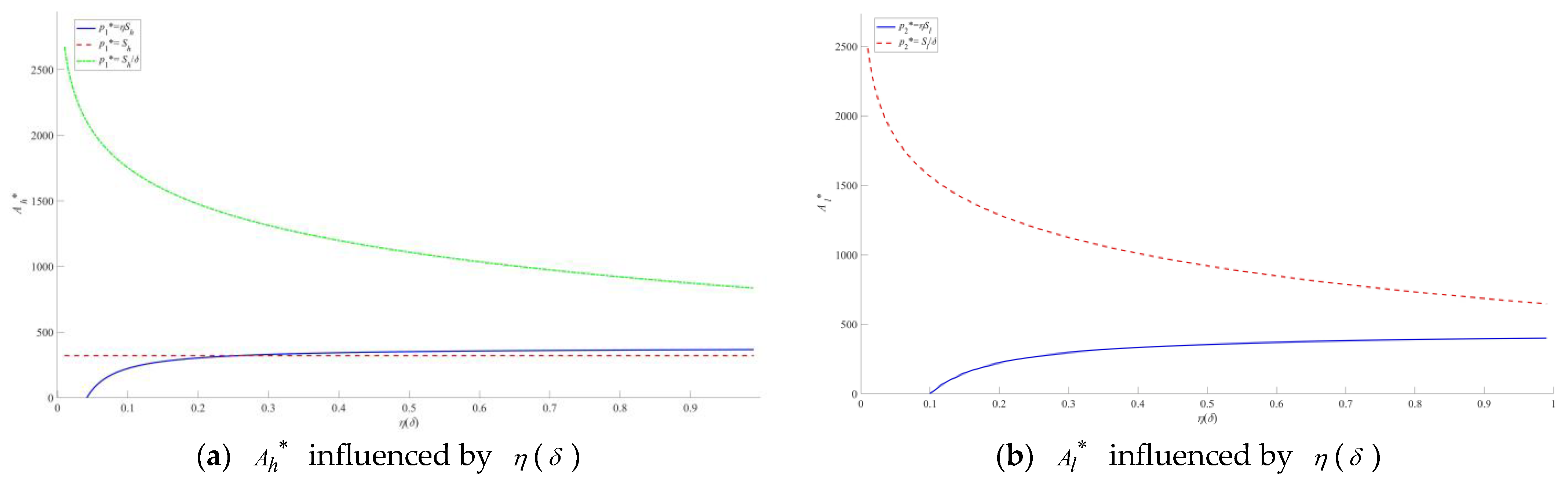
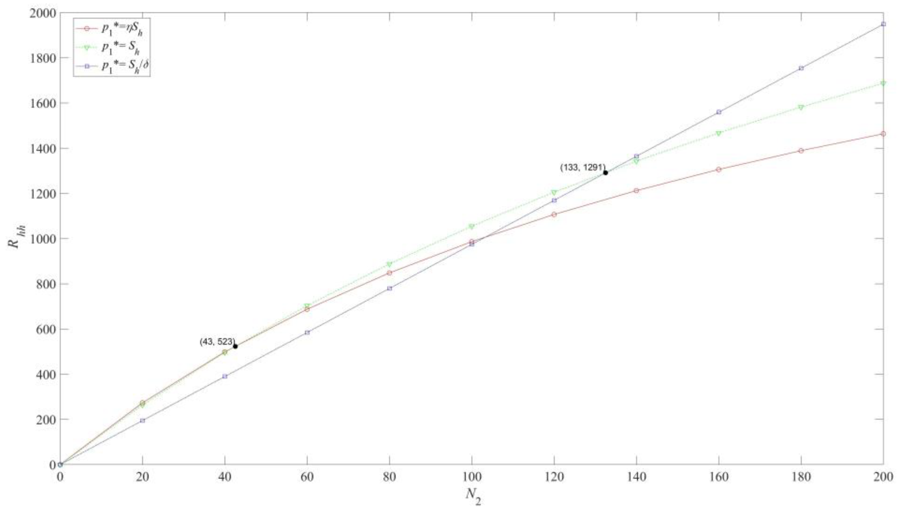
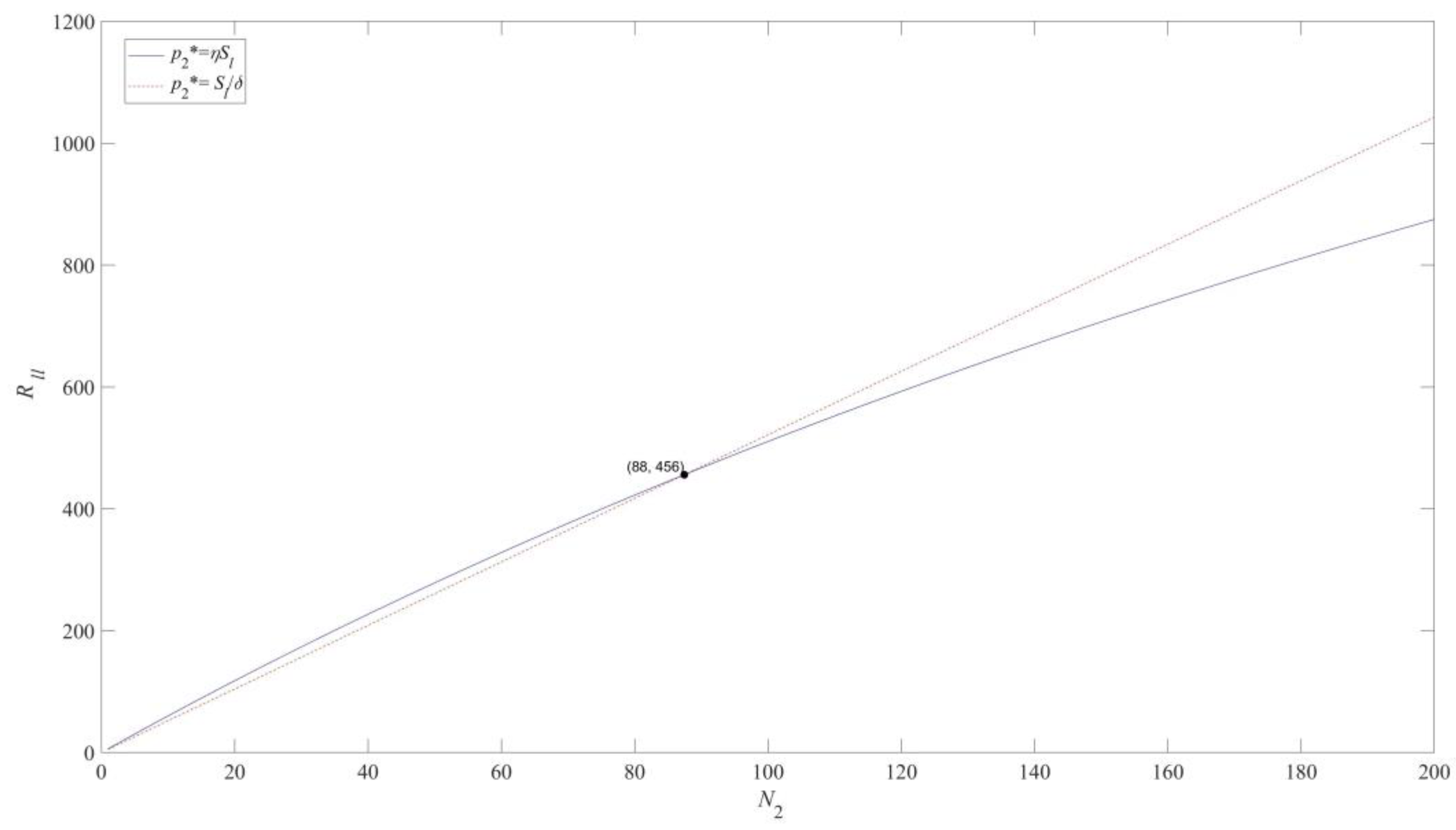
In the separating equilibrium, the optimal live-streaming strategies are
A h 2 * = η S h ( 3 ε A h 1 B 1 ) k η S h B 1 for   p 1 * = η S h S h ( 2 ε A h 1 B 2 ) k S h B 2 for   p 1 * = S h ( 1 β ) N 2 ln δ k S h ε A h 1 for   p 1 * = S h / δ
and
A l 2 * = η S l ( 2 ε A l 1 B 3 ) k η S l B 3 for   p 2 * = η S l ( 1 β ) N 2 ln δ k S l ε A l 1 for   p 2 * = S l / δ
(ii)
In the pooling equilibrium, the optimal live-streaming strategies are
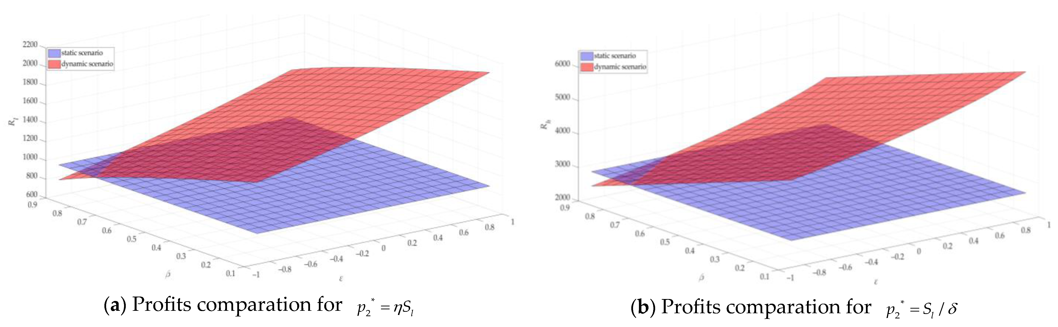
A m 2 * ( h ) = η ρ ( 3 ε A m 1 B 1 ) k η ρ B 1 for   p 1 * = η ρ S h ( 2 ε A m 1 B 2 ) k S h B 2 for   p 1 * = S h ( 1 β ) N 2 ln δ k ρ ε A m 1 for   p 1 * = ρ / δ
and
A m 2 * ( l ) = η ρ ( 2 ε A m 1 B 3 ) k η ρ B 3 for   p 2 * = η ρ ( 1 β ) N 2 ln δ k ρ ε A m 1 for   p 2 * = ρ / δ
where  B 1 = 1 N 1 + β ( N 2 + η N 3 ) + 1 ( 1 β ) N 2 + 1 ( 1 η β ) N 3 ,  B 2 = 1 N 1 + β ( N 2 + η N 3 ) + 1 ( 1 β ) N 2 , and  B 3 = 1 ( 1 β ) N 2 + 1 ( 1 η β ) N 3 .
See the Appendix A for proof.
Comparing the relationship between two strategies in dynamic scenario, Proposition 5 is derived.
Proposition 5.
There is a threshold,  ε ^ , for the impact coefficient,  ε , of the first-stage live-streaming strategy on the second stage. When ε < ε ^ , it holds that A q 2 * > A q 1 *   ( A m 2 * > A m 1 * ) . Otherwise, A q 2 * < A q 1 *   ( A m 2 * < A m 1 * )  holds.
See the Appendix A for proof.
Proposition 5 states that there is a threshold for the impact coefficient of the first-stage live-streaming strategy on the second stage. When the impact coefficient is less than this threshold, the enterprise is more inclined to make larger-scale live-streaming investments in the second stage. Otherwise, the enterprise needs to make sufficient investment in the first stage. The threshold is related to the number of potential consumers. The more potential consumers there are, the smaller the threshold. This finding highlights the dynamic nature of enterprise resource allocation [61]: in scenarios where the initial impact is weak, businesses tend to increase investments in the later stage to counteract diminishing marginal returns. Conversely, when the initial impact is strong, strategically concentrating resources to bolster existing advantages proves far more beneficial.
Next, we compare the profits between dynamic and static scenarios.
Proposition 6.
When the probability of high-quality project consumption by quality-sensitive consumers remains constant, a threshold ε ^  exists. If  ε > ε ^ , the profits in the dynamic scenario exceed those in the static scenario. Conversely, if ε < ε ^ , the profits in the static scenario surpass those in the dynamic scenario. Additionally, the profit differential between the dynamic and static scenarios consistently widens with the increase in ε .
See the Appendix A for proof.
Proposition 6 elaborates on the influence of the first-stage live-streaming strategy impact coefficient on the overall profit difference between dynamic and static scenarios when the probability of quality-sensitive consumers participating in high-quality projects remains constant. The research results indicate that when the impact coefficient exceeds the threshold, there will be a significant positive influence, leading to higher overall profits in the dynamic scenario than those in the static scenario. On the contrary, when the impact coefficient is smaller than the threshold, the profits in the static scenario exceed those in the dynamic scenario. In these two cases, the profit gap widens as the impact coefficient within the respective value range increases. These insights emphasize the pivotal role of the first-stage live-streaming strategy in driving profit results and highlight its strategic importance.
Proposition 7.
When the impact coefficient of the first-stage live-streaming strategy in the second stage remains constant:
(i)
There is a threshold  β ^ . The profits in the dynamic scenario are greater than in the static scenario when  β > β ^ , and the profits in the static scenario are greater than in the dynamic scenario when  β < β ^ .
(ii)
As β increases, when only quality-sensitive consumers participate in consumption, the profit gap continues to decrease. When multiple types of consumers participate, the profit gap first increases and then decreases.
See the Appendix A for proof.
Proposition 7 discusses the impact of the increased probability of high-quality project consumption by quality-sensitive consumers on the size relationship and difference of profits between dynamic and static scenarios when the impact coefficient of the first-stage live-streaming strategy on the second stage remains unchanged. Proposition 7 (i) finds that there is a threshold for the probability of increased consumption of high-quality projects by quality-sensitive consumers. When the probability exceeds the threshold, the profits in the dynamic scenario are greater than those in the static scenario. When the probability is less than the threshold, the profits in the static scenario are greater than those in the dynamic scenario. Proposition 7 (ii) finds that as the probability increases, when only quality-sensitive consumers participate in consumption, the profit gap decreases with increasing probability due to the negative impact of this probability increase on market demand in the dynamic scenario. The potential consumers in the second stage decrease, resulting in a continuous decrease in profits in the dynamic scenario. When there are multiple types of consumers, the profit gap increases first and then decreases with the increase in the probability due to changes in market demand.
Propositions 6 and 7 analyze the profit comparison between dynamic and static strategies, providing a reference for multi-stage or single-stage strategy selection for agricultural, cultural, and tourism enterprises [62]. Dynamic scenario profits can dramatically exceed static profits, provided that both the impact coefficient of the first-stage live-streaming strategy on the second stage and the likelihood of consumers gravitating towards the high-quality project surpass certain critical thresholds. This insight underscores the vital importance of two-stage live-streaming investments meeting dual conditions: early-stage strategies must evoke substantial positive impacts across stages, while consumers must cultivate a strong preference for the high-quality project. By meeting these conditions, enterprises can transcend static equilibrium and unlock the potential for global profit maximization through the strategic integration of resources over time.

6. Numerical Analysis

This section presents the numerical analysis for obtaining theoretical results in Section 4 and Section 5. The following parameter values are provided: a high-quality project usually results in high satisfaction, and consumers can obtain significant returns after purchasing. We assign a value of S h = 8 . Conversely, a low-quality project leads to low satisfaction, and the benefits obtained after purchasing will be smaller than those of high-quality projects, so let S l = 5 . According to the range of values of η and δ in Proposition 4, we set η = 0.5 and δ = 0.6 . Since there will be no negative live-streaming strategy, the value of k needs to meet A q * > 0 . Therefore, k = 1 is satisfied. To ensure a sufficiently large and differentiated consumer base, let N 1 = 300 , N 2 = 400 , N 3 = 500 .
Figure 2 depicts the dynamic evolution trajectory of the optimal live-streaming strategies for two types of projects when η and δ change in the separating equilibrium.
The optimal live-streaming strategy of the high-quality project is not affected by η or δ when p 1 * = S h . When p i * = η S q , the optimal live-streaming strategies consistently exhibit a monotonically increasing trend as η increases, and the growth trend gradually slows down. Conversely, for p i * = S q / δ , the optimal live-streaming strategies display a decreasing trend with the increase of δ, while the deceleration of this decreasing process tends to ease.
In the pooling equilibrium, the change curves of the optimal live-streaming strategies for the two projects closely resemble those in the separating equilibrium but are subject to the influence of consumers’ prior beliefs.
Figure 3 shows that as the quality of the project increases, the optimal live-streaming strategy for the enterprise becomes higher, but its growth rate slows down. As product quality improves, consumers are more willing to buy. Increasing live streaming investment can effectively attract potential consumers and boost sales.
In the pooling equilibrium, the analysis is similar.
Quality-sensitive consumers ( N 2 ) tend to make purchases in all situations, but their influence varies. Figure 4 and Figure 5 illustrate the impact of quality-conscious consumers on the strategic decisions of projects.
Figure 4 presents the profit curves for the high-quality project at different pricing levels, illustrating the impact of varying numbers of quality-sensitive consumers. When the count of quality-sensitive consumers is low, the high-quality project must employ lower pricing strategies to attract the other two consumer segments. However, as the number of quality-sensitive consumers grows, their contribution to overall profits increases significantly. When a special threshold is reached, which is the coordinate (45, 523) in the figure, the profits of low and medium prices are equal. After exceeding the threshold, the enterprise strategically shifts away from price-sensitive consumers and sets a higher price point of p 1 * = S h to optimize profitability. Furthermore, as the number of quality-sensitive consumers surpasses an even higher threshold, i.e., the coordinate (133, 1291) in the figure, they emerge as the primary driver of high-quality project profitability. The high-quality project attains maximum profit by implementing an exclusive premium pricing strategy of p 1 * = S h / δ and targeting this consumer segment.
Figure 5 illustrates the profound impact of the number of quality-sensitive consumers on the low-quality project’s income. When the number of quality-sensitive consumers is small, the enterprise needs to set a low price p 2 * = η S l to attract price-sensitive consumers. However, when the number of quality-sensitive consumers exceeds a certain threshold, i.e., the coordinate (88, 456) in the figure, they become the main source of income for the low-quality project. This shift in consumer behavior significantly impacts the low-quality project’s income, leading to the abandonment of price-sensitive consumers and setting a high price p 2 * = S l / δ to gain higher profit.
The comparisons of profits for the high- and low-quality projects concerning N 2 in the pooling equilibrium are similar to those in Figure 4 and Figure 5; thus, we will not go into detail here.
Figure 6 and Figure 7 compare the profit relationship between dynamic and static scenarios.
Figure 6a,b compare the profits of high-quality projects for the scenarios p 1 * = η S h and p 1 * = S h in the separating equilibrium. The dynamic scenario consistently yields higher profits than the static scenario. This is because there is a higher likelihood of quality-sensitive consumers choosing the high-quality project in the second stage, resulting in additional income. However, as this probability decreases, the growth rate of dynamic profits decreases. Figure 6c shows the profit comparisons for the high-quality project p 1 * = S h / δ in the separating equilibrium. In most cases, the dynamic scenario outperforms the static scenario. The only exception is when the first stage strategy significantly impacts the second stage negatively, and there is a substantial increase in the probability of quality-sensitive consumers choosing the high-quality project, thus causing consumer churn, which causes the static scenario to yield higher profits than the dynamic scenario.
In Figure 7, we observe a comparison of the profits of the low-quality project in the separating equilibrium. The absence of loyal consumers means that the profits of the low-quality project in the dynamic scenario may not always exceed those in the static scenario. Whether the pricing is high or low, the key factor is the increased probability of quality-sensitive consumers choosing the high-quality project in the second stage, along with the impact of the first-stage strategy on the second stage. This determines whether the profits in the static scenario exceed those in the dynamic scenario. However, if the increased probability does not significantly impact the outcome, the profits in the dynamic scenario will be higher.
The profits of the high- and low-quality projects concerning ε and β in the pooling equilibrium mirror those in Figure 6 and Figure 7, which will not go into detail here.

7. Conclusions

The primary distinction between our study and existing research is that previous studies have mainly concentrated on qualitative analyses and case studies of ACT. In contrast, we undertake quantitative research on ACT from a supply chain perspective. This approach allows for a more precise analysis of the profit structure within ACT enterprises and helps identify factors that might be overlooked in qualitative studies.
This article makes a certain exploratory contribution to enhancing the project promotion strategy of the ACT enterprise.
(1)
This study delivers a quantitative analysis of ACT projects from a supply chain perspective. By constructing utility functions for the ACT enterprise grounded in signaling game theory, we effectively compare their profitability across various scenarios.
(2)
We integrate consumer-type impacts into the profitability analysis of the ACT enterprise, categorizing consumers into three distinct groups based on previous research. This framework enhances the realism of optimal live-streaming strategies and provides actionable guidance for the successful implementation of ACT projects.

7.1. Research Results

This article explores how consumer types affect ACT enterprise’s pricing and live-streaming strategies in an information asymmetry environment and ultimately draws the following conclusions:
(i)
The existence of equilibrium mainly depends on the degree of punishment consumers impose for negative evaluations of the low-quality ACT project. When the degree of punishment exceeds a certain threshold, separating or pooling equilibrium will exist. Thus, only sufficiently severe punishment can curb opportunistic tendencies in the low-quality project. Considering the uncertainty of punishment intensity, there may be situations in the market where both separating and pooling equilibria are satisfied simultaneously. However, the LMSE criterion chooses the most profitable outcome for the high-quality project because it wants to reveal its type. Therefore, in this case, a pooling equilibrium exists.
(ii)
The types of consumers attracted by the ACT enterprise directly impact project pricing. When the enterprise targets only quality-sensitive consumers, the price is set at its highest. The price is moderate if it aims at both quality-oriented and quality-sensitive consumers. However, when the enterprise appeals to all types of consumers, the price becomes the lowest. It demonstrates that the pricing structure arises from the interplay between the varying preferences of consumers and the objective of maximizing profits for the enterprise. As the diversity of consumer types increases, the project price tends to decrease.
(iii)
The impact of the first-stage live-streaming strategy on the second stage has a specific threshold. When the effect is below this threshold, the influence of the first stage is relatively weak, indicating that the potential for using the first-stage live-streaming strategy to enhance the outcomes of the second stage is limited. In this case, the enterprise will likely invest more in the second stage to capture a larger market share. Conversely, when the impact exceeds this threshold, the enterprise should implement a more robust live-streaming strategy in the first stage. This strong positive effect can be a solid foundation for success in the subsequent stage.
(iv)
The profit advantage of the dynamic scenario is driven by two main factors: cross-stage strategic considerations and changes in consumer behavior. Consequently, in most instances, the profit from the dynamic scenario is higher than that from the static scenario. However, if quality-oriented consumers do not engage in consumption, the first-stage strategy can negatively impact the second stage. In this situation, the likelihood of consumers opting for the high-quality option significantly increases, resulting in profits from the static scenario exceeding those from the dynamic scenario.

7.2. Management Remark

Drawing upon the conclusions of the above research, we have distilled several managerial insights that can empower ACT companies to optimize their selection of live-streaming strategies, ultimately maximizing profits and promoting sustainable development.
(i)
Depending on the severity of penalties caused by negative consumer reviews, flexibly adopt either separating signals or pooling signals. Set low or high prices based on changes in the number of consumers and screen potential consumers.
(ii)
Monitoring the impact of the first-stage live-streaming strategy is crucial, as a positive influence that exceeds a certain threshold should prompt more investment in the first stage. In comparison, a negative impact should lead to more investment in the second stage.
(iii)
In situations where the live-streaming promotion environment in the second stage is unfavorable, opting for a live-streaming strategy tailored to the static scenario can help mitigate losses arising from negative impacts.

7.3. Limitations and Future Work

This study has made some strides in uncovering the optimal live-streaming strategies for the ACT enterprise. However, there are still some expandable aspects. While we have delved into two types of projects that a monopolistic enterprise might undertake, we can expand our analytical framework to consider oligopolistic markets. Additionally, the crucial interplay between the enterprise and live streaming platforms in terms of cooperation mode and benefit distribution deserves more attention. Lastly, the article overlooks the vital considerations of initial investment and the enterprise’s social responsibility, which are integral to a comprehensive strategic analysis.
In future work, we plan to conduct extensive research on the integrated development of ACT from the following perspectives: (1) Noncooperative games among multiple ACT enterprises. (2) The impact of the cooperation model between enterprises and live streaming platforms. (3) The investment of ACT enterprises in early-stage development and environmental protection.

Author Contributions

Conceptualization, F.M. and Y.W.; methodology, Y.W.; validation, F.M. and Y.W.; resources, F.M.; data curation, Y.W.; writing—original draft preparation, Y.W.; writing—review and editing, F.M. and Y.W.; funding acquisition, F.M. All authors have read and agreed to the published version of the manuscript.

Funding

This work was supported by the National Natural Science Foundation of China (No. 72371134), the National Social Science Fund of China (No. 22BJY019), the Ministry of Education Humanities and Social Science Foundation of China (No. 22YJ630061), and the Natural Science Foundation of Hunan Province of China (No. 2024JJ5451).

Institutional Review Board Statement

Not applicable.

Informed Consent Statement

Not applicable.

Data Availability Statement

Data are contained within the article.

Conflicts of Interest

The authors declare no conflicts of interest.

Abbreviations

The following abbreviation is used in this manuscript:
ACTAgriculture and cultural tourism

Appendix A

Proof of Lemma 1.
According to Equation (2), we derive R q p i = n T N n ( 1 e A q N n ) > 0 . Given that Rq is an increasing function for pi, and according to the domain definition of pi, it can be concluded that the optimal prices are p 1 * = η S h for   p 1 [ 0 , η S h ] S h for   p 1 ( η S h , S h ] S h / δ for   p 1 ( S h , S h / δ ] and p 2 * = η S l for   p 2 [ 0 , η S l ] S l / δ for   p 2 ( η S l , S l / δ ] . □
Proof of Lemma 2.
To streamline our calculations, we utilize Taylor’s formula to delve into the scenarios in Equations (5) and (6), ultimately yielding
R h h = η S h 2 ( 1 N 1 + 1 N 2 + 1 N 3 ) A h 2 + ( 3 η S h k ) A h for   p 1 * = η S h S h 2 ( 1 N 1 + 1 N 2 ) A h 2 + ( 2 S h k ) A h for   p 1 * = S h S h δ N 2 ( 1 e A h N 2 ) k A h for   p 1 * = S h / δ
and
R l l = S l 2 ( 1 N 2 + 1 N 3 ) A l 2 + ( 2 S l k ) A l for   p 2 * = η S l S l δ N 2 ( 1 e A l N 2 ) k A l for   p 2 * = S l / δ
Calculate the second-order partial derivatives of Equations (A1) and (A2) with respect to Ah and Al, respectively, and derive 2 R h h A h 2 = η S h ( 1 N 1 + 1 N 2 + 1 N 3 ) < 0 for   p 1 * = η S h S h ( 1 N 1 + 1 N 2 ) < 0 for   p 1 * = S h S h δ N 2 e A h N 2 < 0 for   p 1 * = S h / δ and 2 R l l A l 2 = S l ( 1 N 2 + 1 N 3 ) for   p 2 * = η S l S l δ N 2 e A l N 2 < 0 for   p 2 * = S l / δ .
Due to 2 R h h A h 2 < 0 and 2 R l l A l 2 < 0 , Equations (A1) and (A2) are strictly concave functions. Therefore, the optimal live-streaming strategies can be obtained from R h h A h = 0 and R l l A l = 0 , where A h * = 3 η S h k η S h ( 1 N 1 + 1 N 2 + 1 N 3 ) for   p 1 * = η S h 2 S h k S h ( 1 N 1 + 1 N 2 ) for   p 1 * = S h N 2 ln δ k S h for   p 1 * = S h / δ and A l * = 2 η S l k η S l ( 1 N 2 + 1 N 3 ) for   p 2 * = η S l N 2 ln δ k S l for   p 2 * = S l / δ . □
Proof of Proposition 1.
The quadratic Taylor expansion is applied to Equation (11), by which we have
R l h = η v 0 2 ( 1 N 2 + 1 N 3 ) A h 2 + ( 2 η v 0 k ) A h θ ( N 2 + N 3 ) f
Calculate the second-order partial derivatives of Equations (A3) and (11) for Ah, and derive 2 R l h A h 2 = η v 0 ( 1 N 2 + 1 N 3 ) for   Equation   A ( 3 ) v 0 δ N 2 e A h N 2 for   Equation   ( 11 ) ( 12 ) . Due to 2 R l h A h 2 < 0 , Equations (A3) and (11) are strictly concave functions. Hence, the optimal live-streaming strategies are obtained as follows: A h * = 2 η v 0 k η v 0 ( 1 N 2 + 1 N 3 ) for   p 2 * = η v 0 N 2 ln δ k v 0 for   p 2 * = v 0 / δ by setting R l h A h = 0 . Additionally, the maximum profits of sending a high-quality signal for a low-quality project are derived as R l h * = ( 2 η v 0 k ) 2 2 η v 0 ( 1 N 2 + 1 N 3 ) θ ( N 2 + N 3 ) f for   p 2 * = η v 0 v 0 N 2 δ k N 2 + k N 2 ln δ k v 0 θ N 2 f for   p 2 * = v 0 / δ . Under the condition of Equation (12), the requirement for the establishment of the separating equilibrium is f ( 4 η 2 S l v 0 k 2 ) ( v 0 S l ) a S l v 0 ( N 2 + N 3 ) for   p 2 * = η S l f v 0 S l + δ k ln S l v 0 δ θ for   p 2 * = S l / δ where a = 2 θ η ( 1 N 2 + 1 N 3 ) . □
Proof of Proposition 2.
Similar to the proof of Proposition 1, the requirements for the establishment of a pooling equilibrium are 9 η 2 S h ρ k 2 1 for   p 1 * = η ρ δ k ln S h ρ 1 for   p 1 * = S h and f ( 4 η 2 ρ v 0 k 2 ) ( v 0 ρ ) a ρ v 0 ( N 2 + N 3 ) for   p 2 * = η ρ f v 0 δ k + k ln δ k v 0 θ ( 2 η ρ k ) 2 a ρ N 2 for   p 2 * = ρ / δ . □
Proof of Proposition 3 (i).
When f 1 > f 3 , according to Equations (13) and (24), we have 4 η 2 ρ S l k 2 > 0 , by which R l m * > R l l * . Whether it is f > f 1 > f 3 or f 1 > f > f 3 , there is always R h m * R h h * . Therefore, only the pooling equilibrium exists. Conversely, we obtain R l m * < R l l * when f 1 < f 3 . In this case, when f 3 > f f 1 , we drive R h m * < R h h * ; when f f 3 > f 1 , we obtain R h m * R h h * . The former indicates that only a separating equilibrium exists, while the latter suggests that the low-quality project prefers the separating equilibrium and the high-quality project is more inclined toward the pooling equilibrium. Since the LMSE refinement aims to identify the most lucrative outcome for the high-quality project, it endeavors to disclose its type. Consequently, in the latter scenario, the pooling equilibrium exists. □
The proof of (ii) is identical to that of (i) and is therefore omitted.
Proof of Proposition 4.
(i)
According to Equations (5), (7) and (9), the maximum profits of the high-quality project in the separating equilibrium can be derived as
R h h * = ( 3 η S h k ) 2 2 η S h ( 1 N 1 + 1 N 2 + 1 N 3 ) for   p 1 * = η S h ( 2 S h k ) 2 2 S h ( 1 N 1 + 1 N 2 ) for   p 1 * = S h S h N 2 δ k N 2 + k N 2 ln δ k S h for   p 1 * = S h / δ
Let (A4) be represented as R h h 1 * , R h h 2 * , and R h h 3 * , respectively.
(i-1) assuming maximum profit is achieved when p 1 * = η S h . From R h h 1 * > R h h 2 * , we obtain N 1 N 2 N 3 ( N 1 + N 2 ) < ( 3 η S h k ) 2 η ( 2 S h k ) 2 1 . The inequality only makes sense when ( 3 η S h k ) 2 η ( 2 S h k ) 2 1 > 0 , that is, ( 3 η S h k ) 2 η ( 2 S h k ) 2 > 0 . Define Π 1 = ( 3 η S h k ) 2 η ( 2 S h k ) 2 . Since Π 1 is a quadratic function about η whose Δ = ( 4 S h 2 + 8 S h k + k 2 ) ( 2 S h k ) 2 > 0 , there exists η, such that Π 1 > 0 , where η ( 0 , H H 2 36 S h 2 k 2 18 S h 2 ) ( H + H 2 36 S h 2 k 2 18 S h 2 , 1 ) . From R h h 1 * > R h h 3 * , we derive N 2 ( 1 N 1 + 1 N 3 ) < ( 3 η S h k ) 2 2 η S h ( S h δ k + k ln δ k S h ) 1 . The inequality only makes sense when ( 3 η S h k ) 2 2 η S h ( S h δ k + k ln δ k S h ) 1 > 0 , that is, ( 3 η S h k ) 2 2 η S h ( S h δ k + k ln δ k S h ) > 0 . Define Π 2 = ( 3 η S h k ) 2 2 η S h ( S h δ k + k ln δ k S h ) . From N 2 ln δ k S h > 0 , we derive S h > δ k and Π 2 δ = 2 η S h ( S h δ k ) δ 2 > 0 . Therefore, Π 2 is monotonically increasing in relation to δ . Let Π 2 = 0 , we obtain δ 0 = S h LambertW ( e 9 η 2 S h 2 4 η S h k + k 2 2 η S h k ) k . When δ 0 < 1 , there exists δ ( δ 0 , 1 ) such that Π 2 > 0 .
Similar to (i-1), one can derive the conclusions for (i-2) and (i-3).
(i)
From Equations (6), (8) and (10), the maximum profits of the low-quality project in the separating equilibrium are derived as follows:
R l l * = ( 2 η S l k ) 2 2 η S l ( 1 N 2 + 1 N 3 ) for   p 2 * = η S l S l N 2 δ k N 2 + k N 2 ln δ k S l for   p 2 * = S l / δ
Let (A5) be represented as R l l 1 * and R l l 2 * .
(ii-1) assuming maximum profit is achieved when p 2 * = η S l . From R l l 1 * > R l l 2 * , we have δ ( δ 0 , 1 ) when δ 0 = S l LambertW ( e 4 η S l 2 2 η S l k + k 2 2 η S l k ) k <1. The proof of (ii-2) is similar to that of (ii-1) and is therefore omitted. □
Proof of Lemma 5.
The quadratic Taylor expansion is applied to Equation (26), by which we have
R h s e p = 1 2 η S h B 1 A h 2 2 + [ η S h ( 3 ε B 1 A h 1 ) k ] A h 2 + C 1 for   p 1 * = η S h 1 2 S h B 2 A h 2 2 + [ S h ( 2 ε B 2 A h 1 ) k ] A h 2 + C 2 for   p 1 * = S h ( S h δ ) ( 1 β ) N 2 Y h 1 k A h 2 + R h 1 s e p for   p 1 * = S h / δ
where B 1 = 1 N 1 + β ( N 2 + η N 3 ) + 1 ( 1 β ) N 2 + 1 ( 1 η β ) N 3 , C 1 = η S h ( ε 2 A h 1 2 2 B 1 + 3 ε A h 1 ) + R h 1 s e p , B 2 = 1 N 1 + β ( N 2 + η N 3 ) + 1 ( 1 β ) N 2 , and C 2 = S h ( ε 2 A h 1 2 2 B 2 + 2 ε A h 1 ) + R h 1 s e p .
Calculate the second-order partial derivative of Equation (A6) with respect to Ah and derive 2 R h s e p A h 2 2 = η S h B 1 for   p 1 * = η S h S h B 2 for   p 1 * = S h S h δ ( 1 β ) N 2 e A h 2 + ε A h 1 ( 1 β ) N 2 for   p 1 * = S h / δ . Due to 2 R h s e p A h 2 2 < 0 , Equation (A6) is strictly concave function. Therefore, we derive A h 2 * = η S h ( 3 ε B 1 A h 1 ) k η S h B 1 for   p 1 * = η S h S h ( 2 ε B 2 A h 1 ) k S h B 2 for   p 1 * = S h ( 1 β ) N 2 ln δ k S h ε A h 1 for   p 1 * = S h / δ under the condition of R h s e p A h 2 = 0 .
The expressions of A l 2 * and A m 2 * can be obtained in a similar way to A h 2 * . □
Proof of Proposition 5.
When the optimal live-streaming strategy for the second stage is larger than that of the first stage, we obtain
k B ε 2 + 3 η S h B ε + M < 0
where M = ( 3 η S h k ) [ B 1 ( 1 N 1 + 1 N 2 + 1 N 3 ) ] . Solving Equation (A7), it yields 3 η S h B 1 ( 3 η S h B 1 ) 2 4 k B 1 M 2 k B 1 < ε < 3 η S h B 1 + ( 3 η S h B 1 ) 2 4 k B 1 M 2 k B 1 . According to Equation (9), we obtain 3 η S h > k . Thus, 3 η S h B 1 + ( 3 η S h B 1 ) 2 4 k B 1 M 2 k B 1 < 1 . Furthermore, considering the function Π 3 = k B ε 2 + 3 η S h B ε + M whose symmetry axis is 3 η S h 2 k such that 3 η S h 2 k < 1 2 , it implies that 3 η S h B 1 ( 3 η S h B 1 ) 2 4 k B 1 M 2 k B 1 < 1 . Therefore, A q 2 * > A q 1 * when 1 < ε < 3 η S h B 1 + ( 3 η S h B 1 ) 2 4 k B 1 M 2 k B 1 . Otherwise, A q 2 * < A q 1 * . □
The conclusions for situations can be proven in the same way.
Proof of Proposition 6.
Let Ω r (r = 1, 2, 3, 4) be expressed as the difference between the profit of the enterprise in the dynamic and static scenario. In the separating equilibrium, according to Equations (5), (6), (36) and (37), we have
Ω 1 = η S h ( 3 ε A h 1 ε 2 A h 1 2 B 1 2 ) + [ η S h ( 3 ε A h 1 B 1 k ) ] 2 2 η S h B 1 ε 2 k 2 2 η S h ( 1 N 1 + 1 N 2 + 1 N 3 ) for   p 1 * = η S h S h ( 2 ε A h 1 ε 2 A h 1 2 B 2 2 ) + [ S h ( 2 ε A h 1 B 2 k ) ] 2 2 S h B 2 ε 2 k 2 2 S h ( 1 N 1 + 1 N 2 ) for   p 1 * = S h β N 2 ( S h δ k + k ln δ k S h ) k ε N 2 ln δ k ( 1 ε ) S h + N 2 [ S h δ k ( 1 ε ) + k ln δ k ( 1 ε ) S h ] for   p 1 * = S h / δ
for the high-quality project, and
Ω 2 = η S l ( 2 ε A l 1 ε 2 A l 1 2 B 3 2 ) + [ η S l ( 2 ε A l 1 B 3 k ) ] 2 2 η S l B 3 ε 2 k 2 2 η S l ( 1 N 2 + 1 N 3 ) for   p 2 * = η S l β N 2 ( S l δ k + k ln δ k S l ) k ε N 2 ln δ k ( 1 ε ) S l + N 2 [ S l δ k ( 1 ε ) + k ln δ k ( 1 ε ) S l ] for   p 2 * = S l / δ
for the low-quality project.
In the pooling equilibrium, according to Equations (16), (17), (44) and (45), we obtain
Ω 3 = η ρ ( 3 ε A h 1 ε 2 A h 1 2 B 1 2 ) + [ η ρ ( 3 ε A h 1 B 1 k ) ] 2 2 η ρ B 1 ε 2 k 2 2 η ρ ( 1 N 1 + 1 N 2 + 1 N 3 ) for   p 1 * = η S h S h ( 2 ε A h 1 ε 2 A h 1 2 B 2 2 ) + [ S h ( 2 ε A h 1 B 2 k ) ] 2 2 S h B 2 ε 2 k 2 2 S h ( 1 N 1 + 1 N 2 ) for   p 1 * = S h β N 2 ( ρ δ k + k ln δ k ρ ) k ε N 2 ln δ k ( 1 ε ) ρ + N 2 [ ρ δ k ( 1 ε ) + k ln δ k ( 1 ε ) ρ ] for   p 1 * = S h / δ
for the high-quality project, and
Ω 4 = η S l ( 2 ε A l 1 ε 2 A l 1 2 B 3 2 ) + [ η S l ( 2 ε A l 1 B 3 k ) ] 2 2 η S l B 3 ε 2 k 2 2 η S l ( 1 N 2 + 1 N 3 ) for   p 2 * = η S l β N 2 ( S l δ k + k ln δ k S l ) k ε N 2 ln δ k ( 1 ε ) S l + N 2 [ S l δ k ( 1 ε ) + k ln δ k ( 1 ε ) S l ] for   p 2 * = S l / δ
for the low-quality project.
According to (A8) and (A9), we obtain Ω 1 ε = [ ( ε 1 ) k 2 + 3 η S h k ] N 1 N 2 N 3 η S h [ N 1 ( N 2 + N 3 ) + N 2 N 3 ] for   p 1 * = η S h N 1 N 2 k ( 2 S h k + ε k ) S h ( N 1 + N 2 ) for   p 1 * = S h k N 2 ln δ k ( 1 ε ) S h for   p 1 * = S h / δ for the high-quality project, and Ω 2 ε = N 2 N 3 k ( 2 η S l k + ε k ) S l ( N 2 + N 3 ) for   p 2 * = η S l k N 2 ln δ k ( 1 ε ) S l for   p 2 * = S l / δ for the low-quality project.
From Equations (A10) and (A11), we obtain Ω 3 ε = [ ( ε 1 ) k 2 + 3 η ρ k ] N 1 N 2 N 3 η ρ [ N 1 ( N 2 + N 3 ) + N 2 N 3 ] for   p 1 * = η S h N 1 N 2 k ( 2 S h k + ε k ) S h ( N 1 + N 2 ) for   p 1 * = S h k N 2 ln δ k ( 1 ε ) ρ for   p 1 * = S h / δ for the high-quality project, and Ω 4 ε = N 2 N 3 k ( 2 η ρ k + ε k ) ρ ( N 2 + N 3 ) for   p 2 * = η S l k N 2 ln δ k ( 1 ε ) ρ for   p 2 * = S l / δ for the low-quality project.
The disparity in profits between dynamic and static increases with the growth of ε. This means that as the impact intensifies, the profit gap between dynamic and static widens. It is important to note that there exists a threshold ε   ^ , such that Ω r = 0 . In the dynamic scenario, profits outstrip those in the static scenario if ε > ε   ^ . Conversely, if ε < ε   ^ , the static scenario yields greater profits than the dynamic scenario. □
Proof of Proposition 7.
i
Let Ω r (r = 1, 2, 3, 4) be shown as the difference between the profit of the enterprise in the dynamic and static scenario. There exists a threshold β ^ for each r such that Ω r = 0 . In a dynamic scenario, profits exceed those in the static scenario when β < β ^ . Conversely, in the static scenario, profits surpass those in the dynamic scenario when β > β ^ .
ii
According to Lemma 5, we need to calculate the first- and second-order partial derivatives of Bn (n = 1, 2, 3) with respect to β, where
B 1 β = N 2 + η N 3 [ N 1 + β ( N 2 + η N 3 ) ] 2 + 1 ( 1 β ) 2 N 2 + 1 ( 1 η β ) 2 N 3 2 B 1 β 2 = 2 ( N 2 + η N 3 ) 2 [ N 1 + β ( N 2 + η N 3 ) ] 3 + 2 ( 1 β ) 3 N 2 + 2 η 2 ( 1 η β ) 3 N 3
B 1 β = N 2 + η N 3 [ N 1 + β ( N 2 + η N 3 ) ] 2 + 1 ( 1 β ) 2 N 2 2 B 2 β 2 = 2 ( N 2 + η N 3 ) 2 [ N 1 + β ( N 2 + η N 3 ) ] 3 + 2 ( 1 β ) 3 N 2
B 3 β = N 2 + η N 3 [ N 1 + β ( N 2 + η N 3 ) ] 2 + 1 ( 1 η β ) 2 N 3 2 B 3 β 2 = 2 ( N 2 + η N 3 ) 2 [ N 1 + β ( N 2 + η N 3 ) ] 3 + 2 η 2 ( 1 η β ) 3 N 3
It is easy to observe that 2 B n β 2 > 0 . Thus, B n β increases monotonically with respect to β. There is B n β > 0 when β 1 , and there is a possibility that B n β < 0 when β 0 . Therefore, there is a threshold β ^ n , when 0 β β ^ n , Bn decreases monotonically with respect to β; when β ^ n < β < 1  Bn increases monotonically in relation to β.
In the separating equilibrium:
For p 1 * = η S h , according to Equation (A8), we derive Ω 1 B 1 = ( 3 η S h k ) 2 2 η S h B 1 2 < 0 . In addition, inspired by Equation (A12), Ω 1 increases steadily with respect to β when 0 β β ^ 1 , and Ω 1 decreases steadily with respect to β when β ^ 1 < β < 1 .
For p 1 * = S h , from Equation (A8), we have Ω 1 B 2 = 2 ( S h k 2 ) 2 S h B 2 2 < 0 . Additionally, inspired by Equation (A13), Ω 1 increases monotonically with respect to β when 0 β β ^ 2 , and Ω 1 decreases monotonically with respect to β when β ^ 2 < β < 1 .
For p 1 * = S h / δ , according to Equation (A8), we obtain Ω 1 β = N 2 ( S h δ k + k ln δ k S h ) δ < 0 which indicates that Ω 1 decreases monotonically with respect to β.
For p 2 * = η S l , from Equation (A9), we obtain Ω 2 B 3 = 2 ( η S l k 2 ) 2 η S l B 3 2 < 0 . In addition, according to Equation (A14), Ω 2 increases monotonically with respect to β when 0 β β ^ 3 , and Ω 2 decreases monotonically with respect to β when β ^ 3 < β < 1 .
For p 2 * = S l / δ , according to Equation (A9), we acquire Ω 2 β = N 2 ( S l δ k + k ln δ k S l ) δ < 0 . Thus, Ω 2 decreases monotonically with respect to β. □
Similar to the separating equilibrium, one can check that all conclusions for the pooling equilibrium hold.

References

  1. Chodkowska-Miszczuk, J.; Szymańska, D. Agricultural biogas plants—A chance for diversification of agriculture in Poland. Renew. Sustain. Energy Rev. 2013, 20, 514–518. [Google Scholar] [CrossRef]
  2. Addai, G.; Suh, J.; Bardsley, D.; Robinson, G.; Guodaar, L. Exploring sustainable development within rural regions in Ghana: A rural web approach. Sustain. Dev. 2024, 32, 3890–3907. [Google Scholar] [CrossRef]
  3. Ammirato, S.; Felicetti, A.M.; Raso, C.; Pansera, B.A.; Violi, A. Agritourism and Sustainability: What We Can Learn from a Systematic Literature Review. Sustainability 2020, 12, 9575. [Google Scholar] [CrossRef]
  4. Luo, Y.; Xiong, T.; Meng, D.; Gao, A.; Chen, Y. Does the Integrated Development of Agriculture and Tourism Promote Farmers’ Income Growth? Evidence from Southwestern China. Agriculture 2023, 13, 1817. [Google Scholar] [CrossRef]
  5. Wang, J.; Zhou, F.; Xie, A.; Shi, J. Impacts of the integral development of agriculture and tourism on agricultural eco-efficiency: A case study of two river basins in China. Environ. Dev. Sustain. 2024, 26, 1701–1730. [Google Scholar] [CrossRef]
  6. Ohe, Y. Impact of Rural Tourism Operated by Retiree Farmers on Multifunctionality: Evidence from Chiba, Japan. Asia Pac. J. Tour. Res. 2008, 13, 343–356. [Google Scholar] [CrossRef]
  7. Jiang, G. How Does Agro-Tourism Integration Influence the Rebound Effect of China’s Agricultural Eco-Efficiency? An Economic Development Perspective. Front. Environ. Sci. 2022, 10, 921103. [Google Scholar] [CrossRef]
  8. Xie, C.; Yu, J.; Huang, S.S.; Zhang, J. Tourism e-commerce live streaming: Identifying and testing a value-based marketing framework from the live streamer perspective. Tour. Manag. 2022, 91, 104479. [Google Scholar] [CrossRef]
  9. Ye, C.; Zheng, R.; Li, L. The effect of visual and interactive features of tourism live streaming on tourism consumers’ willingness to participate. Asia Pac. J. Tour. Res. 2022, 27, 506–525. [Google Scholar] [CrossRef]
  10. McKinney, L.N. Creating a satisfying internet shopping experience via atmospheric variables. Int. J. Consum. Stud. 2004, 28, 268–283. [Google Scholar] [CrossRef]
  11. Barbieri, C. Agritourism research: A perspective article. Tour. Rev. 2020, 75, 149–152. [Google Scholar] [CrossRef]
  12. Ilbery, B.W. Farm diversification as an adjustment strategy on the urban fringe of the West Midlands. J. Rural Stud. 1991, 7, 207–218. [Google Scholar] [CrossRef]
  13. Sonnino, R. For a ‘Piece of Bread’? Interpreting Sustainable Development through Agritourism in Southern Tuscany. Sociol. Rural. 2004, 44, 15. [Google Scholar] [CrossRef]
  14. Pearce, P.L. Farm tourism in New Zealand: A social situation analysis. Ann. Tour. Res. 1990, 17, 337–352. [Google Scholar] [CrossRef]
  15. Fleischer, A.; Tchetchik, A. Does rural tourism benefit from agriculture? Tour. Manag. 2005, 26, 493–501. [Google Scholar] [CrossRef]
  16. Mohammad, N.; Masood, K. Farm tourism as a driving force for socioeconomic development: A benefits viewpoint from Iran. Curr. Issues Tour. 2021, 24, 247–263. [Google Scholar]
  17. Gong, J.-Z.; Jian, Y.-Q.; Chen, W.-L.; Liu, Y.-S.; Hu, Y.-M. Transitions in rural settlements and implications for rural revitalization in Guangdong Province. J. Rural. Stud. 2022, 93, 359–366. [Google Scholar] [CrossRef]
  18. Tang, C.-C.; Liu, Y.; Wan, Z.-W.; Liang, W.-Q. Evaluation system and influencing paths for the integration of culture and tourism in traditional villages. J. Geogr. Sci. 2023, 33, 2489–2510. [Google Scholar] [CrossRef]
  19. Wu, J.; Wan, T. Innovative Practice of Heavy Metal Soil Remediation Technology under the Background of Rural Revitalization by Integrating Agriculture, Culture and Tourism. Pol. J. Environ. Stud. 2024, 33, 4407–4419. [Google Scholar] [CrossRef]
  20. Sun, Y.; Shao, X.; Li, X.-T.; Guo, Y.; Nie, K. A 2020 perspective on “How live streaming influences purchase intentions in social commerce: An IT affordance perspective”. Electron. Commer. Res. Appl. 2020, 40, 100958. [Google Scholar] [CrossRef]
  21. Liu, P.; Zhang, R.; Wang, Y.; Yang, H.-L.; Liu, B. Manufacturer’s sales format selection and information sharing strategy of platform with a private brand. J. Bus. Ind. Mark. 2024, 39, 244–255. [Google Scholar] [CrossRef]
  22. Xu, P.; Cui, B.-J.; Lyu, B. Influence of Streamer’s Social Capital on Purchase Intention in Live Streaming E-Commerce. Front. Psychol. 2022, 12, 748172. [Google Scholar] [CrossRef]
  23. Ang, T.; Wei, S.-Q.; Anaza, N.A. Livestreaming vs pre-recorded. Eur. J. Mark. 2018, 52, 2075–2104. [Google Scholar] [CrossRef]
  24. Ma, L.; Gao, S.; Zhang, X. How to Use Live Streaming to Improve Consumer Purchase Intentions: Evidence from China. Sustainability 2022, 14, 1045. [Google Scholar] [CrossRef]
  25. Wu, G.-K.; Yang, W.-S.; Hou, X.-R.; Tian, Y.-D. Agri-food supply chain under live streaming and government subsidies: Strategy selection of subsidy recipients and sales agreements. Comput. Ind. Eng. 2023, 185, 107563. [Google Scholar] [CrossRef]
  26. Xin, B.-G.; Hao, Y.-R.; Xie, L. Strategic product showcasing mode of E-commerce live streaming. J. Retail. Consum. Serv. 2023, 73, 103360. [Google Scholar] [CrossRef]
  27. Gao, J.-Y.; Zhao, X.-J.; Zhai, M.-F.; Zhang, D.; Li, G. AI or Human? The Effect of Streamer Types on Consumer Purchase Intention in Live Streaming. Int. J. Hum. –Comput. Interact. 2024, 41, 305–317. [Google Scholar] [CrossRef]
  28. Ji, M.; Chen, X.-Y.; Wei, S.-B. What Motivates Consumers’ Purchase Intentions in E-Commerce Live Streaming: A Socio-Technical Perspective. Int. J. Hum. –Comput. Interact. 2024, 41, 1585–1605. [Google Scholar] [CrossRef]
  29. Lv, J.; Cao, C.; Xu, Q.-W.; Ni, L.-Y.; Shao, X.-Y.; Shi, Y.-Y. How Live Streaming Interactions and Their Visual Stimuli Affect Users’ Sustained Engagement Behaviour—A Comparative Experiment Using Live and Virtual Live Streaming. Sustainability 2022, 14, 8907. [Google Scholar] [CrossRef]
  30. Xu, Y.-J.; Zeng, K.; Guo, J.; Li, X.; Dong, L.-C.; Jiang, W.-Q. Whether Live Streaming Has a Better Performance? An Examination of Product Presentation Modes on Cross-Border E-Commerce Platform. Int. J. Hum.–Comput. Interact. 2023, 41, 69–84. [Google Scholar] [CrossRef]
  31. Guo, J.; Xu, Y.-J.; Jiang, W.-Q.; Li, Y. The Influences of Live Streaming Affordance in Cross-Border E-Commerce Platforms: An Information Transparency Perspective. J. Glob. Inf. Manag. (JGIM) 2021, 30, 1–24. [Google Scholar]
  32. Chen, A.-H.; Zhang, Y.-N.; Liu, Y.-T.; Lu, Y.-B. Be a good speaker in livestream shopping: A speech act theory perspective. Electron. Commer. Res. Appl. 2023, 61, 101190. [Google Scholar] [CrossRef]
  33. Guo, Y.-Y.; Zhang, K.-X.; Wang, C.-Y. Way to success: Understanding top streamer’s popularity and influence from the perspective of source characteristics. J. Retail. Consum. Serv. 2022, 64, 102788. [Google Scholar] [CrossRef]
  34. Luo, H.-Y.; Cheng, S.-J.; Zhou, W.-H.; Yu, S.-M.; Lin, X.-D. A Study on the Impact of Linguistic Persuasive Styles on the Sales Volume of Live Streaming Products in Social E-Commerce Environment. Mathematics 2021, 9, 1576. [Google Scholar] [CrossRef]
  35. Ma, X.-Y.; Liu, S. Information disclosure strategies of live-streaming supply chains in the digi-economy era. Manag. Decis. Econ. 2024, 45, 17. [Google Scholar] [CrossRef]
  36. Boyacı, T.; Akçay, Y. Pricing When Customers Have Limited Attention. Manag. Sci. 2017, 64, 2995–3014. [Google Scholar] [CrossRef]
  37. Chen, L.-D.; Xu, Q.-Y.; He, Y. Channel selection strategy with consumer impulse purchase in livestream selling. Manag. Decis. Econ. 2024, 45, 5006–5019. [Google Scholar] [CrossRef]
  38. Prince, C.A.; Fang, J.; Ohemeng, A.A.; Bakabbey, K.N. Customer engagement and purchase intention in live-streaming digital marketing platforms. Serv. Ind. J. 2021, 41, 767–786. [Google Scholar]
  39. Park, J.; Kim, R.B. A new approach to segmenting multichannel shoppers in Korea and the U.S. J. Retail. Consum. Serv. 2018, 45, 163–178. [Google Scholar] [CrossRef]
  40. Huseynov, F.; Yıldırım, S.Ö. Online Consumer Typologies and Their Shopping Behaviors in B2C E-Commerce Platforms. SAGE Open 2019, 9, 2158244019854639. [Google Scholar] [CrossRef]
  41. Zhan, Z.-F.; Huang, Y.-H. A study on omnichannel retailers’ return strategies considering showroom and consumer preference behavior. Manag. Decis. Econ. 2024, 45, 4763–4776. [Google Scholar] [CrossRef]
  42. Zhen, X.-P.; Cai, G.-S.; Song, R.; Jang, S. The effects of herding and word of mouth in a two-period advertising signaling model. Eur. J. Oper. Res. 2019, 275, 361–373. [Google Scholar] [CrossRef]
  43. Zhao, J.; Qiu, J.; Zhou, Y.-W.; Hu, X.-J.; Yang, A.-F. Quality disclosure in the presence of strategic consumers. J. Retail. Consum. Serv. 2020, 55, 102084. [Google Scholar] [CrossRef]
  44. Liu, Z.; Chen, H.-R.; Zhang, X.-M.; Gajpal, Y.; Zhang, Z.-C. Optimal channel strategy for an e-seller: Whether and when to introduce live streaming? Electron. Commer. Res. Appl. 2024, 63, 101348. [Google Scholar] [CrossRef]
  45. Guo, X.-W.; Zha, Y.; Chen, H.-P.; Liang, L. National brand manufacturers’ supply strategy in the presence of retailers’ store-branded lookalike packaging and consumer confusion about quality preference. Transp. Res. Part E 2023, 175, 102679. [Google Scholar] [CrossRef]
  46. Han, X.-Y.; Liu, X. Equilibrium decisions for multi-firms considering consumer quality preference. Int. J. Prod. Econ. 2020, 227, 107688. [Google Scholar] [CrossRef]
  47. Örsdemir, A.; Kemahlıoğlu-Ziya, E.; Parlaktürk, A.K. Competitive Quality Choice and Remanufacturing. Prod. Oper. Manag. 2014, 23, 48–64. [Google Scholar] [CrossRef]
  48. Bagwell, K. Chapter 28 The Economic Analysis of Advertising. Handb. Ind. Organ. 2007, 3, 143. [Google Scholar]
  49. Spence, M. Job Market Signaling*. Q. J. Econ. 1973, 87, 355–374. [Google Scholar] [CrossRef]
  50. Ahn, Y.; Lee, J. The Impact of Online Reviews on Consumers’ Purchase Intentions: Examining the Social Influence of Online Reviews, Group Similarity, and Self-Construal. J. Theor. Appl. Electron. Commer. Res. 2024, 19, 1060–1078. [Google Scholar] [CrossRef]
  51. Xu, X.-X.; Fan, R.-G.; Wang, D.-X.; Wang, Y.-T.; Wang, Y.-Y. The role of consumer reviews in e-commerce platform credit supervision: A signaling game model based on complex network. Electron. Commer. Res. Appl. 2024, 63, 101347. [Google Scholar] [CrossRef]
  52. Zhang, X.-B.; Tu, Y.-B.; Haney, M.H.; Cheng, H.-W. Buyers’ Negative Ratings and Textual Comments on eBay: Reasons for Posting Ratings and Factors in Denouncing Sellers. J. Theor. Appl. Electron. Commer. Res. 2024, 19, 1717–1733. [Google Scholar] [CrossRef]
  53. Jiang, B.-J.; Tian, L.; Xu, Y.-F.; Zhang, F.-Q. To Share or Not to Share: Demand Forecast Sharing in a Distribution Channel. Mark. Sci. 2016, 35, 800–809. [Google Scholar] [CrossRef]
  54. Li, Q.-Y.; Ding, H.; Shi, T.-Q.; Tang, Y.-L. To share or not to share: The optimal advertising effort with asymmetric advertising effectiveness. Ann. Oper. Res. 2020, 329, 1–28. [Google Scholar] [CrossRef]
  55. Tian, L.; Jiang, B.-J. Comment on “Strategic Information Management Under Leakage in a Supply Chain”. Manag. Sci. 2016, 63, 4258–4260. [Google Scholar] [CrossRef]
  56. Mayzlin, D.; Dover, Y.; Chevalie, J. Promotional Reviews: An Empirical Investigation of Online Review Manipulation. Am. Econ. Rev. 2014, 104, 2421–2455. [Google Scholar] [CrossRef]
  57. Krishnamoorthy, A.; Prasad, A.; Sethi, S. Optimal pricing and advertising in a durable-good duopoly. Eur. J. Oper. Res. 2010, 200, 486–497. [Google Scholar] [CrossRef]
  58. Luo, L.; Li, X.; Zhao, Y. A two-stage stochastic-robust model for supply chain network design problem under disruptions and endogenous demand uncertainty. Transp. Res. Part E 2025, 196, 104013. [Google Scholar] [CrossRef]
  59. Chen, Y.-F. Herd behavior in purchasing books online. Comput. Hum. Behav. 2008, 24, 1977–1992. [Google Scholar] [CrossRef]
  60. Mai, E.-P.; Liao, Y. The interplay of word-of-mouth and customer value on B2B sales performance in a digital platform: An expectancy value theory perspective. J. Bus. Ind. Mark. 2022, 37, 1389–1401. [Google Scholar] [CrossRef]
  61. Ujwary-Gil, A.; Potoczek, N.R. A dynamic, network and resource-based approach to the sustainable business model. Electron. Mark. 2020, 30, 717–733. [Google Scholar] [CrossRef]
  62. Ljungqvist, A.; Wilhelm, W.J. IPO Pricing in the Dot-Com Bubble. J. Financ. 2003, 58, 723–752. [Google Scholar] [CrossRef]
Figure 1. Game sequence.
Jtaer 20 00089 g001
Figure 2. Optimal live-streaming strategy curves for η and δ in the separating equilibrium.
Jtaer 20 00089 g002
Figure 3. Optimal live-streaming strategy curves for S q in the separating equilibrium.
Jtaer 20 00089 g003
Figure 4. Profit comparison of the high-quality project in the separating equilibrium.
Jtaer 20 00089 g004
Figure 5. Profit comparison of the low-quality project in the separating equilibrium.
Jtaer 20 00089 g005
Figure 6. The profits of the high-quality project in the separating equilibrium.
Jtaer 20 00089 g006
Figure 7. The profits of the low-quality project in the separating equilibrium.
Jtaer 20 00089 g007
Table 1. Summary of parameters and decision variables.
SymbolDescription
Parameters
q The project type, q = h , l
k The cost per unit of live streaming
S q The benefit of consumers
η The discount coefficient of quality concerns for price-sensitive consumers, 0 < η < 1
δ The discount coefficient of price concerns for quality-sensitive consumers, 0 < δ < v / S h
v The consumers’ perception of the quality of the project before consumption
N 1 The number of quality-oriented consumers
N 2 The number of quality-sensitive consumers
N 3 The number of price-sensitive consumers
α / 1 α The probability of the project being of high or low quality
f The punishment for the enterprise due to negative consumer reviews
d q The market demand
λ / 1 λ The probability of adopting a high/low live-streaming strategy for the low-quality project
θ The proportion of consumers who give negative reviews to the low-quality project
β The increased probability of quality-sensitive consumers purchasing the high-quality project, 0 β < 1
ε The impact of the first-stage live-streaming strategy on the second stage, 1 < ε < 1
Decision variables
A q / A m The live-streaming strategy in the static separating/pooling equilibrium
A q t / A m t The live-streaming strategy of the tth stage ( t = 1 , 2 ) in the dynamic separating/pooling equilibrium
p i The price of the high- ( i = 1 )/low-quality ( i = 2 ) project
Disclaimer/Publisher’s Note: The statements, opinions and data contained in all publications are solely those of the individual author(s) and contributor(s) and not of MDPI and/or the editor(s). MDPI and/or the editor(s) disclaim responsibility for any injury to people or property resulting from any ideas, methods, instructions or products referred to in the content.

