Customer-Centric Decision-Making with XAI and Counterfactual Explanations for Churn Mitigation

Abstract

In this paper, we propose a methodology designed to deliver actionable insights that help businesses retain customers. While Machine Learning (ML) techniques predict whether a customer is likely to churn, this alone is not enough. Explainable Artificial Intelligence (XAI) methods, such as SHapley Additive Explanations (SHAP) and Local Interpretable Model-agnostic Explanations (LIME), highlight the features influencing the prediction, but businesses need strategies to prevent churn. Counterfactual (CF) explanations bridge this gap by identifying the minimal changes in the business–customer relationship that could shift an outcome from churn to retention, offering steps to enhance customer loyalty and reduce losses to competitors. These explanations might not fully align with business constraints; however, alternative scenarios can be developed to achieve the same objective. Among the six classifiers used to detect churn cases, the Balanced Random Forest classifier was selected for its superior performance, achieving the highest recall score of 0.72. After classification, Diverse Counterfactual Explanations with ML (DiCEML) through Mixed-Integer Linear Programming (MILP) is applied to obtain the required changes in the features, as well as in the range permitted by the business itself. We further apply DiCEML to uncover potential biases within the model, calculating the disparate impact of some features.

1. Introduction

1.1. General Context

The integration of eXplainable Artificial Intelligence (XAI) into customer churn prediction has become a pressing need in business environments. It represents an issue for organizations across industries, from telecommunications and banking to e-commerce and software as a service. As businesses adopt machine learning (ML) to identify at-risk customers, a challenge lies in understanding the rationale behind model predictions [1,2]. One promising solution is the application of counterfactual (CF) explanations, particularly through the Diverse Counterfactual Explanations (DiCE) method and its adaptation for ML, known as DiCEML.

CF explanations present an alternative to traditional interpretability methods. Instead of approximating a ML model or ranking features based on their predictive significance, CF explanations actively probe the model to identify the fewest changes needed to alter its decision [3,4]. DiCEML, in particular, generates such explanations by providing feature-modified variations in an input that would have led to a different outcome. In essence, CF explanations guide individuals on the actionable steps they can take to achieve a desired outcome rather than highlighting influential features.

In the context of churn prediction, the goal is not only to identify which customers are likely to leave but to uncover what specific changes in behavior or conditions might alter that outcome. This shifts the focus from passive prediction to proactive intervention. DiCEML fits within this framework by providing CF scenarios that suggest minimal and diverse changes to customer features, which, if implemented, could shift the prediction from “churn” to “no churn”. These explanations go beyond traditional feature importance by enabling individualized, actionable insights.

1.2. Challenges and Motivation for This Research

However, there are several challenges associated with applying DiCEML in churn-related tasks [5,6,7]. One major issue is the complexity and imbalance of churn datasets, where non-churners outnumber churners, leading to biased models and unreliable CF explanations [8]. Additionally, while many explanation methods identify influential features, they often fall short in addressing whether the suggested changes are realistic or feasible in practice [9]. There is also an ongoing debate regarding the reliability and ethical implications of CF explanations. Some scholars argue that CF explanations reflect correlations rather than true causal relationships, which could mislead users into making ineffective or unethical decisions. Others worry that CF reasoning, if not properly constrained, could lead to discriminatory practices, such as offering retention incentives only to certain customer demographics [10,11]. Despite these concerns, the motivation for researching DiCEML in the domain of churn prediction is obvious. Businesses seek not only to predict churn but to prevent it, and this requires actionable, trustworthy insights. DiCEML provides a method to generate such insights in a way that is both data-driven and interpretable. It offers the potential to personalize retention strategies, enhance customer relationships and allocate retention resources more efficiently.

1.3. Objectives and Research Questions

In this context, our paper introduces a methodology designed to go beyond prediction and deliver actionable and constraint-aware interventions to support customer retention. The methodology combines ML-based classification with DiCEML. After training six classifiers to detect potential churners, we select the best classifier model for its superior recall performance, an important metric when the goal is to minimize false negatives in identifying customers at risk. Once potential churners are identified, DiCEML is applied to generate diverse and realistic CF scenarios that comply with business-imposed constraints on feature changes. Moreover, DiCEML also serves a second, equally important function: it helps uncover potential biases within the ML models. By analyzing which features frequently appear in CF explanations, businesses may audit the model’s decision logic and ensure that it does not reinforce discriminatory or unjust patterns, such as systematically assigning a higher churn risk to certain demographic groups.

The objectives of our research include:

(a)

developing a hybrid churn prediction and intervention system that integrates classification with constraint-aware CF reasoning;

(b)

evaluating the quality, diversity and feasibility of CF generated by DiCEML;

(c)

and investigating the method’s utility in detecting and mitigating model biases.

These objectives position the research at the intersection of XAI, business intelligence and ethical AI. Thus, several research questions (RQ) are formulated: RQ1: How can DiCEML be used to generate realistic and diverse CF explanations for churn predictions under business constraints? RQ2: To what extent can these explanations support targeted and effective customer retention strategies in real-world settings? RQ3: How do the explanations generated by DiCEML compare to those from other XAI techniques in terms of interpretability, feasibility and actionability? RQ4: Can DiCEML effectively expose and mitigate the biases embedded in churn prediction models?

2. Literature Review

One work surveyed recent methods for generating CF explanations in interpretable ML [1]. CF explanations help clarify what changes in an input would lead to a different prediction, such as what a bank customer would need to change to get a loan approved, for instance. The authors categorized existing explainers by their methodological approach and labeled them according to the characteristics and properties of the generated CF explanation. They also conducted visual and quantitative benchmarking, evaluating criteria like minimality, actionability, stability, diversity, discriminative power and runtime. The findings showed that no current method satisfies all desired properties simultaneously, highlighting the need for further advancements in CF explanation techniques. Furthermore, other studies addressed the growing need for interpretability in churn prediction models [12,13,14,15]. One of them focused on CF explanations, which provided intuitive, instance-level insights by showing how small changes in input could alter a model’s prediction [16]. It highlighted a gap: existing CF learning approaches often overlook the effects of class imbalance and the location of instances within customer data. To tackle this, the authors proposed a novel approach that explicitly incorporated these factors. Their experimental results showed that both class imbalance and instance location significantly influenced the success rate, proximity, sparsity and credibility of CF explanations. Moreover, Ref. [17] examined consumer behavior in online entertainment shopping, a novel e-commerce model typically driven by pay-to-bid auction mechanisms. The authors developed a dynamic structural model that captured how consumers learn from both personal participation and observational learning based on historical auction data. Using a large dataset from a real entertainment shopping website, the research found that consumers initially joined due to a significant overestimation of the entertainment value and an underestimation of auction competition. Over time, as learning occurred, participation rates declined. The model explained the consumer churn phenomenon, identifying two distinct consumer types: risk-averse users, who left the platform early, and risk-seeking users, who remained engaged and overcommitted to the auctions. Through CF simulations, the researchers evaluated how different policy changes could influence user behavior.

Another research paper explored how to build trust in AI systems like ChatGPT through plausible CF explanations [9]. The authors proposed a multi-objective framework that balances plausibility, change intensity and adversarial power using a GAN-based model and a custom solver. Tested on six classification tasks with image and 3D data, the framework revealed a trade-off among objectives, produced explanations aligned with human reasoning and exposed biases and misrepresented attributes in model inputs. Other authors addressed the challenge of efficiently generating CF explanations for prototype-based classifiers, such as Learning Vector Quantization (LVQ) models, which are important in the context of explainability and legal requirements like the EU’s GDPR [7]. They developed convex and non-convex optimization programs, tailored to the metric used, to compute traditional input-based CF explanations. They also introduced a novel perspective by proposing model-based CF: instead of altering the input, they explored minimal changes to the model itself (specifically, its metric parameters) required to change the prediction.

A fast, model-agnostic method was proposed by [18] for generating interpretable CF explanations using class prototypes. By leveraging either encoders or class-specific k-d trees, the method significantly reduced search time and improved the interpretability of CF explanations. The approach was evaluated on both image and tabular datasets showing strong performance. The method avoided the computational overhead of numerical gradient evaluation. Another research introduced collective CF explanations as a novel approach to post hoc interpretability in ML, particularly for high-stakes decision-making [19]. Unlike traditional methods that generate a single CF per instance, this method provided CF explanations for a group of instances, aiming to minimize the total perturbation cost under shared constraints. Using mathematical optimization models, the authors identified features critical across the dataset for shifting predictions to a desired class. Their approach also allowed hybrid treatment, where some instances could still receive individual CF explanations, helping to detect and handle outliers. Under specific assumptions, the problem was reduced to a convex quadratic mixed-integer optimization task, solvable to optimality on moderate-sized datasets. Results on real-world data demonstrated the method’s effectiveness and practicality for stakeholder-centric explanations.

Another research paper addressed the challenge of improving the interpretability of ML predictions by proposing a novel method for generating CF explanations [20]. While existing methods like DiCE, Proto and RF-OCSE can generate CF explanations, they either fail to clearly identify causal features or are limited to specific model types (e.g., tree ensembles). To overcome these limitations, the authors introduced a CF Explanation Generation method with Minimal Feature Boundary (CEGMFB). The approach was tested against six baseline methods across 16 datasets and a real-world case study, showing that CEGMFB consistently outperformed existing methods, offering more efficient and targeted CF explanations. Achievable Minimally-Contrastive Counterfactuals (AMCC) was further introduced [21], a novel model-agnostic method designed to generate real-time, feasible CF explanations for complex black-box models. Unlike traditional explanation methods, AMCC focused on actionable interventions, making it suitable for dynamic settings like question answering or decision support systems. The method first created high-precision instance-based explanations, then narrowed the CF search space using domain-specific constraints to find practical, minimal changes. Evaluated on a well-known dataset with a 90% accurate classifier, AMCC successfully produced CF explanations in 47% of cases, with an average generation time of just 80 milliseconds.

Multi-Layer Perceptron (MLP) for fault detection in photovoltaic (PV) arrays and its interpretability were further tested [22]. To enhance transparency and trust, the authors applied three explainable AI (XAI) techniques: SHAP, Anchors and DiCE, each representing different types of local explanations. Using an MLP model with 99.11% accuracy, the results showed that SHAP provided the explanations most aligned with domain knowledge, offering clear insights into model behavior. Moreover, the authors of [23] developed an interpretable early warning system for Multiple Organ Dysfunction Syndrome (MODS) using ML, aiming to enable early prediction, risk factor identification and automated intervention suggestions. The authors employed several ML models and improved prediction accuracy using a stacked ensemble method (SuperLearner). For interpretability, they used Kernel-SHAP to identify risk factors and DiCE to generate actionable CF interventions. Trained and tested on the MIMIC-III and MIMIC-IV datasets, the SuperLearner achieved the best overall performance, with a Yordon index of 0.813, sensitivity of 0.884, accuracy of 0.893 and utility score of 0.763. The DWNN model had the highest AUC (0.960) and specificity (0.935). Predictors included the GCS score, MODS scores related to GCS and creatinine, with strong odds ratios indicating their influence.

Another study explored the use of CF explanations to enhance the explainability and trust of AI models in predicting student success [24]. While traditional methods like feature importance offer general insights, they fall short in addressing the individual-level causal effects crucial for personalized support. The authors applied multiple ML models to predict course outcomes (pass/fail). They then used DiCE to analyze how changes in specific behaviors could shift predictions from failing to passing. The findings revealed that altering certain social media usage scenarios could positively impact student outcomes. A user study with educators further validated the usefulness of CF, showing that educators found them valuable for understanding and supporting student performance through tailored interventions. Furthermore, the authors of [25] proposed SAC-FACT, a novel approach that leverages reinforcement learning (RL), specifically the Soft Actor-Critic (SAC) architecture, for generating CF explanations in a model-agnostic, scalable and optimal way. Unlike traditional optimization or heuristic-based CF methods, SAC-FACT addresses the complex constraints and large search space inherent to CF explanation generation using RL. The method is designed to generate CF explanations that satisfy properties such as validity, diversity, proximity and sparsity, by carefully modeling the reward function. Experiments on four real-world datasets demonstrated that SAC-FACT converges effectively and outperforms existing methods like DiCE and SingleCF in generating CF explanations.

Comparing the previous research (as in

Table 1. A comparison of previous research.

Ref.	Objective	Methods	Main Results
[1]	Survey CF explanation techniques in interpretable ML	Benchmarking CF methods across metrics like minimality, actionability, stability, etc.	No existing method satisfied all desirable CF properties; need for further improvement identified
[16]	Improve CF explanations in churn prediction, considering class imbalance and data distribution	Novel CF generation incorporating class imbalance and instance location	Class imbalance and instance location impact CF quality; success rate and credibility vary across methods
[17]	Understand user churn in entertainment e-commerce platforms	Dynamic structural model and CF simulations	Identified risk-averse and risk-seeking users; policy-based CFs revealed insights into user retention strategies
[9]	Build trust in AI through plausible CF explanations	Multi-objective GAN-based CF generation framework	Balanced plausibility, change intensity, and adversarial robustness; identified model bias and misrepresented inputs
[7]	Generate CFs for prototype-based classifiers and meet GDPR requirements	Convex and non-convex optimization + model-based CFs (parameter changes)	Introduced model-level CFs; ensured explainability and compliance with legal standards
[18]	Develop a fast, interpretable CF method	Model-agnostic method using encoders or k-d trees, with class prototypes	Reduced runtime and improved CF interpretability; addressed categorical features efficiently
[19]	Propose collective CF explanations for groups	Mixed-integer quadratic optimization with shared constraints	Efficient group-level CFs; hybrid individual-group treatment helped handle outliers; stakeholder-aligned explanations
[20]	Overcome limitations of existing CF methods by better targeting causal features	CEGMFB—CF Explanation Generation with Minimal Feature Boundary	Outperformed 6 baseline methods on 16 datasets; delivered precise, feature-focused CFs
[21]	Generate fast, real-time CF explanations for dynamic systems	AMCC—instance-based explanations with domain constraints	Feasible CFs in 47% of cases within 80 ms; enabled actionable insights in real-time applications
[22]	Interpret MLP-based PV fault detection model using XAI	SHAP, Anchors, and DiCE for interpretability	SHAP offered domain-aligned explanations; DiCE provided actionable CFs for fault understanding
[23]	Create an interpretable early warning system for MODS	SuperLearner ensemble + Kernel-SHAP + DiCE	Best performance across metrics; actionable interventions improved clinical decision-making
[24]	Enhance student performance prediction and support via CF explanations	ML models + DiCE for individual-level behavioral intervention	DiCE-based CFs improved educational outcomes; educators validated their practical usefulness
[25]	Develop a scalable RL-based CF generation approach	SAC-FACT—Reinforcement Learning with Soft Actor-Critic	Achieved high-quality CFs with key properties; outperformed DiCE and SingleCF in 4 datasets

) with our proposal, the latter introduces a comprehensive and practical methodology for customer churn management. While previous studies have focused on churn prediction or model explainability, our approach is distinctive in its integration of ML with actionable business strategies, using CF explanations as a bridge.

An essential novelty in our work is the integration of predictive modeling with real-world intervention strategies. While ML methods predict whether a customer is likely to churn and explainability tools like SHAP or LIME indicate which features drive that prediction, our research recognizes that these alone do not suffice for decision-making in business contexts. Our methodology addresses this gap by moving beyond static interpretation and introducing CF reasoning to identify the minimal, feasible changes that would shift a customer’s outcome from churn to retention. We also use the same framework to detect potential biases in the model, allowing the methodology to serve both as a tool for customer retention and auditing.

3. Materials and Methods

3.1. Input Data

The input dataset (IBM Telco Churn dataset) we use in the simulation (7043 rows and 21 columns) (Telco customer churn (11.1.3+)) consists of four categories of columns/variables, as shown in

Table 2. Categories, features and their descriptions.

Category	Feature	Description
Customer information variables	customerID	Unique identifier for each customer
	Gender	The customer’s gender (Male/Female)
	SeniorCitizen	Whether the customer is a senior citizen (0 = No, 1 = Yes)
	Partner	Whether the customer has a partner (Yes/No)
	Dependents	Whether the customer has dependents (Yes/No)
Service subscription variables	Tenure	Number of months the customer has been with the company
	PhoneService	Whether the customer has a phone service (Yes/No)
	MultipleLines	Whether the customer has multiple lines (No, Yes, No phone service)
	InternetService	Type of internet service (DSL, Fiber optic, No)
	OnlineSecurity	Whether the customer has online security service (Yes, No, No internet service)
	OnlineBackup	Whether the customer has an online backup service (Yes, No, No internet service)
	DeviceProtection	Whether the customer has device protection (Yes, No, No internet service)
	TechSupport	Whether the customer has tech support service (Yes, No, No internet service)
	StreamingTV	Whether the customer has a TV streaming service (Yes, No, No internet service)
	StreamingMovies	Whether the customer has a movie streaming service (Yes, No, No internet service)
Contract and billing information	Contract	Type of contract the customer has (Month-to-month, One year, Two year)
	PaperlessBilling	Whether the customer has opted for paperless billing (Yes/No)
	PaymentMethod	Method of payment (Electronic check, Mailed check, Bank transfer (automatic), Credit card (automatic))
	MonthlyCharges	Monthly charge amount the customer pays
	TotalCharges	Total amount charged to the customer during their tenure
Target variable	Churn	Whether the customer has churned (Yes/No)

. The first category includes demographic data, the second category includes service subscription data, the third category includes contract and bulling data, whereas the fourth category notes whether the customer churned or not. The total number of non-null values in

Table 3. Features, non-null count and their type.

Column	Non-Null Count	Type
customerID	7043	object
Gender	7043	object
SeniorCitizen	7043	int64
Partner	7043	object
Dependents	7043	object
Tenure	7043	int64
PhoneService	7043	object
MultipleLines	7043	object
InternetService	7043	object
OnlineSecurity	7043	object
OnlineBackup	7043	object
DeviceProtection	7043	object
TechSupport	7043	object
StreamingTV	7043	object
StreamingMovies	7043	object
Contract	7043	object
PaperlessBilling	7043	object
PaymentMethod	7043	object
MonthlyCharges	7043	float64
TotalCharges	7043	object
Churn	7043	object

indicates that the dataset is complete and contains no missing values. The data types include object, int64 and float64, which reflect whether the feature is categorical, integer or continuous numeric, respectively. For categorical features, we applied the One-Hot Encoding technique using the get_dummies method in Python (version 3.12).

Significantly more customers did not churn, as indicated by the green bar labeled “No”, which represents over 5000 customers. In contrast, the pink bar labeled “Yes” shows that fewer than 2000 customers churned (as in Figure 1), suggesting an imbalance in the dataset.

Figure 2a shows that customers who churned are more concentrated in the early months of tenure, especially around the 1 to 6-month range. Thus, churn is more likely to happen early in a customer’s lifecycle. On the other hand, customers with a longer tenure (especially those near the 70-month mark) are far more likely to stay, as seen by the green bar at the end. Figure 2b shows how customers are distributed based on their monthly charges and total charges, while also distinguishing between those who churned and those who did not. Customers with lower total charges (generally on the left side of the plot) include a relatively high number of churn cases. This suggests that customers who churn often leave early, before they accumulate high total charges, even if they are paying relatively high monthly rates. Meanwhile, customers with high total charges (toward the right) are mostly non-churned, indicating that they have been with the company longer and are more likely to remain. There is a dense concentration of churned customers with monthly charges above USD 70 and total charges below USD 2000, reinforcing the idea that high monthly charges early in the customer lifecycle increases the likelihood of churn.

Figure 3a compares the number of customers who churned and did not churn across three different contract types: Month-to-month, One year and Two year. It shows that churn is most common among customers with month-to-month contracts. While this group has the highest overall number of customers, it also shows a relatively large portion of churners compared to the other two contract types. In contrast, customers with one-year and two-year contracts have much lower churn rates. The two-year contract group has the fewest churned customers, suggesting that longer contracts are associated with greater customer retention. Figure 3b shows how churn varies depending on the customer’s method of payment. Customers using electronic checks have the highest churn rate, as the pink bar for this method is almost as long as the green bar. This suggests that electronic check users are more likely to leave the service. In contrast, automatic payments, whether by bank transfer or credit card, are associated with significantly lower churn, as shown by the relatively small pink segments and dominant green bars. Mailed checks also show a relatively low churn rate.

3.2. Methodology

The mathematical model of churn classification and CF explanations using DiCE ML starts with the problem definition that is churn classification. Let $X\subseteq {\mathbb{R}}^n$ be the feature space, where each instance $x_i$ represents a customer with a set of attributes:

$$x_i=(x_{i1},x_{i2},\dots ,x_{in})$$

(1)

where $x_i$ can be either continuous (e.g., MonthlyCharges, TotalCharges, tenure) or categorical (e.g., Contract, PaymentMethod, InternetService). Y is the binary target variable:

$$Y=\left\{\mathrm{0,1}\right\},0=NonChurn,1=Churn$$

(2)

The goal is to learn a function f: X → [0, 1] that outputs the probability $P$ of churn:

$$P\left(Y=1∣X\right)=f\left(X;\theta \right)$$

(3)

where $\theta$ represents model parameters (e.g., weights in logistic regression or a neural network [26]).

Then, the classifier makes predictions:

$$\widehat{y}=\left\{\begin{array}{c}1,iff\left(x\right)\ge \tau \\ 0,iff\left(x\right)<\tau \end{array}\right.$$

(4)

where $\tau$ is a predefined threshold, often set to 0.5.

CF explanation implies finding minimal feature changes. For a customer predicted to churn (f(X) = 1), our goal is to find a minimal perturbation ΔX such that the model prediction switches from churn (1) to non-churn (0). With this goal, we define a CF instance X′ such that the following is true:

X′ = X + ΔX

(5)

where ΔX is a small, actionable modification satisfying the following:

f(X′) = 0

(6)

To formulate the optimization problem, we solve the following:

$${\underset{∆X}{\min }‖∆X‖}_p$$

(7)

subject to:

f(X + ΔX) = 0

(8)

where ${‖∆X‖}_p$ represents a norm measuring the magnitude of changes. Common choices: ${‖∆X‖}_1$ (L1 norm) encourages sparse modifications (changing as few features as possible); ${‖∆X‖}_2$ (L2 norm) penalizes large deviations.

Actionability constraints means certain features (e.g., gender) should not be modified, categorical values should remain valid (e.g., switching from “Month-to-Month” to “Two Year” is allowed, but not an arbitrary numeric value), and monetary features (e.g., MonthlyCharges) should be within a reasonable/permitted range.

Thus, the final optimization problem is as follows:

$${\underset{∆X}{\min }‖∆X‖}_1$$

(9)

subject to:

f(X + ΔX) = 0, ΔX ∈ A

(10)

where A represents the set of actionable feature changes.

DiCEML is designed to generate CF examples for ML models [24,27], where feature construction and processing are essential [28]. By MILP, DiCEML identifies the minimal modifications needed in input instances to alter the model’s prediction to a desired outcome. Thus, DiCEML generates CF explanations by simulating small, realistic changes to features. Based on business logic and historical patterns, the following features are expected to be most influential:

(a)

Contract Type $x_{contract}$ Changing from “Month-to-Month” to “One Year” or “Two Year” may reduce the risk of churn.

∆𝑥_{𝑐𝑜𝑛𝑡𝑟𝑎𝑐𝑡} = “One Year” → “MonthtoMonth”

(11)

(b)

Tech Support and Online Security $x_{techsupport}$, $x_{onlinesecurity}$. Enabling these services may lower churn.

∆𝑥_techsupport = 1; ∆𝑥_{𝑜𝑛𝑙𝑖𝑛𝑒𝑠𝑒𝑐𝑢𝑟𝑖𝑡𝑦} = 1

(12)

(c)

Monthly Charges $x_{monthly}$. Lowering monthly fees (within reason) can retain customers.

$$∆x_{monthly}<0$$

(13)

(d)

Tenure $x_{tenure}$. Increasing tenure (simulating loyalty discounts) may reduce churn.

$$∆x_{tenure}>0$$

(14)

Thus, the minimal CF explanation for converting a churned customer (f(X) = 1) to a retained customer (f(X) = 0) may involve a small subset of these feature changes.

3.3. Classifiers

In order to classify the customers, we train six models: Balanced Random Forest (BRF) [29], Random Forest (RF), eXtreme Gradient Boost (XGB), Light Gradient Boost Machine (LGBM), Logistic Regression and Decision Tree (DT). Other models such as recurrent neural networks, genetic algorithms and Support Vector Machine could be used [30,31,32] to predict churn. As in most cases of classification, the target is unbalanced. The BRF extends the RF by addressing the target imbalance. The minority classes are represented during training, reducing bias towards the majority class. Each decision tree in the forest is trained on a balanced subset of data. Instead of drawing random samples from the full dataset, BRF performs balanced bootstrapping, where each sample is drawn with equal representation of each class. Unlike standard RF, which may favor majority classes, BRF ensures fair decision-making across all classes. For each tree, BRF selects a subset of data by undersampling the majority class to match the size of the minority class. Each tree is trained on a different balanced subset of the dataset. At the prediction time, each tree gives a vote and the final classification is determined by majority voting.

A standard RF classifier constructs decision trees, where each tree is trained on a bootstrap sample of the original dataset. Each decision tree learns a mapping:

$$f_t:X\to Y$$

(15)

where t is the tree index.

For prediction, RF aggregates predictions from all trees:

$$\widehat{y}=mode{\left\{f_t\left(x\right)\right\}}_{t=1}^T$$

(16)

The difference in BRF is that each bootstrap sample is balanced. Instead of drawing a random sample, BRF ensures that each class contributes equally. For each tree t, select $n_{min}$ samples from each class $C_i$, where

$$n_{min}=min\left(\left|C_1\right|,\left|C_2\right|,\dots ,\left|C_k\right|\right)$$

(17)

This ensures an equal number of samples per class. Each decision tree splits data based on an impurity criterion:

$$Gini=1-\sum _{i=1}^k{p}_i^2$$

(18)

$$H\left(X\right)=-\sum _{i=1}^k{p}_i{log}_2\left(p_i\right)$$

(19)

where $p_i$ is the probability of class i at a given node.

The final classification is determined by aggregating votes from all decision trees. RF has an option to weight classes (class_weights), and synthetic data generation techniques such as SMOTE [33] and ADASYN can be added to balance the target. A brief comparison is provided in

Table 4. A comparison: BRF, RF and SMOTE/ADASYN+RF.

Method	Sampling Strategy	Bias Towards Majority Class	Performance on Imbalanced Data
Standard RF	Random sampling	High	Poor
BRF	Class-balanced bootstrapping	Low	Better generalization
SMOTE/ADASYN+RF	Synthetic data generation	Moderate	Can introduce noise

.

The BRF classifier addresses class imbalance more effectively, and how it compares to other popular classifiers like RF, XGB, LGBM, LR and DT is shown in

Table 5. Comparison of classifiers.

Model	Handling Imbalance	Bias Toward Majority	Computational Complexity	Interpretability	Performance on Imbalanced Data	Suitability for Large Datasets
BRF	Yes (Balanced Bootstrapping)	Low	Medium-High	Moderate	High	Moderate
RF	No (Needs Resampling)	High	High	Moderate	Poor	High
XGB	Yes (Weighted Loss, SMOTE, Scale_Pos_Weight)	Medium	High	Low	High	Very High
LGBM	Yes (Boosting + Weighted Loss)	Medium	Medium-High	Low	High	Very High
LR	No (Needs Class Weights)	High	Low	High	Poor	Moderate
DT	No (Needs Class Weights)	High	Low	High	Poor	Moderate

.

Compared to RF, BRF performs better in imbalanced classification tasks without requiring external sampling techniques. XGB and LGBM outperform BRF for large-scale data but require hyperparameter tuning. LR and DT are simpler models but usually fail on highly imbalanced datasets.

When evaluating the performance of a classification ML model, various metrics can be used depending on the specific problem type [34,35]. Accuracy is a good metric in general for balanced datasets, but misleading for imbalanced datasets.

$$Accuracy={\displaystyle \frac{TP+TN}{TP+TN+FP+FN}}$$

(20)

where TP are true positive or correctly predicted positive cases, TN-true negative or correctly predicted negative cases, FP-false positive or incorrectly predicted positive cases (Type I error) and FN-false negative or incorrectly predicted negative cases (Type II error).

Precision (positive predictive value) measures how many of the predicted positives are actually correct. It is especially important in cases where false positives are costly (e.g., spam detection, fraud detection).

$$Precision={\displaystyle \frac{TP}{TP+FP}}$$

(21)

Recall (sensitivity, true positive rate) measures how many of the actual positives were correctly predicted. This is important in cases where false negatives are costly (e.g., medical diagnoses, customer churn).

$$Recall={\displaystyle \frac{TP}{TP+FN}}$$

(22)

The F1-score, also known as the harmonic mean of precision and recall, balances precision and recall, which is useful for imbalanced datasets.

$$F1score=2\times {\displaystyle \frac{Precision\times Recall}{Precision+Recall}}$$

(23)

ROC-AUC (Receiver Operating Characteristic-Area Under Curve). ROC Curve plots TPR (recall) vs. FPR (False Positive Rate). AUC measures how well the model separates classes. The AUC varies between 0.5 (random guessing) and 1 (perfect prediction).

For a binary classification problem (e.g., Churn vs. No Churn), the confusion matrix is structured as shown in

Table 6. Confusion matrix.

	Actual Positive (P)	Actual Negative (N)
Predicted P	TP	FP
Predicted N	FN	TN

.

We further measure the Disparate Impact (DI) [36,37] for the attributes “gender”, “SeniorCitizen” and “Partner” in relation to a target variable “Churn”. DI is a fairness metric used to check for bias in model predictions by comparing the Selection Rate (SR) (i.e., the rate at which a group is assigned an outcome) across different categories. For each category within an attribute, SR is the ratio between the count (Churn = 1) in group and the total count of individuals in group.

$$SR={\displaystyle \frac{Countof\left(Churn=1\right)ingroup}{Totacountofindividualsingroup}}$$

(24)

The SR computes the proportion of individuals in each category who received the outcome (predicted as 1). Once the SR is calculated for all categories of a given attribute, DI is computed as follows:

$$DI={\displaystyle \frac{MinimumSR}{MaximumSR}}$$

(25)

A DI close to 1 suggests that the model treats groups fairly. A DI significantly below 1 (e.g., <0.8) suggests potential bias against a group. If DI = 1, it indicates perfect fairness. If DI < 1, it suggests that one group has a lower SR than another. A DI below 0.8 is often considered a sign of potential bias.

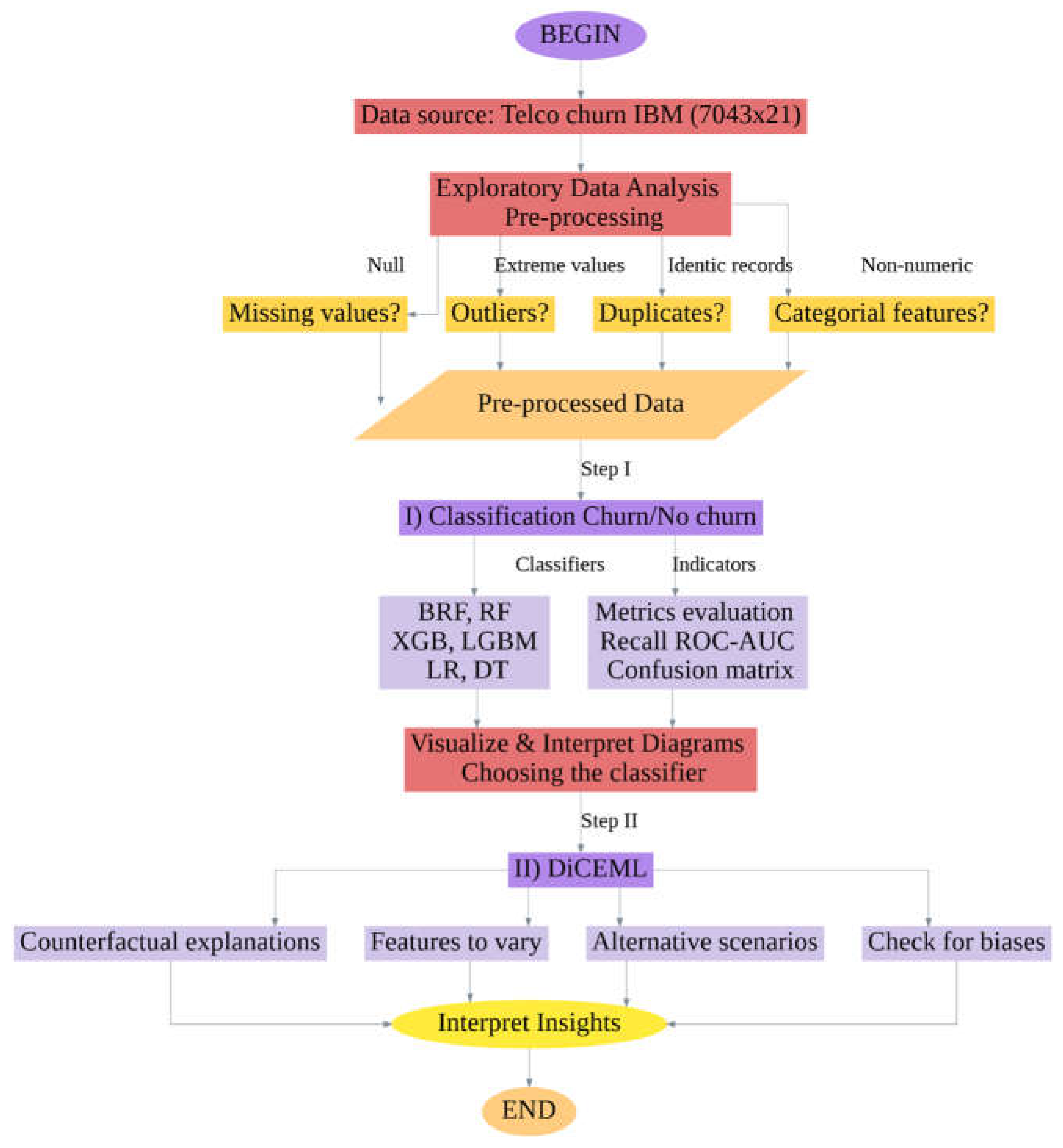
Figure 4 illustrates a workflow focused on predicting customer churn using the IBM Telco Churn dataset, which contains 7043 rows and 21 features.

The process begins by loading the dataset and moving into Exploratory Data Analysis (EDA) and data pre-processing and transformation. During this phase, the workflow checks for potential issues such as missing values, outliers, duplicate records and categorical (non-numeric) features. The first major step involves classifying customers into two categories: churn or no churn. A hyperparameter optimization process using Grid Search combined with 5-fold cross-validation was performed to identify the best-performing configuration for each classifier. This ensured a balanced trade-off between model complexity and generalization performance.

The models are evaluated using performance metrics. Based on these evaluations, the best-performing classifier is selected.

The second major step in the workflow introduces DiCEML. It focuses on explainability and ethical considerations. It explores CF explanations to identify what minimal changes in a customer’s features could lead to a different churn outcome. It also determines which features are most suitable to vary, simulates alternative scenarios and checks the model for potential biases. Finally, insights are interpreted from the analyses, leading to actionable decisions. This flowchart combines ML with interpretability techniques to provide explainable churn predictions.

A summary of our methodological pipeline, including the layered approach involving classification, counterfactual reasoning and bias detection, is provided in

Table 7. Methodological pipeline.

Stage	Description	Techniques/Tools Used	Key Outputs
1. Data preparation	Load and preprocess IBM Telco Churn dataset (n = 7043, 21 features)	EDA, data cleaning, encoding, outlier handling	Cleaned and transformed dataset
2. Churn classification	Train ML models to classify customers as churn/non-churn	BRF, RF, XGB, LGBM, LR, DT; Grid Search + 5-fold CV	Trained models; selection based on Recall, F1-score
3. Model evaluation	Evaluate model performance on imbalanced data	Metrics: Accuracy, Precision, Recall, F1, ROC-AUC, Confusion Matrix	Performance comparison; BRF selected (Recall = 0.72)
4. Counterfactual generation	Generate minimal actionable changes to reverse churn prediction	DiCEML (MILP-based CF generation)	Counterfactual instances X′ = X + ΔX
5. Actionability constraints	Apply business constraints to ensure feasible changes	Feature-level rules (e.g., no gender change, valid categories)	Feasible CFs (e.g., ∆x_contract, ∆x_monthly)
6. Bias detection	Assess fairness across sensitive attributes	Disparate Impact (DI), Selection Rate (SR)	Identification of model biases (e.g., DI < 0.8)
7. Interpretation and recommendations	Interpret CFs and fairness metrics for decision-making	Scenario simulation, feature influence ranking	Actionable retention strategies, ethical insights

.

4. Results

In a customer churn classification problem, recall is generally more important than precision, though the choice depends on the business objectives. Churn detection is a high-stakes problem in business as missing a churner (false negative) means losing a customer, which is costly [38]. Therefore, businesses prefer to act on potential churners.

From a recall point of view in

Table 8. Classification metrics.

	Accuracy	Recall	ROC_AUC	Precision	F1 Score
BalancedRandomForest	0.7648	0.7160	0.8424	0.5517	0.7731
RandomForest	0.7894	0.4843	0.8325	0.6511	0.7787
XGBoost	0.7913	0.5174	0.8365	0.6443	0.7836
LightGBM	0.8031	0.5296	0.8479	0.6756	0.7950
LogisticRegression	0.8112	0.5679	0.8589	0.6834	0.8053
DecisionTree	0.7416	0.5017	0.6663	0.5255	0.7397

, the BRF model has the highest recall score at 0.7160, meaning it is the best at capturing true churn cases. This is expected, as it is specifically designed to handle class imbalance, which is common in churn datasets. Although it has lower precision (0.5517), its strong recall makes it valuable if the goal is to catch as many churners as possible, even at the cost of more false positives.

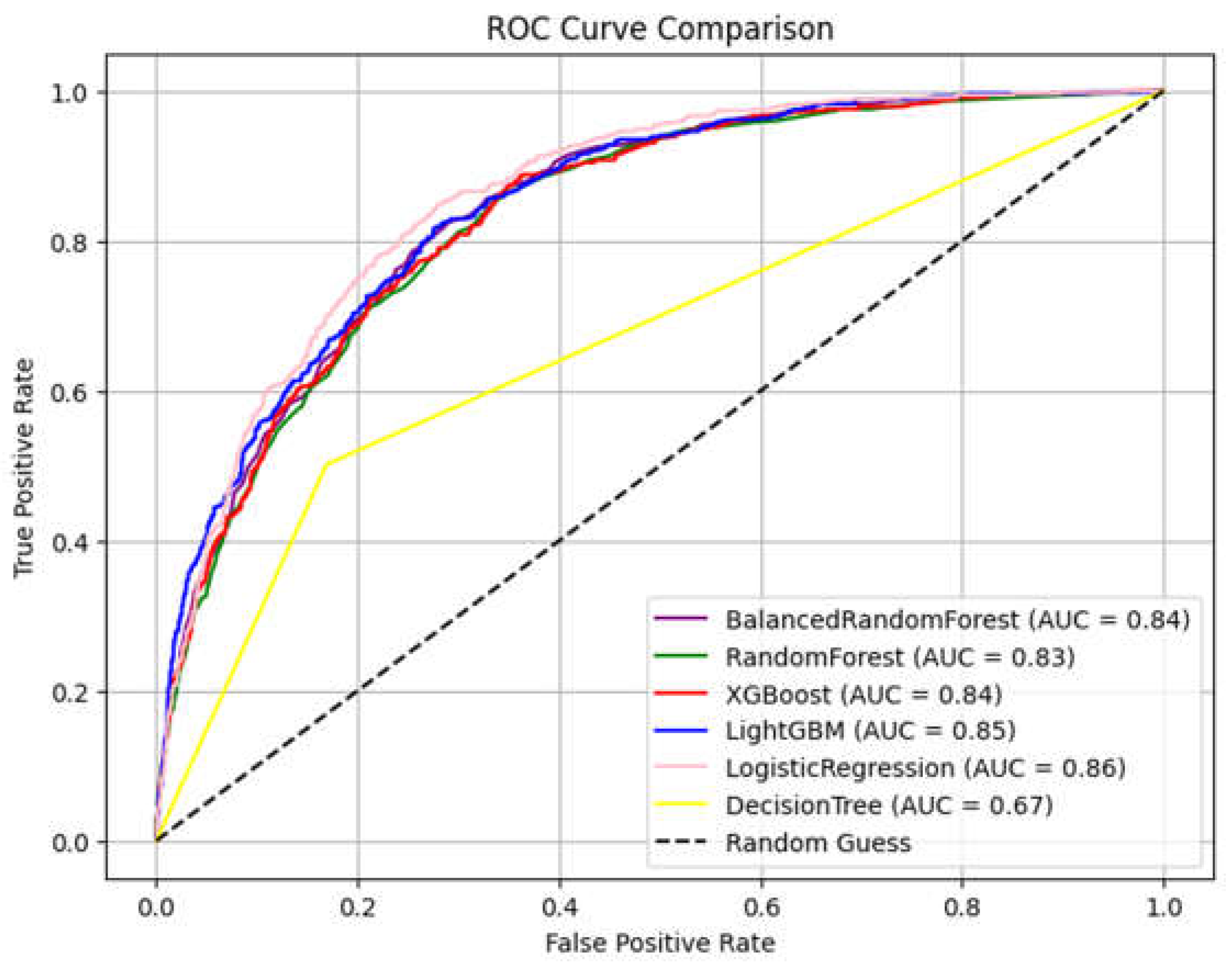
The six confusion matrices in Figure 5 provide a visual breakdown of how each model classifies churned and non-churned customers. LR has the highest AUC at 0.86, showing it has the strongest overall ability to separate churn from non-churn cases (Figure 6). LGBM follows closely with an AUC of 0.85, suggesting it also performs very well in general classification tasks (as in Figure 6). BRF and XGB both achieve an AUC of 0.84, which confirms their reliability, particularly BRF given its earlier high recall (identifying the highest number of churners: 411). RF slightly lags with an AUC of 0.83, but still performs competitively. DT, with an AUC of only 0.67, performs noticeably worse than the ensemble and logistic models, making it the weakest classifier.

Table A1. Hyperparameter tuning via Grid Search (5-fold cross-validation).

Classifier	Hyperparameter	Search Space/Selected Value
Balanced Random Forest	n_estimators	[100, 200, 300]
	max_depth	[None, 10, 20]
	max_features	[‘sqrt’, ‘log2’]
	bootstrap	[True]
	Selected Config	n_estimators = 200, max_depth = None, max_features = ‘sqrt’
Random Forest	n_estimators	[100, 200, 300]
	max_depth	[None, 10, 20, 30]
	max_features	[‘sqrt’, ‘log2’]
	Selected Config	n_estimators = 200, max_depth = 20, max_features = ‘sqrt’
XGBoost	n_estimators	[100, 200]
	max_depth	[3, 5, 7]
	learning_rate	[0.01, 0.1, 0.2]
	subsample	[0.8, 1.0]
	colsample_bytree	[0.8, 1.0]
	Selected Config	n_estimators = 100, max_depth = 5, learning_rate = 0.1, subsample = 0.8
LightGBM	n_estimators	[100, 200]
	max_depth	[5, 10, −1]
	learning_rate	[0.01, 0.1]
	num_leaves	[31, 50, 100]
	min_child_samples	[20, 30]
	Selected Config	n_estimators = 200, learning_rate = 0.1, num_leaves = 31, max_depth = −1
Logistic Regression	penalty	[‘l1’, ‘l2’]
	C	[0.01, 0.1, 1, 10]
	solver	[‘liblinear’]
	Selected Config	penalty = ‘l2’, C = 1, solver = ‘liblinear’
Decision Tree	max_depth	[None, 10, 20, 30]
	min_samples_split	[2, 5, 10]
	min_samples_leaf	[1, 2, 4]
	Selected Config	max_depth = 20, min_samples_split = 2, min_samples_leaf = 1

, which summarizes the hyperparameter settings and search space used for each classifier, based on a Grid Search with 5-fold cross-validation, is provided in Appendix A.

Among the six machine learning models tested, the BRF classifier stood out for its ability to detect churners accurately, achieving a recall score of 0.716. This means it successfully identified nearly 72% of all customers who eventually left, an essential advantage in business settings, where the cost of losing a customer often far exceeds the cost of preventive action.

Table 9. Churn instance from the test set (the first 10 features).

Gender	SeniorCitizen	Partner	Dependents	Tenure	PhoneService	PaperlessBilling	MonthlyCharges	TotalCharges	MultipleLines_No
0	1	0	0	3.0	1	1	79.4	205.05	0

and

Table 10. Churn instance from the test set (the last 10 features).

StreamingMovies_No Internet Service	StreamingMovies_Yes	Contract_Month-to-Month	Contract_One Year	Contract_Two Year	PaymentMethod_Bank Transfer (Automatic)	PaymentMethod_Credit Card (Automatic)	PaymentMethod_Electronic Check	PaymentMethod_Mailed Check	Churn
0	0	1	0	0	0	0	1	0	1

show an original churn instance from the test set. This represents a single customer (test instance) who churned (Churn = 1). Its attributes are:

• gender: 0 → possibly “Female” (depends on encoding)
• SeniorCitizen: 1 → the person is a senior
• Partner: 0 → no partner
• Dependents: 0 → no dependents
• tenure: 3 months → a new customer
• PhoneService: 1 → has phone service
• PaperlessBilling: 1 → uses paperless billing
• MonthlyCharges: 79.4 → relatively high
• TotalCharges: 205.05 → aligns with short tenure

Including the previous categorical dummies that were converted by get_dumies method, the following attributes are added:

• StreamingMovies_Yes = 1 → uses streaming movies
• Contract_Month-to-month = 1 → high-risk contract type
• PaymentMethod_Electronic check = 1 → commonly linked to higher churn

This profile reflects a high-churn-risk customer: low tenure, high monthly charges, a month-to-month contract and electronic check payment.

Table 11. Feature to vary—churn instance from the test set.

PaperlessBilling	MonthlyCharges	OnlineSecurity_Yes	OnlineBackup_Yes	DeviceProtection_Yes	TechSupport_Yes	StreamingTV_Yes	StreamingMovies_Yes	Contract_One Year	Contract_Two Year
1	79.4	0	1	0	0	0	0	0	0

shows several features to vary. These are the features the CF explanation generator is allowed to change to find a non-churn (Churn = 0) outcome: billing method, monthly charges, some services (OnlineBackup, Streaming) and contract type. These are realistic actionable features a business could target (e.g., switch the customer to a yearly contract, offer discounts, enable online backup).

Table 12. CF explanations and features to vary.

PaperlessBilling	MonthlyCharges	OnlineSecurity_Yes	OnlineBackup_Yes	DeviceProtection_Yes	TechSupport_Yes	StreamingTV_Yes	StreamingMovies_Yes	Contract_One Year	Contract_Two Year
0	55.61	0	1	0	0	0	0	0	1
0	55.61	0	1	0	0	0	0	0	1
0	65.93	0	1	0	0	0	0	0	1
1	37.98	1	1	0	0	0	0	0	1

shows four CF explanation examples. These are examples of new feature combinations that would lead the model to predict non-churn (Churn = 0). They show possible minimal changes to flip the outcome. One example CF explanation (row 1) indicates the following changes:

• PaperlessBilling: changed from 1 → 0 (switch to paper billing)
• MonthlyCharges: lowered from 79.4 → 55.61
• Contract_Two year: flipped from 0 → 1

These minimal but strategic changes lead to a non-churn prediction. All four CF explanations maintain the following: OnlineBackup_Yes = 1, No need to activate other streaming services. These suggestions suggest that contract length and lower monthly charges are critical churn drivers.

Table 13. Diverse CF s explanation et (Changed features: PaperlessBilling, MonthlyCharges).

Gender	Senio Citizen	Partner	Dependents	Tenure	PhoneService	PaperlessBilling	MonthlyCharges	TotalCharges	MultipleLines_No
-	-	-	-	-	-	0.0	55.61	-	-
-	-	-	-	-	-	0.0	55.61	-	-
-	-	-	-	-	-	0.0	65.93	-	-
-	-	-	-	-	-	-	37.98	-	-

and

Table 14. Diverse CF set (Changed features: Contract_Two year, Churn).

StreamingMovies_No Internet Service	StreamingMovies_Yes	Contract_Month-to-Month	Contract_One Year	Contract_Two Year	PaymentMethod_Bank Transfer (Automatic)	PaymentMethod_Credit Card (Automatic)	PaymentMethod_Electronic Check	PaymentMethod_Mailed Check	Churn
-	-	-	-	1.0	-	-	-	-	0.0
-	-	-	-	1.0	-	-	-	-	0.0
-	-	-	-	1.0	-	-	-	-	0.0
-	-	-	-	1.0	-	-	-	-	0.0

show a diverse CF explanation set. This shows a more diverse and sparse view of the CF explanations, where only the changed features are shown (others are left as -). For example, at row 1, only PaperlessBilling = 0 and MonthlyCharges = 55.61 are changed, with Contract_Two year = 1. All rows lead to a new prediction of Churn = 0. Diverse CF explanations help provide different pathways to avoid churn, which is useful for customer retention strategies.

Despite reducing the MonthlyCharges from 79.4 to 55 (a significant cost-saving) and activating both OnlineBackup and OnlineSecurity services for the customer, the BRF model still predicts churn (class 1), with a 66% probability. This suggests that even after proactive retention strategies, such as lowering costs and enhancing service offerings, this particular customer still shows a strong tendency to leave. A churn probability of 0.66 means the model estimates that there is a 66% chance that this customer will churn based on their profile and the updated features.

With the MonthlyCharges adjusted from 79.4 to 69 (a modest reduction), OnlineBackup and OnlineSecurity, and switching the customer to a two-year contract, the prediction model now predicts that the customer will not churn (class 0), and the churn probability has dropped to 49%, just below the 0.50 threshold used for classification. This means the customer is now more likely to stay, although the prediction is borderline, suggesting mild retention rather than strong loyalty.

The change that made the difference is extending the contract to two years. We noticed that customers with longer contracts had significantly lower churn rates. Combined with a moderate price drop and added security/backup features, this strategy pushed the model’s confidence just enough to classify the customer as retained. Business could further test contract length variations or add TechSupport to reduce the churn probability even more. If our goal is to minimize risk, aiming for a churn probability below 0.3 or 0.2 may be preferable.

The DI results are presented in

Table 15. DI values for several features.

Feature	DI Value	Interpretation
Gender	0.997	No significant bias; nearly equal selection rates.
SeniorCitizen	0.529	Potential bias; one group (likely senior citizens) is selected much less often than the other.
Partner	0.543	Potential bias; individuals with/without a partner have significantly different selection rates.

. Gender (0.997) → No bias, meaning that both genders receive similar treatment in the model. SeniorCitizen (0.529) → Bias was detected. A DI of 0.529 means that senior citizens (or non-senior citizens) are selected half as often as the other group. This indicates age-related bias in predictions. Partner (0.543) → Bias was detected. If DI is 0.543, it suggests that being in a relationship (or not) significantly affects selection rates. This could be problematic if the model is making unfair decisions based on relationship status.

Beyond prediction, the methodology’s real strength lies in its actionability through CF explanations. For example, for a customer predicted to churn, the model might suggest a small set of feasible changes, such as lowering their monthly fee or switching them to a longer contract, which would have led to a different outcome (i.e., retention). In one test case, even significant reductions in monthly charges and enhanced service offerings were not enough to change the predicted outcome. However, when the customer’s contract was extended from month-to-month to a two-year term, the churn prediction dropped below the decision threshold. This illustrates how certain changes, particularly those that signal long-term commitment, can have a strong impact on customer loyalty.

From a business standpoint, these insights can inform targeted retention campaigns, where interventions are not only personalized but also cost-effective.

Lastly, the framework incorporates a fairness audit to ensure that predictions are ethically sound and unbiased. Disparate Impact (DI) analysis revealed that the model treated male and female customers fairly (DI ≈ 0.997) but showed potential biases against seniors and those without partners. These results signal the need for ongoing monitoring and potential adjustments to ensure equitable treatment across demographic groups, especially in customer-facing decision systems.

The DI values indicate that customers who are senior citizens or do not have partners were less likely to receive favorable outcomes (i.e., being classified as non-churners) compared to their counterparts. This imbalance raises important ethical concerns. If left unaddressed, such biases may lead to systematic disadvantages, such as fewer retention efforts targeted at these groups, less favorable contract offers or even reduced customer engagement. This suggests that the algorithm may be disproportionately classifying these customers as likely to churn, potentially leading to fewer retention efforts directed toward them. Such disparities raise important ethical concerns. If businesses act on model predictions without deeper scrutiny, they may inadvertently neglect or disadvantage certain demographic groups. For example, customers who are older or living alone might be excluded from special offers, loyalty programs or personalized outreach campaigns. This could not only exacerbate existing inequalities but also damage customer trust and expose businesses to reputational risks.

To mitigate these risks, businesses must adopt a more deliberate approach to fairness in predictive modeling. Ethical model development should begin with regular audits of model outputs to monitor for signs of disproportionate impact across demographic groups.

The proposed methodology demonstrates superior performance over traditional explainable AI methods such as SHAP and LIME by not only identifying why a customer is likely to churn but also providing actionable guidance on how to prevent it. While SHAP and LIME excel at feature attribution, explaining which variables contribute most to a prediction, they do not offer concrete recommendations for altering the outcome. In contrast, our methodology integrates DiCEML to generate realistic, diverse and business-constrained interventions that can flip a churn prediction to a retention outcome. These counterfactuals provide strategic insights (e.g., switching to a two-year contract, lowering monthly charges) that are directly usable by customer retention teams. Furthermore, the framework incorporates fairness auditing through DI analysis, which is not natively supported in SHAP or LIME. It ensures that the proposed methodology is interpretable and actionable.

Future work could also (a) investigate feature importance by checking if “SeniorCitizen” and “Partner” play a disproportionately large role in model decisions; (b) examine selection rates per category or look at raw numbers to understand which group is disadvantaged; and (c) test the proposed methodology on loan prediction in the finance industry.

5. Theoretical and Practical Implications

Our research offers several important contributions to both the theoretical foundations of explainable artificial intelligence and its practical implementation in customer churn management. On a theoretical level, the research advances the field of counterfactual reasoning by integrating DiCEML with high-recall classifiers such as the Balanced Random Forest. Unlike traditional counterfactual methods, which often neglect real-world applicability, DiCEML explicitly incorporates business constraints, ensuring that the generated explanations are both realistic and actionable. This approach represents a significant evolution in counterfactual generation, as it addresses the gap between theoretical model interpretability and operational decision-making.

Furthermore, the inclusion of fairness evaluation through Disparate Impact (DI) adds a critical ethical dimension to the framework. By quantifying potential bias in features such as age and relationship status, the methodology contributes to the concept of interpretability and fairness being interconnected, rather than isolated, objectives. In addition, the research introduces a dual interpretability framework, combining local-level, instance-specific explanations with global pattern discovery. This allows the aggregation of individual counterfactual insights to inform broader business strategies, creating a cohesive view that enhances transparency at multiple levels of analysis.

From a practical perspective, the methodology provides direct value to businesses seeking to reduce customer attrition. The counterfactual explanations generated by DiCEML identify minimal and feasible changes, such as adjusting the contract type or offering targeted discounts, that companies can implement to prevent churn. These insights enable highly personalized retention strategies, aligning business actions with the unique characteristics of each customer. Additionally, by focusing on minimal interventions, the approach ensures cost efficiency, helping companies allocate retention resources more effectively and avoid unnecessary expenditure on low-impact measures.

The proposed methodology also supports human-centric decision-making. Since the counterfactuals are both interpretable and grounded in real-world constraints, they can be integrated into sales, marketing or customer support processes, enhancing the ability of personnel to make informed decisions.

6. Conclusions

In business contexts such as customer churn prediction, the primary objective is to accurately identify customers at risk of leaving, allowing businesses to intervene before the loss occurs. In this scenario, recall becomes more critical than precision, since missing a churner (false negative) may result in losing a valuable customer, which is significantly more costly than mistakenly flagging a non-churner (false positive). Businesses are generally willing to act on potential churners, even if it means offering incentives or personalized outreach to some customers who may not have left, because the cost of retention efforts is often outweighed by the cost of customer loss.

Based on the analyses carried out in this paper, the answers to the four research questions (RQs) are as follows:

RQ1: 

How can DiCEML be used to generate realistic and diverse CF explanations for churn predictions under business constraints?

DiCEML generates realistic and diverse CF explanations by identifying minimal, actionable feature changes that shift a prediction from churn to non-churn. It takes into account predefined business constraints by only modifying features that are deemed changeable (e.g., billing method, contract type, service activation and pricing). The system ensures feasibility by not suggesting unrealistic or impractical changes. The results demonstrate how DiCEML produces multiple CF examples, offering varied yet plausible interventions like lowering monthly charges, switching to paper billing or converting to a two-year contract.

RQ2: 

To what extent can these explanations support targeted and effective customer retention strategies in real-world settings?

The CF explanations provide specific, actionable strategies that businesses can deploy to reduce churn risk. For instance, they suggest offering a two-year contract, reducing monthly fees or enhancing service packages like OnlineBackup or TechSupport. These recommendations allow for personalized retention campaigns that are customized to individual customer profiles.

RQ3: 

How do the explanations generated by DiCEML compare to those from other XAI techniques in terms of interpretability, feasibility and actionability?

Compared to traditional XAI methods like SHAP and LIME, which focus on explaining why a prediction was made (feature attribution), DiCEML explains how to change the outcome, making it more actionable. SHAP might show that the contract type and monthly charges heavily influence churn, but DiCEML provides exact changes (e.g., “switch to a two-year contract and lower charges to $55”) to retain a customer. In terms of feasibility, DiCEML takes into account business constraints, unlike SHAP/LIME which might highlight influential features that businesses cannot alter (e.g., age, gender).

RQ4: 

Can DiCEML effectively expose and mitigate biases embedded in the churn prediction models?

DiCEML can be used to audit fairness by examining Disparate Impact (DI) values across demographic features. In our research, it uncovered potential biases in features like SeniorCitizen (DI = 0.529) and Partner (DI = 0.543), indicating that these groups were treated unequally by the prediction model. While gender showed no bias (DI = 0.997), the low DI values for other features suggest age and relationship status biases, which may lead to unfair outcomes. By identifying these disparities, DiCEML supports bias detection and mitigation, guiding model adjustments, reweighting strategies or more representative sampling.

The results of the prediction offer insights into the trade-offs between classification performance metrics. The BRF model emerges as the most effective for capturing true churn cases, achieving a recall score of 0.716. This high recall makes it especially suitable for churn detection, where the aim is to minimize false negatives. While the BRF model has a lower precision of 0.5517 compared to other models such as LGBM or LR, its strength in identifying actual churners makes it valuable when the business goal is to maximize intervention coverage. LR and LGBM, while achieving higher overall classification scores with AUCs of 0.8589 and 0.8479, respectively, exhibit lower recall rates, indicating that they may overlook more at-risk customers. DT, with a considerably lower AUC of 0.6663, shows weak performance in distinguishing between churners and non-churners, making it the least reliable model for this task.

While classification models can flag which customers are likely to churn, their practical value increases significantly when combined with actionable insights. This is where CF explanations show their importance. The CF analysis explores which minimal and realistic changes in the customer’s profile could convert the churn prediction into a non-churn outcome. In our tests, among the actionable changes were a reduction in monthly charges, switching from paperless to paper billing, and most notably, moving the customer from a month-to-month to a two-year contract. These changes alone led the model to reclassify the customer as a non-churner.

Interestingly, scenarios where services like OnlineBackup and OnlineSecurity were activated, without addressing the contract length, did not reduce the predicted churn probability below 50%. In fact, even after offering additional services and lowering the cost from 79.4 to 55, the churn probability remained high at 66%. However, when the customer was moved to a two-year contract with a modest cost reduction and additional services, the model’s churn prediction dropped to 49%. Although borderline, this subtle shift illustrates the disproportionate influence that contract length has on churn predictions and potentially on customer loyalty. This insight enables businesses to prioritize contract offerings and pricing structures in their retention strategies. For more robust interventions, companies could test additional measures, such as offering tech support or larger discounts, aiming to reduce churn probabilities to even safer thresholds, such as below 30%.

The dataset used in our research originates from the telecommunications sector and reflects customer behavior patterns specific to this industry. As such, the dataset may exhibit a certain degree of homogeneity, with customers sharing similar contract types, service options and usage profiles. This homogeneity could limit the generalizability of the model to more diverse customer bases or industries with broader variability in customer characteristics (e.g., variable transaction types or account hierarchies in finance).

While our approach was validated on customer churn in the telecom domain, the underlying framework, combining classification, counterfactual reasoning (DiCEML) and fairness auditing, is generalizable. For instance, in the finance industry, similar models could be employed to predict loan default or credit card cancellation, where DiCEML could recommend actionable policy adjustments (e.g., lowering interest rates, changing repayment terms) while also ensuring fair treatment across demographics. In e-commerce, the methodology could be adapted to predict customer attrition or cart abandonment, with counterfactuals suggesting price adjustments, promotional offers or delivery incentives that could prevent churn. Nonetheless, applying the method to these domains would require domain-specific feature engineering and the careful incorporation of industry-relevant constraints into the counterfactual explanation process. Furthermore, fairness considerations may vary depending on the regulatory context (e.g., stricter fairness compliance in finance), necessitating additional auditing mechanisms.

In future work, we plan to validate the generalizability and consistency of our methodology on larger and more diverse datasets (like loan prediction) or through the use of bootstrapping techniques to simulate multiple training subsets. This will allow us to more thoroughly assess the stability of model performance across varying data configurations.