Abstract
In cross-border e-commerce, effective marketing resource allocation is crucial due to the complexity introduced by diverse product categories, regional differences, and competition among category managers. Current methods either overlook these constraints or fail to enforce them efficiently due to computational challenges. We propose a two-stage optimization framework that integrates predictive models with constrained optimization. In the first stage, predictive models estimate user purchase probabilities and determine upper bounds on product-specific sending volumes. In the second stage, the resource allocation problem is formulated as a large-scale integer programming model, which is then transformed into a minimum-cost flow problem to ensure computational efficiency while preserving solution optimality. Experiments on real-world data show that our framework significantly outperforms baseline strategies, achieving a 14.48% increase in order volume and revenue improvements ranging from 0.19% to 43.91%. The minimum-cost flow algorithm consistently outperforms the greedy approach, especially in large-scale instances. The proposed framework enables scalable and constraint-compliant marketing resource allocation in cross-border e-commerce. It not only improves sales performance but also ensures strict adherence to operational constraints, making it well-suited for large-scale commercial deployment.
1. Introduction
Product push in e-commerce refers to the proactive delivery of promotional messages to users via subscription channels such as emails and text messages. Based on functional differences, push notifications can be categorized into transactional and marketing types. The former includes notifications related to orders, payments, and logistics, whereas the latter focuses on product recommendations and promotional campaigns. The primary push channels include in-app notifications, emails, and web pop-ups [1]. Figure 1 illustrates common push notifications in an e-commerce context.

Figure 1.
Examples of push notifications in e-commerce.
Push notification marketing, a cornerstone revenue driver in e-commerce ecosystems, has proven effective in amplifying brands and increasing sales while maintaining exceptional cost efficiency [2]. Empirical evidence from Campaign Monitor shows that email marketing achieves an industry-leading return on investment (ROI) of $42 for every $1 invested [3]. This metric is particularly relevant given the structural similarities between email and push notification systems. This economic advantage is substantiated by operational data from cross-border e-commerce company B, where push notifications generate 14% of total sales revenue at a marginal cost below 0.01 pence per message—a finding consistent with Goic et al.’s econometric analysis [4].
Push notification marketing plays a crucial role in enhancing marketing effectiveness across various scenarios. For example, during the summer season, businesses can leverage push notifications to promote seasonal products with exclusive discounts to attract customers. Moreover, personalized push notifications help strengthen user engagement [5]. Research shows that when users perceive push notifications as valuable, their brand loyalty and willingness to recommend significantly increase [6]. However, with rising customer acquisition costs in e-commerce, an indiscriminate push strategy can lead to a negative cycle of “high acquisition cost—low user retention” [7].
In cross-border e-commerce, market conditions exhibit substantial heterogeneity across countries due to factors such as geographic location, seasonal variations [8], and consumer preferences [9]. Consequently, the demand distribution for hot-selling product categories varies significantly across regions. For instance, outdoor equipment tends to experience higher demand in European markets, whereas consumer electronics are particularly popular in Southeast Asia. To enhance operational efficiency, cross-border e-commerce platforms typically adopt a category-based management structure, wherein each product category is overseen by a dedicated category manager [10]. However, within this framework, user attention constitutes a limited resource, often becoming the focal point of competition among category managers. In pursuit of higher sales performance, category managers may independently allocate excessive advertising budgets, leading to an oversaturation of product promotions that disrupts user experience [11,12]. Such uncoordinated competition not only reduces the efficiency of advertising budget utilization but also negatively impacts user engagement and, ultimately, compromises overall revenue. Therefore, an effective marketing resource allocation strategy should account for product-specific demand patterns, allocate advertising budgets in a data-driven manner, and employ a centralized optimization approach to maximize overall efficiency, rather than allowing decentralized competition among category managers.
Existing research on marketing resource allocation can be broadly classified into two methodological paradigms: the two-stage method and the end-to-end method [13]. In the two-stage method, user purchase probability is first forecasted, followed by an optimization model that determines marketing resource allocation. However, conventional optimization models largely overlook competitive interactions among category managers, potentially resulting in inefficient budget allocation and suboptimal marketing effectiveness. End-to-end methods integrate prediction and optimization into a unified framework, theoretically yielding superior results. Nevertheless, in the context of cross-border e-commerce, complex operational constraints [14], such as budget limitations, render many end-to-end methodologies theoretically infeasible. To bridge this research gap, we refine the two-stage approach by incorporating these domain-specific constraints into the optimization framework. This refinement not only improves the overall efficiency of marketing resource allocation but also enhances user experience by mitigating redundant advertising exposure.
The primary contribution of this study is the development of a structured two-stage optimization framework that explicitly integrates key constraints inherent to cross-border e-commerce: (a) inter-category marketing resource equilibrium, ensuring a balanced allocation of marketing resources across different product categories; (b) user fatigue modeling under multi-product advertising exposure, capturing diminishing engagement due to excessive promotional frequency. Our framework retains all hard constraints. Secondly, we address the computational complexity of the Multi-Category Multiple Knapsack Problem (MCMKP) [15] by reformulating it as an equivalent Minimum-Cost Flow (MCF) network. This transformation enables an exact solution with polynomial-time complexity guarantees, significantly improving scalability and making the proposed approach practical for large-scale deployment in real-world marketing resource allocation.
2. Related Work
Extensive research on product push notifications spans marketing, management science, and machine learning [16]. This section reviews marketing resource allocation methods in e-commerce push systems, categorizing existing approaches into two-stage optimization and end-to-end optimization paradigms.
Traditional push strategies predominantly employ customer segmentation [17,18] and contextual differentiation frameworks [19]. The Recency-Frequency-Monetary (RFM) model [20] exemplifies threshold-based notification triggering mechanisms. While offering operational simplicity and interpretability, such methods fail to achieve global resource optimization under multi-constraint scenarios. Consequently, data-driven approaches have gained prominence [21]. Amazon’s product-based collaborative filtering [22] exhibits limitations as it tends to generate repetitive recommendations, potentially inducing user fatigue. The Look-alike algorithm [23], a user-similarity-based collaborative filtering method [24], expands target audiences but relies heavily on sufficient seed user data and performs optimally for mainstream products. Gao et al. [25] proposed an adaptive push method at Yahoo, leveraging user-news vector interactions to train a click-through rate (CTR) model. The system triggers notifications if the estimated click probability exceeds a predefined threshold. However, due to data sparsity, accurately estimating these probabilities remains challenging, often leading to conservative thresholds that reduce push coverage.
The two-stage optimization paradigm [26] remains prevalent in marketing resource allocation. In the first stage, machine learning models predict individual treatment effects, employing techniques such as causal forests [17] and representation learning [19]. While standard machine learning objectives do not explicitly incorporate downstream optimization tasks, empirical studies have demonstrated the practical effectiveness of the two-stage framework [27]. However, current two-stage methods often do not fully align with the specific needs of cross-border e-commerce in the second-stage modeling. For instance, Yuan [28] employed a Multinomial Logit Model to predict user interest probabilities, subsequently formulating the problem as a Multiple Choice Knapsack Problem (MCKP). Our problem setting more closely aligns with the MCMKP, necessitating a more sophisticated optimization approach. Lu et al. [29] considered different customer segments and incorporated similarity constraints into their model to ensure that marketing actions or outcomes are similar across different customer groups, thereby avoiding unfairness. However, in our problem, customers are highly heterogeneous, and we need to tailor marketing constraints according to different regions.
Existing two-stage methods for marketing resource allocation face another critical limitation in handling large-scale optimization problems. When dealing with massive customer bases, many second-stage models compromise solution quality by either relaxing constraints or employing heuristic algorithms to accelerate computation. For instance, Javier et al. [30] first employed uplift modeling to estimate conditional average treatment effects, then solved an online multiple-choice knapsack problem to obtain approximate solutions. Baardman et al. [31] formulated dynamic promotion targeting as a nonlinear mixed-integer programming problem and developed an adaptive greedy algorithm to solve it. While their approach achieved approximately 7% average revenue improvement in large-scale instances, such heuristic methods cannot guarantee optimality. While Wang et al. [32] demonstrated a 99% optimality ratio between Lagrangian dual and linear programming solutions for bonus allocation; their results hold only under simplified constraints (single global budget and uniform per-user limits) that differ fundamentally from our setting with multiple interdependent constraints. These examples collectively illustrate the persistent efficiency-quality tradeoff in two-stage frameworks.
End-to-end methods address stage-wise inconsistencies by integrating prediction and optimization into a unified framework. These approaches typically relax discrete decision variables into continuous spaces and construct differentiable loss functions using techniques such as analytical smoothing [33] and stochastic perturbation [34]. The Smart Predict-then-Optimize (SPO) framework [35] proposes to jointly train the prediction and optimization problems simultaneously without relaxing constraints. However, its applicability is limited to cases where parameters appear linearly in the objective function, a condition violated in our constraint structure. In our setting, the maximum sending volume of products appearing in constraints is also estimated. Furthermore, some methods transform the optimization problem into a dual problem and perform joint optimization. However, this approach is only feasible when all customer constraints are identical, which is not applicable in our problem. Zhou et al. [36] transformed budget constraints into a dual problem, incorporating user reception limits into the objective function to eliminate explicit constraints. Similarly, Yan et al. [37] converted the optimization problem into a dual problem and incorporated the optimization objective as a regularizer into the loss function for optimization.
In summary, while existing approaches have advanced marketing resource allocation, they exhibit critical limitations in handling a cross-border e-commerce setting. The current methods either oversimplify the solving algorithm for computational tractability or struggle to incorporate specific constraints in the optimization model. Our work bridges these gaps by developing a novel two-stage framework that considers heterogeneous products with an exact minimum-cost flow optimization, uniquely capable of handling multiple constraints while maintaining computational efficiency.
3. Methodology
3.1. Problem Definition
According to company B, user interactions with product push notifications are illustrated in Table 1. If users do not open notifications immediately, they can later review them in the notification center or ignore them entirely. Upon opening, if a user is interested in the product, they may proceed to view details and make a purchase. Throughout this process, the number of engaged users gradually declines. According to Company B, approximately 20% of users open push notifications, around 10% click on the content, and about 5% complete a purchase.

Table 1.
User responses to product push notifications.
As illustrated in Figure 2, cross-border e-commerce companies typically adopt a category-based management model, where each product category is managed by a dedicated category manager who formulates independent marketing strategies. For instance, products such as smartphones and earphones fall under the responsibility of the consumer electronics category manager, while items like cycling accessories and camping tents are managed by the outdoor equipment category manager. To maximize the exposure of their respective products, category managers may allocate excessive budgets for their own promotions, resulting in an oversaturation of promotions. Therefore, an effective marketing resource allocation mechanism should systematically consider market demand across different product categories [38].
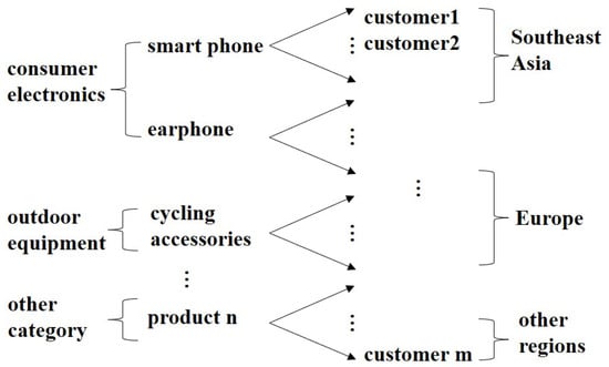
Figure 2.
Company B’s product management framework.
Currently, Company B’s advertising push strategy primarily relies on manual decision-making, where operational staff formulate push notification rules based on experience, such as selecting products aligned with prevailing sales trends and targeting specific user segments. However, rule-based strategies leave considerable room for improvement in terms of open rate and conversion rate. Company B employs a fixed-cycle decision-making mechanism, with each decision cycle lasting approximately seven days. During each cycle, n category managers each select one product for promotion, while the push notification system’s operator is responsible for allocating these n products among m users. Specifically, the operator selects a target subset of users for each product i and delivers push notifications via email, Twitter, or short message service (SMS). Due to message length constraints in certain channels (e.g., Twitter advertisement), each push notification contains only one product. We hypothesize that each push promotion contains only one product. Therefore, if a promotion includes K different products, it is treated as K separate push promotions. This implies that user j may receive up to K promotions, with each promotion containing a single product.
Figure 3 illustrates the decomposition of the product push problem into two sub-problems. Sub-problem 1 is a prediction task: using historical data from time period to , we train a model to estimate user purchase probabilities. Sub-problem 2 is the user allocation problem: based on the predicted probabilities, we formulate an allocation strategy for the time period to , which is subsequently validated through experiments.

Figure 3.
Decomposition of the product push notification into two sub-problems.
In sub-problem 1, we train a predictive model to estimate purchase probability. Specifically, we denote the probability that user j purchases product i upon receiving promotional message k as . We assume that when a user receives multiple promotions in a short period, the effectiveness of subsequent messages diminishes. Thus, is also dependent on the number of promotional messages received (K).
To optimize user-product allocation, we formulate an IP model that accounts for multiple product assignments to a single user. Discussions with business experts and data analysis have identified key constraints that must be incorporated. The optimization framework employs methods such as Cplex [39], minimum-cost flow algorithms [40], and greedy heuristics [41] to determine the best allocation strategy. The model defines product-user assignment decisions as binary variables and maximizes expected sales revenue.
The primary limitation of the IP model lies in computational complexity. Even on mid-sized e-commerce platforms, user bases range from hundreds of thousands to millions, and the number of promoted products exceeds ten. Consequently, the optimization model must handle millions of binary decision variables. This computational burden not only consumes significant resources but may also delay real-time decision-making. To mitigate this, we reformulate the problem as a minimum-cost flow problem, significantly reducing complexity and accelerating computations.
The notations used in this study are summarized in Table 2. Section 3.3 and Section 3.4 provide detailed formulation of the two sub-problems.
Table 2.
Notation and definitions.
3.2. Data Collection
This study collected authentic operational data from Company B’s cross-border e-commerce platform spanning 2021 to 2023, covering three core dimensions: user behavior, product information, and promotion records. The raw data underwent rigorous ETL processing, including de-identification, outlier cleansing, and spatiotemporal alignment. User behavior data was collected through event tracking logs, recording user IDs, session IDs, product IDs, action types (browsing/clicking/cart addition/purchase), and timestamps. Product data was extracted from the enterprise ERP system, comprising 128 products across 16 primary and 32 secondary categories, with feature dimensions including price and categorical hierarchies. Promotion records were obtained from the CRM system, containing push content, recipient information, delivery timestamps, and conversion status.
To ensure privacy protection, sensitive fields (e.g., gender, age) were hashed for encryption. Throughout data collection, we strictly adhered to relevant privacy policies and data protection regulations, implementing comprehensive measures to safeguard data security and user confidentiality.
3.3. Prediction Tasks
3.3.1. Prediction Model Development
The purchase probability of user j seeing product i on the k-th promotion notification is denoted as . This paper models the problem of conversion rate calculation as a binary classification issue: if user j purchases product i, then the user-product pair constitutes a positive instance, labeled as ; if the user has browsed but not made the purchase, then the user-product pair constitutes a negative instance, labeled as . Based on historical data and the characteristics of users and products, the feature vector for product i is denoted as and for user j as [42]. These vectors are combined into a single input sample , forming a new feature vector. Historical data trains a predictive function, the predictive model . After inputting the feature vector into the predictive model, the resulting prediction is:
where represents the learnable parameters obtained through training, and represents our predicted probability of user j purchasing product i, which is used in sub-problem 2, .
According to the purchase state theory [43] and the law of diminishing marginal utility from behavioral economics [44], we assume that excessive exposure to promotions adversely affects user response rates. Therefore, , where , and K represents the maximum number of promotions a user receives. To formalize this hypothesis, we introduce the hyperparameter decay, which quantifies the diminishing effectiveness of subsequent promotions.
As for the experiment setting, 1 July was the starting point, and data from 1 July to 1 August was used to train the prediction models estimating purchase probabilities. Given a collection of products I and a set of users C, with and , the prediction model forecasts for user purchasing item . Three prediction models were employed: logistic regression [45] (LR), eXtreme Gradient Boosting [46] (xgBoost), and the Wide&Deep model [47] (WDL). A comprehensive comparison was conducted to determine the most suitable method for product recommendations in push notifications and to explore potential integration with optimization models.
The maximum number of promotional messages for product i is determined based on historical sales data. Specifically, is calculated as a moving average of product i’s history sales volume, serving as an upper bound constraint to prevent over-promotion.
3.3.2. Feature Selection and Engineering
The product dataset contains information such as product IDs, names, categories, original prices, and discounted prices. Key details include product category and pricing. Although shipping fees influence buying behavior, they were excluded due to complex pricing rules and discrepancies between recorded and actual costs. The product feature details are listed in Table 3.
Table 3.
Product Features.
The user information database includes user ID, country, VIP level, and registration type. Gender and age data were excluded due to accuracy concerns.
The user feature vector, as shown in Table 4, consists of seven features. One is categorical—the user’s country (or region), which impacts currency, shipping, and tax rates. The remaining six numerical features derive from purchase data over the past month, reflecting purchase behavior.
Table 4.
User Features.
Handling categorical variables with high cardinality, such as product categories, requires careful consideration. One-hot encoding creates high-dimensional feature spaces, reducing efficiency and increasing memory usage. Furthermore, sparse data from one-hot encoding makes training difficult and prone to overfitting. To mitigate this, the embedding method maps high-dimensional categorical features into low-dimensional continuous vectors, preserving categorical information while improving efficiency. For example, a third-level category is transformed into a k-dimensional vector.
Feature embedding technology transforms high-cardinality categorical features into dense, low-dimensional vectors. Using PyTorch and the DeepCTR framework [48], the Embedding Layer facilitates feature transformation. During training, optimizing vector representations enhances model performance by strengthening feature relationships. The Embedding Layer converts features into dense vectors, which are input into the neural network and continually updated during training to achieve optimal representations.
3.3.3. Evaluation Metrics
We evaluate our work through the following indicators: accuracy, precision, recall, F-value and area under the receiver operating characteristic curve (AUC).
Accuracy is given by:
Precision is given by:
Recall is given by:
The F-value is a comprehensive index, which is the harmonic average of precision rate and recall rate, which are defined as:
where TP is a true positive, TN is a true negative, FP is a false positive and FN is a false negative in the prediction. AUC is the area enclosed by the ROC curve and the coordinate axis. It shows the ability of the model to provide prediction under different decision thresholds, which is one of the indicators to measure the merit of machine learning.
3.4. Promotion Allocation Models and Algorithms
The limited attention resources of users act as a bottleneck for delivering product push notifications. It is essential to allocate users among multiple products simultaneously to optimize the delivery of content across several rounds of product pushes. During to , user allocation was modeled as an Integer Linear Programming problem. Our 0–1 decision variable, , indicates whether product i is sent to user j in the k-th promotion notification. Sub-problem 2 aims to determine the values of . When the optimization goal is to maximize the number of orders, the objective function is the sum of . When maximizing revenue is the goal, the objective function becomes . The objective function of this model can be adjusted based on the real objectives. An example related to sub-problem 2 (when , , , ) is provided in the Appendix A.
During this decision period, the total number of promotional ads that can be sent to all customers should not exceed N. Each product i can be sent to no more than customers during the promotional period. No product can be promoted repeatedly to any customer within each period. Each time a customer sees a product, it counts as one unit of exposure. The promotional ads received by customers must follow a sequential order. That is, the opportunity for a second viewing of promotional ads comes after the first viewing, to align with reality.
Considering the large user base in e-commerce product promotions, obtaining an accurate solution for large-scale integer linear models tends to be time-consuming. Therefore, we transform the integer linear optimization model into a minimum cost flow problem to reduce computational complexity and time. In this sub-problem, it is necessary to ensure the equivalence of the optimal solution obtained by converting the integer linear model to the minimum cost flow. In Section 4.3, we demonstrate that despite having more decision variables, the minimum-cost flow approach offers significant computational advantages over integer programming, particularly for large-scale problems. For instance, it reduces computation time by 87.6% when users exceed 10,000. This method achieves near-greedy algorithmic efficiency while matching the global optimum performance of integer programming. Additionally, we compare this method to the hot-selling strategy as a benchmark and a heuristic greedy algorithm.
3.4.1. Hot-Selling Strategy
In many actual promotional processes, the strategy relies on statistical rules for product recommendations without using advanced models or algorithms. Company B’s prevalent promotion strategy involves pushing products based on the top 3 hot-selling regions. For example, if the historical sales percentages for Product A are highest in Country 1, Country 2, and Country 3, Product A is promoted to users in these countries in sequence. This procedure is repeated for other products. Once the maximum number of promotions for a cycle is reached, the process halts. In practice, Company B does not limit the number of product pushes per user. Section 4.2.2 and Section 4.2.3 compare the hot-selling strategy with other algorithms.
3.4.2. Greedy Rule-Based Algorithm
In real-world product promotion scenarios, given the massive user base, employing an integer linear model often requires significant computational resources to obtain an optimal solution. To expedite the process of finding satisfactory solutions, we propose a heuristic algorithm based on a set of greedy rules.
Differing from the region-based hot-selling approach currently utilized by the company, our greedy optimization algorithm incorporates the following considerations during each round of product promotion.
The number of promoted products accepted by users affects the subsequent acceptance probability of other products. Therefore, the greedy algorithm considers the number of products each user has received, denoted by K, the maximum number of products a user can accept. Additionally, the algorithm accounts for the fact that users’ purchasing probability decreases as the number of promoted products they receive increases. The purchase probability is represented as , where . Each product has a maximum quantity that can be sent. We denote this as , the maximum sending volume for product i. The pseudo-code for the greedy algorithm (GA) is described in the Appendix A.
3.4.3. Integer Programming Model
The probability of purchase, denoted as , is predicted by machine learning models in the first stage and serves as input parameters in the second-stage optimization model. The objective function varies based on the competitive strategy. When the objective is to maximize the number of orders, the function is given by the sum , as shown in Equation (3). To maximize sales amount, the objective is , as shown in Equation (4). For maximizing sales profit, the objective function is , as shown in Equation (5).
The model is subject to operational constraints across three aspects:
- Marketing resource limits:
- User experience:
- 3.
- constraint (9): Single-product promotion. Each promotional message (e.g., the k-th message to user j) contains exactly one product.
- 4.
- constraint (10): Exposure uniqueness. Users receive each product i at most once during the decision period.
- 5.
- constraint (11): Sequential delivery. Promotion in k-th period can be sent to user j only after delivering promotion in -th period. More specifically, the right-hand side equals the number of promotion messages that user j receives before period k; this number must be at least one to allow sending product i to user j in period k.
- Regulatory compliance in logistics:
- 6.
- constraint (12): Certain products may be unavailable in specific regions. For example, in Denmark, some biodegradable plastic products may be prohibited due to environmental regulations.
Building upon these constraints, we now formalize the complete integer programming model. The IP model for optimizing the number of orders is presented below.
3.4.4. Equivalent Minimum-Cost Flow Problem
In e-commerce environments, user counts can be substantial. The case studies in this paper involve approximately 60,000 to 100,000 users, while actual platforms may handle hundreds of thousands or even millions of users. This results in a large number of decision variables in integer linear models, which may require considerable time and computational resources to solve using solvers like Cplex. To reduce computational time while maintaining the optimal solution, we transform the integer linear model into an MCF problem [40,50] and solve it using the successive shortest path algorithm [51].
Figure 4 illustrates the equivalent MCF model [52]. Let S denote the source node with supply N, and T denote the sink node with demand N. The supply constraint ensures that the total number of promotional activities does not exceed the budget N, corresponding to constraint (7) in the IP model. Each unit of flow from S to T represents a promotion sent to a user, and all other nodes have zero supply or demand.
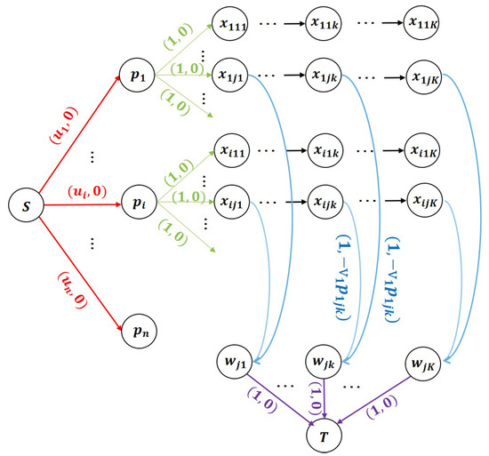
Figure 4.
Equivalent minimum cost flow problem.
Each product i is represented by node , connected to S via a red arc with capacity , ensuring that the number of promotions for product i does not exceed the budget , by constraint (8) in the IP model. The cost per unit flow along this arc is zero.
The green arrowed arc from node to node has a capacity of 1 and zero cost. This ensures that each user receives at most one promotion for each product, fulfilling constraint (10) in the IP model. The decision variables form an matrix for n products and m users, with the j-th row corresponding to user j and the k-th column corresponding to the k-th promotion. Flow between and must pass sequentially as we mentioned in constraint (11), ensuring a logical flow from to .
Blue arrows from to represent binary decision variables with a capacity of 1. These arcs introduce a cost of , where is the product’s value and is the promotion’s expected revenue, representing the negative expected sales revenue. This negative cost ensures that minimizing the total cost corresponds to maximizing expected revenue.
Purple arrows from to T have a capacity of 1 and zero cost, ensuring that each user can receive at most one promotion for each product, in line with constraint (9) in the IP model.
Thus, we transform the IP model into an MCF problem. Unlike standard MCF problems with positive costs, our network features only zero or negative costs. Nevertheless, standard MCF algorithms remain applicable, since there are no negative cycles [53,54] in Figure 4.
The MCF can be considered a special case of a linear model. To ensure that the solutions of the IP and MCF models align, we need to satisfy three conditions: (i) the MCF problem should yield a 0–1 integer solution, (ii) the total sending amount N must be consistent between the IP and MCF models, and (iii) the constraints in the MCF problem must remain valid. These conditions are discussed below.
(i) Feasible integer solutions. The Integrality Theorem [55] ensures that maintaining integer demand and capacity in the MCF model guarantees an optimal integer solution. Since the capacity on edges connecting nodes and is 1, the binary decision variables will take values of 0 or 1, corresponding to integer solutions.
(ii) Total marketing resource limits N. In IP model, constraint (8) enforces the marketing resource limitation through . The monotonicity of coefficients in the objective function guarantees that the optimal solution necessarily activates the binding property, attaining the tight equality . In the MCF model, the flow conservation at each node ensures that N units of flow are directed from S to T. With edge costs strategically parameterized as , the network topology inherently prioritizes high-revenue pathways, ensuring the exact transmission of N flow units. Both methodologies meet constraint (8), where the IP model achieves this through objective-driven boundary activation, while the MCF framework enforces it through topology.
(iii) Constraint 5 Validity. Although constraint 5 is not explicitly present in the MCF model, we demonstrate that the optimal solution in the MCF adheres to this constraint. If a feasible solution does not satisfy constraint 5, we can adjust the decision variables by swapping the k-th and -th promotion assignments without violating other constraints. This adjustment results in a new solution with an equal or better objective value, as shown in Table 5.
Table 5.
Adjustments for a better solution.
4. Experiments and Results
4.1. Experimental Design
We generated multiple instances using a sliding window, each spanning approximately 37 days. The first 30 days served as training data, while the subsequent 7 days were used to validate the allocation effectiveness of predictive models and optimization algorithms. For the allocation task, the optimization objective aimed to maximize the number of orders or sales revenue. Each predictive model (Logistic Regression, xgBoost, and Wide&Deep) was paired with either a greedy algorithm or minimum-cost flow to propose user allocation schemes. The objective value associated with each scheme was then assessed.
As illustrated in Figure 5, we employed a sliding window approach to generate multiple instances. Data on user browsing and purchasing behavior for selected categories was collected from 1 June to 7 November. Taking the first instance as an example, data from 1 June to 30 June was used to generate sample features such as the recent average spending and total discount amount for each user. Then, data from 1 July 2021, to 31 July 2021, was used to train the recommendation model and predict purchase probabilities. These probabilities informed the user allocation schemes for the period from 1 August to 7 August. We compared the actual user allocation schemes with the real purchase occurrences to evaluate the results.

Figure 5.
Sliding time window for generating multiple instances.
In this experiment, the sliding window step size was set to one month, resulting in four total instances. The distribution of these instances is summarized in Table 6. Given that irregular data is common regardless of the collection period, the data preprocessing phase involved excluding missing values, corrupted data, anomalies, and incomplete records.
Table 6.
Time distribution of instances.
The problem was formulated as a binary classification of purchase outcomes. If a customer j purchased product i, the label was set to 1; otherwise, if the customer viewed product i but did not purchase it, was set to 0.
4.2. Experimental Results
We employ different metrics for these two sub-problems. In sub-problem 1, commonly used product recommendation metrics include accuracy, precision, recall, and AUC. In sub-problem 2, objective function values are used as evaluation metrics.
We first present the experimental results of the prediction task. We conduct a comparative analysis of the performance of three predictive models across four instances. We introduce the improvement effects achieved through various combinations of predictive models and algorithms, with a specific focus on optimizing the number of orders and sales revenue separately. All experiments were conducted on an Intel(R) Core(TM) i5-9400F CPU@2.90GHz, with 16.0 GB RAM. The operating system and software platforms used were Windows 10 Professional x64 Edition, PyTorch 1.11.0, and Python 3.8.
4.2.1. Comparison of Predictive Model Performance
In this subsection, we present the predictive performance of three models on the test sets of four instances. We analyze and compare which type of predictive model demonstrates the best overall performance on this dataset. Figure 6 compares the predictive performance of three models across four test instances, showing (a) recall, (b) precision, (c) accuracy, and (d) AUC metrics.
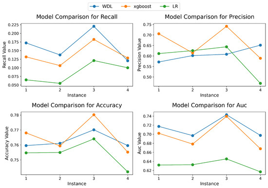
Figure 6.
Performance evaluation of models across 4 instances.
The experimental results reveal significant performance variations among predictive models in cross-border e-commerce scenarios. In terms of recall, the Wide & Deep (WDL) model demonstrates consistent superiority across all four test instances, particularly outperforming XGBoost and Logistic Regression (LR) in Instances 1–3. XGBoost marginally surpasses WDL in Instance 4 (by 0.008). For precision and accuracy metrics, WDL and XGBoost exhibit alternating leadership across instances. In Instance 2, WDL achieves a precision of 0.72 compared to XGBoost’s 0.68, while XGBoost shows reversed dominance in Instance 4 with an accuracy of 0.78 versus WDL’s 0.75. XGBoost’s superior performance in specific instances may stem from efficiently handling high-dimensional sparse features, such as regional preferences in cross-border user behavior. The results indicated that the AUC of the WDL model was the highest, followed by the XGBoost, with the LR exhibiting the lowest AUC value.
In the case of the xgBoost model in instance 1, we analyzed the most crucial features in calculating the purchase probability. Figure 7 displays the 8 most influential features in xgBoost. The top two significant features are the final price of products (final_price) and the user’s historical maximum transaction amount (’products_price’, ’max’). This finding aligns with company B where purchase decisions are primarily driven by price sensitivity and constrained product category preferences.
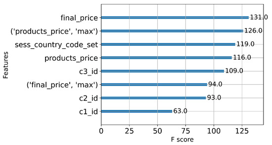
Figure 7.
Top 8 important features in xgBoost.
4.2.2. Comparison of Optimization Effects on Orders
In this section, we analyze the optimization results with the number of orders as the objective. Based on the predictive models (LR, xgBoost, or WDL), we compute the purchase probability . This probability serves as a parameter in the integer linear model presented in Section 3.3. The optimization objective is set to maximize the number of orders: . Subsequently, optimization algorithms (e.g., using Cplex, greedy algorithms, or minimum-cost flow algorithms to solve integer programming problems) are employed to determine the values for the decision variables , thereby obtaining the user allocation scheme for instance 1. We evaluate the comparison between the user allocation strategy derived from our model and the actual purchase situations. For example, if user j indeed purchased item i (i.e., ), and we initiated the promotion (), an order is accomplished. The optimization results for instance 1 are presented in Table 7. The detailed results of the other three instances with the same objective are provided in the Appendix A.
Table 7.
Results of instance 1 with optimization for the number of orders.
Instance 1: In instance 1, the prediction of the purchase rate involved training the predictive models using data from 1 July to 31 July. Among the three predictive models, the WDL model displayed the best performance in terms of the AUC metric. Different strategies, such as regional hot-selling, greedy algorithm, and minimum-cost flow algorithm, were employed to provide user allocation plans from 1 August to 7 August.
The number of orders achieved using the regional hot-selling strategy was 7087; the final optimized number of orders when using the logistic regression model with the greedy algorithm was 7930. The most effective combination of the predictive model and optimization algorithm was the WDL model paired with the minimum-cost flow algorithm, achieving the highest number of orders of 9733. The predictive and optimization combination increased the number of orders by 11.90% to 37.34% in comparison to the regional hot-selling strategy.
When optimizing for the number of orders, predictive models exert a significantly greater impact than the choice of optimization algorithms. The variation in the number of orders resulting from different predictive models can exceed 25%, while the improvement differences from optimization algorithms are only around 6%. Although predictive models dominate the outcome, optimization algorithms further enhance the number of orders by tapping into the demand for long-tail products.
Instance 2: The optimization results for instance 2 is presented in Table A3. The achieved number of orders using the regional hot-selling strategy was 8680. The most effective combination of the predictive model and optimization algorithm was the WDL model paired with the minimum cost flow algorithm, achieving the highest number of orders of 12491. The predictive and optimization combination increased the number of orders by 39.42% to 43.91% in comparison to the regional hot-selling strategy.
Instance 3: The optimization results for instance 3 are presented in Table A5. The achieved number of orders using the regional hot-selling strategy was 9142. The most effective combination of the predictive model and optimization algorithm was the xgBoost model paired with the minimum cost flow algorithm, achieving the highest number of orders, 12358. The predictive and optimization combination increased the number of orders by 7.48% to 35.18% in comparison to the regional hot-selling strategy.
Instance 4: The optimization results for instance 4 is presented in Table A7. The achieved number of orders using the regional hot-selling strategy was 5277. The most effective combination of the predictive model and optimization algorithm was the WDL model paired with the minimum cost flow algorithm, achieving the highest number of orders of 9879. Compared to the hot-selling strategy, the combination of prediction and optimization may reduce the number of orders by −0.99%. However, selecting an appropriate predictive model and algorithm can increase the number of orders by 0.19% to 43.91%. The variation in the number of orders resulting from different predictive models can exceed 35% and the improvement differences from optimization algorithms are around 20%.
4.2.3. Comparison of Optimization Effects on Sales Revenue
In this section, we analyze the optimization results with sales revenue as the objective. The optimization results for instance 1 are presented in Table 8. The detailed results of the other three instances with the same objective are provided in the Appendix A.
Table 8.
Results of instance 1 with sales revenue optimization.
Instance 1: Under the regional hot sales strategy, the sales revenue amount is approximately 590,000. Implementing the logistic regression model in combination with the greedy algorithm resulted in the final optimized sales revenue of around 720,000. The most effective combination involving the WDL model with the minimum-cost flow algorithm led to the highest attainable sales revenue, reaching up to 900,000. Compared to the regional hot sales strategy, the predictive and optimized model combinations increased sales revenue by about 23.03% to 54.06%.
When optimizing for sales revenue, predictive models demonstrate a significantly greater impact than the choice of optimization algorithms. The variation in the sales revenue attributable to different predictive models can exceed 25%, whereas the performance improvements derived from various optimization algorithms are limited to approximately 6%. This observation aligns closely with the scenario of optimizing for the number of orders.
Instance 2: The results for the optimization objective of sales revenue in instance 2 are presented in Table A4.
Under the regional hot sales strategy, the achieved sales revenue amounts to approximately 570,000. Implementing the logistic regression model in combination with the greedy algorithm resulted in the final optimized sales revenue of around 650,000. The most effective combination involving the WDL model with the minimum cost flow algorithm led to the highest attainable sales revenue, reaching up to 710,000. Compared to the regional hot sales strategy, the predictive and optimized model combinations resulted in an increase in sales revenue by about 14.48% to 25.30%.
Instance 3: The results for the optimization objective of sales revenue in instance 3 are presented in Table A6.
Under the regional hot sales strategy, the achieved sales revenue amounts to approximately 980,000. Implementing the logistic regression model in combination with the greedy algorithm resulted in the final optimized sales revenue of around 1.21 million. The most effective combination involving the xgBoost model with the minimum cost flow algorithm led to the highest attainable sales revenue, reaching up to 1.32 million. Compared to the regional hot sales strategy, the predictive and optimized model combinations resulted in an increase in sales revenue by about 24.20% to 37.51%.
Instance 4: The results for the optimization objective of sales revenue in instance 4 are presented in Table A8. Under the regional hot sales strategy, the achieved sales revenue amounts to approximately 11 million. Implementing the logistic regression model in combination with the greedy algorithm resulted in the final optimized sales revenue of around 183 million. The most effective combination involving the WDL model with the minimum cost flow algorithm led to the highest attainable sales revenue, reaching up to 192 million. Compared to the regional hot sales strategy, the predictive and optimized model combinations resulted in an increase in sales revenue by about 59.20% to 67.13%.
4.3. Numerical Experiment
This study employs three optimization methods to determine user allocation schemes, namely, greedy algorithm, integer programming (solved using Cplex), and minimum-cost flow algorithm. Both integer linear programming and minimum cost flow problems can yield optimal solutions. The performance of the greedy algorithm is slightly inferior to the former two. Figure 8 illustrates the relative optimality gap between the solutions obtained by the greedy heuristic and the minimum-cost flow algorithm. The empirical results reveal a consistent suboptimality margin in the greedy heuristic’s solutions, which becomes increasingly significant with the expansion of the problem instance scale.
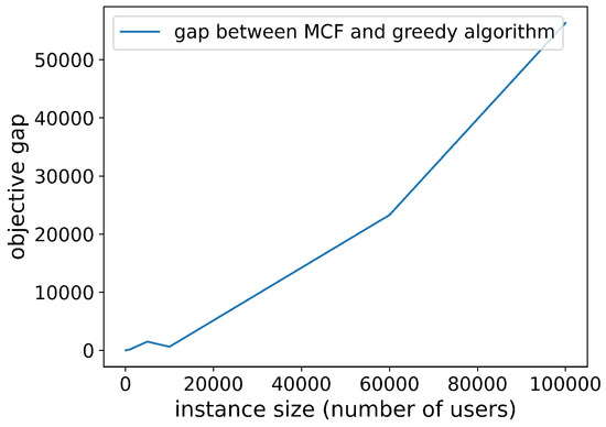
Figure 8.
Objective gap between greedy algorithm and minimum-cost flow.
In terms of computation time, the optimization process using Cplex to obtain the optimal solution is significantly greater than that of the minimum-cost flow algorithm, with the greedy algorithm demonstrating the fastest solving speed. Table 9 presents the solving speeds of these three optimization algorithms on instances of different sizes. For instance, the first row of Table 9 indicates that in instance 121400 with 100 users, the integer programming solved using Cplex requires 0.063 s, the min cost flow requires only 0.016 s, and the greedy algorithm requires 0.001 s. The disparity in solving time increases with the size of the instances.
Table 9.
Solving Time of three algorithms on different instances (in seconds) when .
Theoretically, the solving speed of the minimum cost flow problem is significantly faster than obtaining an exact solution in the integer linear programming problem. According to the analysis of the minimum cost flow formulation in Table 10, although the number of decision variables and constraints increases, the decision variables transition from being original 0–1 integers to real numbers.
Table 10.
Complexity Analysis of Integer Programming (IP) and Minimum Cost Flow (MCF).
5. Discussion
5.1. Key Findings
We conducted an experimental evaluation of various predictive models and optimization algorithms for user allocation tasks, aiming to maximize either the number of orders or the total sales revenue. Using a sliding window approach, we generated multiple instances of user behavior data, enabling us to frame the problem as a binary classification task for predicting purchase outcomes. We explored three predictive models—Logistic Regression, xgBoost, and Wide&Deep—in combination with different optimization strategies, including greedy algorithms and minimum-cost flow algorithms, to derive user allocation plans.
The experimental results demonstrate that the WDL model, leveraging its neural architecture’s capability for implicit feature interaction learning, exhibits robust stability in cross-border scenarios (e.g., seasonal product fluctuations) [56], with superior AUC performance compared to XGBoost and LR (WDL > XGBoost > LR). By combining wide and deep components, the WDL model captures both low-order explicit feature relationships through linear models and high-order feature interactions via deep learning [57], thereby enhancing overall performance. This finding aligns with Cheng et al.’s validation of the WDL model’s effectiveness in recommendation systems [47]. XGBoost demonstrates strong baseline performance by capturing complex nonlinear relationships through multiple decision trees and identifying key features to establish prediction rules. This confirms Grinsztajn’s proposition regarding XGBoost’s excellent performance on structured data [58,59]. The linear assumptions of LR result in significantly inferior performance across all metrics, especially in recall, exposing its fundamental constraints in complex behavioral modeling.
In the optimization problem of e-commerce promotion resource allocation, different algorithmic strategies demonstrate significantly distinct performance characteristics. The regional hot-sale strategy, based on historical sales data, is a heuristic method relying on statistical rules, whose performance is inherently constrained by historical data. The greedy algorithm, which prioritizes the current optimal product-user combinations for promotion, exhibits linear time complexity and achieves better results than the hot-sale approach. However, its myopic optimization nature based on local optimal choices prevents it from guaranteeing global optimality.
Regarding theoretical optimality, integer programming methods (e.g., branch and bound algorithms) can guarantee globally optimal solutions through systematic exploration of the entire solution space. However, as the problem is inherently NP-hard, its exponentially growing computational complexity with problem size severely limits practical applicability in large-scale e-commerce scenarios. The minimum cost flow method transforms the original problem into an equivalent network flow problem, which not only preserves the original optimization objectives but also maintains all critical business constraints through techniques like introducing virtual nodes and capacity constraints. While retaining optimality properties, it substantially reduces computational complexity. Leveraging the special structure of network flow problems, polynomial-time algorithms can be employed for efficient solving, achieving a balance between computational efficiency and solution quality.
The integration of predictive models with optimization algorithms yields significant improvements compared to regional best-selling strategies. Particularly, the combination of the WDL model with the minimum-cost flow algorithm achieves at least 10% increase in orders and approximately 20% growth in sales revenue across all instances. Furthermore, the minimum-cost flow algorithm outperforms the greedy algorithm in providing optimal solutions, especially as instance scales increase. To achieve optimal results, it is essential to prioritize the development of high-performing predictive models, as prediction inaccuracies can induce decision errors, which are quantified by Elmachtoub et al. [35].
5.2. Theoretical Implications
This study advances theoretical understanding in three key aspects. First, the proposed two-stage optimization framework systematically addresses critical limitations in constraint modeling by incorporating cross-category resource competition and user fatigue dynamics. The introduction of a decay hyperparameter quantitatively captures diminishing marginal effects of successive promotions, providing a principled approach to model user behavioral responses. Second, the reformulation of the original integer programming problem into an equivalent minimum-cost flow network ensures strict constraint compliance while achieving polynomial-time computational complexity, enabling scalable solutions for large-scale marketing allocation problems.
Third, empirical evidence from four experimental instances demonstrates the differential impacts of prediction and optimization components. Variations in prediction models account for approximately 35% performance differences, while optimization algorithms contribute up to 20% variation. This quantifies the critical role of prediction accuracy as an upper bound for optimization effectiveness, establishing a theoretical foundation for prediction-priority [60] frameworks in joint optimization tasks.
5.3. Practical Implications
This research provides an effective framework for the optimization of multi-product marketing promotion, which can significantly increase the number of orders and sales. We recommend prioritizing the improvement of the prediction model, which can bring about a more significant improvement. We have provided practical algorithm selection suggestions for different business scenarios. The greedy algorithm, due to its fast problem-solving ability, is suitable for large-scale problem scenarios with high real-time requirements but relatively low requirements for an optimal solution. Although integer programming has a high computational cost, it can provide the optimal solution and is convenient for handling complex constraints. It is suitable for scenarios where the quality of the solution is extremely high and the computational time is not the main limit. The minimum cost flow algorithm achieves a good balance between efficiency and solution quality. It is particularly suitable for large-scale network flow problems and can provide high-quality solutions within a reasonable time.
The model of this study has wide applicability and can be generalized to other fields of resource allocation. For example, in the internal audit plan [61], auditable units can be regarded as “customers” and audit resources as “marketing resources”, and our model can be utilized to optimize the allocation of audit tasks to minimize risks. It can also be extended to areas such as inventory distribution and the allocation of customer service resources.
5.4. Limitations and Future Work
First, the assumption of linear decay simplifies complex user responses and may underestimate nonlinear drops in engagement. Second, we do not model product interdependencies like complementarity and substitution effects, which might cause suboptimal allocations in related product categories. Third, the static optimization framework is not adaptable to real-time behavioral changes during promotional campaigns. For future research, we can develop dynamic joint optimization models with reinforcement learning to incorporate real-time feedback, such as cart additions [62]. Lastly, exploring end-to-end trainable architectures using differentiable optimization layers to reduce the discrepancy between prediction and optimization is a promising direction.
6. Conclusions
This study proposes a two-stage method to solve the multi-product marketing resource allocation in cross-border e-commerce, considering the user interest decay effect. Through comprehensive evaluations of various prediction models and optimization algorithms, we demonstrate that the WDL and XGBoost models can effectively support downstream optimization tasks. In the optimization stage, the problem was transformed into a minimum cost flow network model, achieving precise solutions with polynomial time complexity, thus making large-scale commercial deployment feasible. Experimental results show that our framework significantly outperforms baseline strategies and enhances marketing effectiveness.
Our findings offer practical insights for e-commerce platform deployment. Regarding algorithm selection, the minimum-cost flow method is preferred for large-scale problems requiring optimality guarantees, while greedy algorithms are suitable for scenarios where suboptimal solutions suffice. The study shows that the accuracy of prediction models significantly impacts optimization results. It is recommended to prioritize improving the accuracy of prediction models. Future research adopting end-to-end learning can establish a prediction-priority optimization framework to overcome the limitations of the current two-stage method.
Author Contributions
Y.X.: Conceptualization, Methodology, Writing, Visualization, Validation, Software. H.-Q.Y.: Funding acquisition, Writing. W.Z.: Conceptualization, Methodology, Software, Project administration. All authors have read and agreed to the published version of the manuscript.
Funding
This work was supported in part by the NSFC/RGC Joint Research Scheme under Grant No. N_PolyU590/22 (72261160393).
Institutional Review Board Statement
Not applicable.
Informed Consent Statement
Not applicable.
Data Availability Statement
Codes and Data are available from the corresponding author upon request.
Acknowledgments
The authors would like to sincerely thank the editor and reviewers for their kind comments.
Conflicts of Interest
The authors declare no conflicts of interest.
Appendix A
Appendix A.1. Pseudo-Code of Greedy Rule-Based Algorithm
The pseudo-code of the greedy rule-based algorithm is described in Algorithm A1.
| Algorithm A1: Promotion allocation based on greedy. |
|
Appendix A.2. Sup-Problem Example
We provide small examples for sub-problem 1 and sub-problem 2 to help illustrate the problem formulation.
Example of sub-problem 1: During the manager’s introduction of business requirements, we learned that when a customer receives multiple promotional activities in a short period, the effectiveness of the subsequent promotion tends to decrease. We define as calculated by a predictive model, and as the result of multiplying by a real number in the range of 0 to 1, denoted as the hyperparameter “decay”. Table A1 provides an example of sub-problem 1 when , , , ).
Table A1.
Example of sub-problem 1.
Table A1.
Example of sub-problem 1.
| Product | Customer Index | ||
|---|---|---|---|
| 1 | 1 | 0.385 | 0.385 × 0.9 |
| 1 | 5 | 0.375 | 0.375 × 0.9 |
| 1 | 3 | 0.166 | 0.166 × 0.9 |
| 1 | 4 | 0.109 | 0.109 × 0.9 |
| 1 | 2 | 0.237 | 0.237 × 0.9 |
| 2 | 5 | 0.401 | 0.401 × 0.9 |
| 2 | 1 | 0.103 | 0.103 × 0.9 |
| 2 | 4 | 0.206 | 0.206 × 0.9 |
| 2 | 2 | 0.012 | 0.012 × 0.9 |
| 2 | 3 | 0.190 | 0.190 × 0.9 |
Example of sub-problem 2: Table A2 presents an example for sub-problem 2 (when , , ), illustrating decision variables.
Table A2.
Example of sub-problem 2.
Table A2.
Example of sub-problem 2.
| Product | Customer | ||
|---|---|---|---|
| 1 | 1 | 1 | 0 |
| 1 | 5 | 0 | 1 |
| 1 | 3 | 0 | 0 |
| 1 | 4 | 0 | 0 |
| 1 | 2 | 0 | 0 |
| 2 | 5 | 1 | 0 |
| 2 | 1 | 0 | 0 |
| 2 | 4 | 0 | 1 |
| 2 | 2 | 0 | 0 |
| 2 | 3 | 0 | 0 |
Appendix A.3. Experiments on Other Instances
In the main body of the paper, we present detailed results for instance 1. Here we provide detailed results for the other three instances.
Table A3.
Results of instance 2 with optimization for the number of orders.
Table A3.
Results of instance 2 with optimization for the number of orders.
| Product | Hot-Selling | Greedy Algorithm | Minimum Cost Flow | ||||
|---|---|---|---|---|---|---|---|
| ID | Area | LR | xgBoost | WDL | LR | xgBoost | WDL |
| 1 | 685 | 1049 | 965 | 976 | 965 | 1049 | 917 |
| 2 | 56 | 985 | 1268 | 1268 | 985 | 1268 | 996 |
| 3 | 991 | 1654 | 1706 | 1706 | 1654 | 1706 | 1654 |
| 4 | 2661 | 2716 | 2707 | 2714 | 2707 | 2716 | 2588 |
| 5 | 952 | 1082 | 1057 | 1057 | 1082 | 1057 | 1082 |
| 6 | 75 | 1408 | 990 | 992 | 990 | 1408 | 1408 |
| 7 | 774 | 359 | 382 | 381 | 382 | 362 | 756 |
| 8 | 867 | 884 | 883 | 883 | 884 | 883 | 883 |
| 9 | 1572 | 1184 | 1366 | 1367 | 1366 | 1182 | 1386 |
| 10 | 47 | 781 | 766 | 768 | 766 | 781 | 821 |
| Total | 8680 | 12,102 | 12,090 | 12,112 | 12,465 | 12,103 | 12,491 |
| Increase % | 0.00% | 39.42% | 39.29% | 39.54% | 43.61% | 39.44% | 43.91% |
Table A4.
Results of instance 2 with sales revenue optimization.
Table A4.
Results of instance 2 with sales revenue optimization.
| Product | Hot-Selling | Greedy Algorithm | Minimum Cost Flow | ||||
|---|---|---|---|---|---|---|---|
| ID | Area | LR | xgBoost | WDL | LR | xgBoost | WDL |
| 1 | 16,433.1 | 22,310.7 | 23,006.4 | 21,830.9 | 22,430.7 | 23,174.3 | 21,950.9 |
| 2 | 1377.6 | 24,673.8 | 27,675.0 | 26,617.2 | 24,698.4 | 27,699.6 | 26,617.2 |
| 3 | 42,603.1 | 73,641.9 | 73,598.9 | 70,847.5 | 73,899.8 | 73,856.8 | 71,062.5 |
| 4 | 58,515.4 | 59,592.9 | 55,744.7 | 56,756.2 | 59,724.8 | 55,854.6 | 56,888.1 |
| 5 | 34,262.5 | 36,493.9 | 36,493.9 | 38,833.2 | 36,529.9 | 36,529.9 | 38,941.2 |
| 6 | 4208.3 | 79,002.9 | 79,002.9 | 79,002.9 | 79,002.9 | 79,002.9 | 79,002.9 |
| 7 | 123,066.0 | 57,717.0 | 60,738.0 | 119,886.0 | 57,558.0 | 60,579.0 | 119,409.0 |
| 8 | 251,421.3 | 25,6641.2 | 256,641.2 | 256,641.2 | 256,641.2 | 256,641.2 | 256,641.2 |
| 9 | 39,284.3 | 33,211.7 | 33,686.5 | 34,611.2 | 33,236.7 | 33,711.5 | 34,711.1 |
| 10 | 751.5 | 11,448.8 | 11,416.9 | 11,384.9 | 11,480.8 | 11,480.8 | 11,416.9 |
| Total | 571,923.1 | 654,734.7 | 658,004.2 | 716,411.1 | 655,203.1 | 658,530.6 | 716,640.8 |
| Increase % | 0.00% | 14.48% | 15.05% | 25.26% | 14.56% | 15.14% | 25.30% |
Table A5.
Results of instance 3 with optimization for the number of orders.
Table A5.
Results of instance 3 with optimization for the number of orders.
| Product | Hot-Selling | Greedy Algorithm | Minimum Cost Flow | ||||
|---|---|---|---|---|---|---|---|
| ID | Area | LR | xgBoost | WDL | LR | xgBoost | WDL |
| 1 | 825 | 1314 | 499 | 1314 | 1314 | 501 | 1314 |
| 2 | 803 | 1113 | 1023 | 1333 | 1114 | 975 | 1333 |
| 3 | 768 | 157 | 1257 | 458 | 157 | 1257 | 458 |
| 4 | 1132 | 1801 | 1908 | 928 | 1801 | 1910 | 928 |
| 5 | 736 | 830 | 976 | 989 | 926 | 1080 | 1091 |
| 6 | 1007 | 747 | 777 | 754 | 747 | 777 | 754 |
| 7 | 1129 | 1862 | 1545 | 1857 | 1862 | 1554 | 1857 |
| 8 | 772 | 1279 | 1268 | 1279 | 1279 | 1268 | 1279 |
| 9 | 786 | 650 | 1273 | 1099 | 650 | 1283 | 1099 |
| 10 | 1184 | 73 | 1740 | 94 | 73 | 1753 | 94 |
| Total | 9142 | 9826 | 12,266 | 10,105 | 9923 | 12,358 | 10,207 |
| Increase % | 0.00% | 7.48% | 34.17% | 10.53% | 8.54% | 35.18% | 11.65% |
Table A6.
Results of instance 3 with sales revenue optimization.
Table A6.
Results of instance 3 with sales revenue optimization.
| Product | Hot-Selling | Greedy Algorithm | Minimum Cost Flow | ||||
|---|---|---|---|---|---|---|---|
| ID | Area | LR | xgBoost | WDL | LR | xgBoost | WDL |
| 1 | 43,716.8 | 69,628.9 | 26,177.1 | 69,522.9 | 69,628.9 | 26,071.1 | 69,628.9 |
| 2 | 49,778.0 | 66,205.3 | 81,454.9 | 81,826.8 | 65,957.4 | 81,516.9 | 81,826.8 |
| 3 | 46,072.3 | 2039.7 | 75,347.4 | 22,496.3 | 1499.8 | 75,407.4 | 18,536.9 |
| 4 | 305,628.7 | 516,760.9 | 516,760.9 | 516,490.9 | 516,760.9 | 516,760.9 | 516,220.9 |
| 5 | 220,064.0 | 256,542.0 | 299,000.0 | 299,299.0 | 285,844.0 | 328,900.0 | 316,641.0 |
| 6 | 51,346.9 | 2906.4 | 38,140.5 | 30,594.0 | 2906.4 | 37,987.6 | 30,339.1 |
| 7 | 60,954.7 | 100,367.4 | 50,102.7 | 100,097.5 | 100,205.4 | 47,943.1 | 100,043.5 |
| 8 | 122,748.0 | 203,361.0 | 202,566.0 | 2,025,663.0 | 1279.0 | 203,361.0 | 203,361.0 |
| 9 | 25,930.1 | 132.0 | 2804.2 | 0.0 | 132.0 | 1121.7 | 0.0 |
| 10 | 54,452.2 | 92.0 | 32,514.9 | 0.0 | 92.0 | 29,433.6 | 0.0 |
| Total | 980,691.7 | 1,218,035.5 | 1,324,868.5 | 1,322,893.3 | 1,246,387.6 | 1,348,503.2 | 1,336,598.0 |
| Increase % | 0.00% | 24.20% | 35.10% | 34.89% | 27.09% | 37.51% | 36.29% |
Table A7.
Results of instance 4 with optimization for the number of orders.
Table A7.
Results of instance 4 with optimization for the number of orders.
| Product | Hot-Selling | Greedy Algorithm | Minimum Cost Flow | ||||
|---|---|---|---|---|---|---|---|
| ID | Area | LR | xgBoost | WDL | LR | xgBoost | WDL |
| 1 | 378 | 67 | 326 | 1287 | 67 | 326 | 1286 |
| 2 | 107 | 71 | 195 | 1012 | 71 | 195 | 371 |
| 3 | 369 | 105 | 194 | 690 | 97 | 194 | 561 |
| 4 | 1208 | 983 | 972 | 1139 | 983 | 972 | 1138 |
| 5 | 1562 | 1342 | 1441 | 1425 | 1342 | 1441 | 2462 |
| 6 | 330 | 624 | 580 | 281 | 678 | 649 | 281 |
| 7 | 343 | 271 | 908 | 308 | 271 | 908 | 308 |
| 8 | 387 | 819 | 71 | 366 | 835 | 71 | 380 |
| 9 | 431 | 46 | 442 | 414 | 46 | 442 | 587 |
| 10 | 162 | 897 | 158 | 233 | 904 | 158 | 831 |
| Total | 5277 | 5225 | 5287 | 7155 | 5294 | 5356 | 8205 |
| Increase % | 0.00% | −0.99% | 0.19% | 35.59% | 0.32% | 1.50% | 55.49% |
Table A8.
Results of instance 4 with sales revenue optimization.
Table A8.
Results of instance 4 with sales revenue optimization.
| Product | Hot-Selling | Greedy Algorithm | Minimum Cost Flow | ||||
|---|---|---|---|---|---|---|---|
| ID | Area | LR | xgBoost | WDL | LR | xgBoost | WDL |
| 1 | 5507.5 | 218.6 | 0.0 | 0.0 | 218.6 | 0.0 | 0.0 |
| 2 | 4486.5 | 2725.5 | 3857.6 | 2473.9 | 2641.6 | 3857.6 | 2473.9 |
| 3 | 15,125.3 | 3320.2 | 1680.6 | 655.8 | 3279.2 | 1680.6 | 573.9 |
| 4 | 326,147.9 | 491,651.8 | 492,461.8 | 492,191.8 | 496,511.6 | 505,421.3 | 505,691.3 |
| 5 | 467,038.0 | 760,058.0 | 760,955.0 | 758,563.0 | 760,058.0 | 762,450.0 | 762,749.0 |
| 6 | 131,670.0 | 248,976.0 | 234,213.0 | 243,789.0 | 260,946.0 | 256,557.0 | 248,577.0 |
| 7 | 119,707.0 | 314,100.0 | 317,241.0 | 317,241.0 | 317,241.0 | 317,241.0 | 317,241.0 |
| 8 | 13,928.1 | 2843.2 | 144.0 | 0.0 | 2807.2 | 144.0 | 0.0 |
| 9 | 25,855.7 | 5879.0 | 71,388.1 | 84,345.9 | 5759.0 | 68,208.6 | 84,465.9 |
| 10 | 4534.4 | 783.7 | 0.0 | 0.0 | 783.7 | 0.0 | 0.0 |
| Total | 1,114,000.4 | 1,830,555.9 | 1,881,941.0 | 1,899,260.4 | 1,850,245.9 | 1,915,560.0 | 1,921,771.9 |
| Increase % | 0.00% | 59.20% | 63.67% | 65.18% | 60.91% | 66.59% | 67.13% |
References
- Bolos, C.; Idemudia, E.C.; Mai, P.; Rasinghani, M.; Smith, S. Conceptual models on the effectiveness of e-marketing strategies in engaging consumers. J. Int. Technol. Inf. Manag. 2016, 25, 3. [Google Scholar] [CrossRef]
- Kundu, N.; Mustafa, F.; Chola, C. Artificial intelligence in retail marketing. In Artificial Intelligence for Business; Productivity Press: New York, NY, USA, 2023; pp. 86–107. [Google Scholar]
- Maria, V.; Aziz, A.F.; Rahmawati, D. Meningkatkan daya saing UMKM lokal melalui strategi pemasaran digital di era digital. OPTIMAL J. Ekon. Dan Manaj. 2024, 4, 208–220. [Google Scholar] [CrossRef]
- Thomas, M.; Goic, M.; Kalyanam, K. Long Lags and Large Returns: Experimental Evidence from Advertising to Businesses. Manag. Sci. 2025. [Google Scholar] [CrossRef]
- Chaparro-Peláez, J.; Hernández-García, Á.; Lorente-Páramo, Á.-J. May I have your attention, please? An investigation on opening effectiveness in e-mail marketing. Rev. Manag. Sci. 2022, 16, 2261–2284. [Google Scholar] [CrossRef]
- Merisavo, M.; Raulas, M. The impact of e-mail marketing on brand loyalty. J. Prod. Brand Manag. 2004, 13, 498–505. [Google Scholar] [CrossRef]
- Gummesson, E. Total Relationship Marketing; Routledge: Oxfordshire, UK, 2011. [Google Scholar]
- Debnath, A.; Hossan, M.Z.; Sharmin, S.; Hosain, M.S.; Johora, F.T.; Hossain, M. Analyzing and Forecasting of Real-Time Marketing Campaign Performance and ROI in the US Market. In Proceedings of the 2024 International Conference on Intelligent Cybernetics Technology & Applications (ICICyTA), Bali, Indonesia, 17–19 December 2024; pp. 332–337. [Google Scholar]
- Li, X.; Yu, H.; Sun, C. Direct Mail or Bonded Warehouse? Logistics Mode Selection in Cross-Border E-Commerce under Exchange Rate Risk. J. Theor. Appl. Electron. Commer. Res. 2024, 19, 2312–2342. [Google Scholar] [CrossRef]
- Deng, G.; Zhang, J.; Xu, Y. How e-commerce platforms build channel power: The role of AI resources and market-based assets. J. Bus. Ind. Mark. 2024, 39, 173–188. [Google Scholar] [CrossRef]
- Gavilan, D.; Martinez-Navarro, G. Exploring user’s experience of push notifications: A grounded theory approach. Qual. Mark. Res. Int. J. 2022, 25, 233–255. [Google Scholar] [CrossRef]
- He, X.; Liu, Q.; Jung, S. The impact of recommendation system on user satisfaction: A moderated mediation approach. J. Theor. Appl. Electron. Commer. Res. 2024, 19, 448–466. [Google Scholar] [CrossRef]
- Chen, N.; Hu, M. Frontiers in service science: Data-driven revenue management: The interplay of data, model, and decisions. Serv. Sci. 2023, 15, 79–91. [Google Scholar] [CrossRef]
- Miao, X.; Li, Z.; Yan, Y.; Xu, A. A Tripartite Evolutionary Game-Based Cooperation Model of Cross-Border E-Commerce Logistics Alliances: A Case Study of China. J. Theor. Appl. Electron. Commer. Res. 2025, 20, 37. [Google Scholar] [CrossRef]
- Kellerer, H.; Pferschy, U.; Pisinger, D. The multiple-choice knapsack problem. In Knapsack Problems; Springer: Berlin/Heidelberg, Germany, 2004; pp. 317–347. [Google Scholar]
- Lopez, S. Optimizing marketing ROI with predictive analytics: Harnessing big data and AI for data-driven decision making. J. Artif. Intell. Res. 2023, 3, 9–36. [Google Scholar]
- Alves Gomes, M.; Meisen, T. A review on customer segmentation methods for personalized customer targeting in e-commerce use cases. Inf. Syst. Bus. Manag. 2023, 21, 527–570. [Google Scholar] [CrossRef]
- Zhang, S.; Liao, P.; Ye, H.Q.; Zhou, Z. Dynamic marketing resource allocation with two-stage decisions. J. Theor. Appl. Electron. Commer. Res. 2022, 17, 327–344. [Google Scholar] [CrossRef]
- Fu, M.; Chen, Q.; Lin, W.; Wang, P.; Zhang, W. Constructing a scene-based knowledge system for E-commerce industries: Business analysis and challenges. Data Intell. 2019, 1, 224–237. [Google Scholar] [CrossRef]
- Chen, Y.L.; Kuo, M.H.; Wu, S.Y.; Tang, K. Discovering recency, frequency, and monetary (RFM) sequential patterns from customers’ purchasing data. Electron. Commer. Res. Appl. 2009, 8, 241–251. [Google Scholar] [CrossRef]
- Saura, J.R.; Palacios-Marqués, D.; Ribeiro-Soriano, D. Digital marketing in SMEs via data-driven strategies: Reviewing the current state of research. J. Small Bus. Manag. 2023, 61, 1278–1313. [Google Scholar] [CrossRef]
- Linden, G.; Smith, B.; York, J. Amazon. com recommendations: Item-to-item collaborative filtering. IEEE Internet Comput. 2003, 7, 76–80. [Google Scholar] [CrossRef]
- deWet, S.; Ou, J. Finding users who act alike: Transfer learning for expanding advertiser audiences. In Proceedings of the 25th ACM SIGKDD International Conference on Knowledge Discovery & Data Mining, Anchorage, AK, USA, 4–8 August 2019; pp. 2251–2259. [Google Scholar]
- Ma, Q.; Wen, M.; Xia, Z.; Chen, D. A sub-linear, massive-scale look-alike audience extension system a massive-scale look-alike audience extension. In Proceedings of the Workshop on Big Data, Streams and Heterogeneous Source Mining: Algorithms, Systems, Programming Models and Applications, PMLR, San Francisco, CA, USA, 14 August 2016; pp. 51–67. [Google Scholar]
- Gao, Y.; Gupta, V.; Yan, J.; Shi, C.; Tao, Z.; Xiao, P.; Wang, C.; Yu, S.; Rosales, R.; Muralidharan, A.; et al. Near real-time optimization of activity-based notifications. In Proceedings of the 24th ACM SIGKDD International Conference on Knowledge Discovery & Data Mining, London, UK, 19–23 August 2018; pp. 283–292. [Google Scholar]
- Iqbal, S.T.; Bailey, B.P. Oasis: A framework for linking notification delivery to the perceptual structure of goal-directed tasks. ACM Trans. Comput. Hum. Interact. (TOCHI) 2010, 17, 1–28. [Google Scholar] [CrossRef]
- Zhou, H.; Li, S.; Jiang, G.; Zheng, J.; Wang, D. Direct heterogeneous causal learning for resource allocation problems in marketing. In Proceedings of the AAAI Conference on Artificial Intelligence, Montreal, QC, Canada, 8–10 August 2023; Volume 37, pp. 5446–5454. [Google Scholar]
- Yuan, J.; Mensah-Boateng, T.; Tang, S. Influencer Marketing Augmented Personalized Assortment Planning: A Two-stage Optimization Problem. In Proceedings of the International AAAI Conference on Web and Social Media, Buffalo, NY, USA, 3–6 June 2024; Volume 18, pp. 1753–1765. [Google Scholar]
- Lu, H.; Simester, D.; Zhu, Y. Optimizing scalable targeted marketing policies with constraints. Mark. Sci. 2025. [Google Scholar] [CrossRef]
- Albert, J.; Goldenberg, D. E-commerce promotions personalization via online multiple-choice knapsack with uplift modeling. In Proceedings of the 31st ACM International Conference on Information & Knowledge Management, Atlanta, GA, USA, 17–21 October 2022; pp. 2863–2872. [Google Scholar]
- Baardman, L.; Boroujeni, S.B.; Cohen-Hillel, T.; Panchamgam, K.; Perakis, G. Detecting customer trends for optimal promotion targeting. Manuf. Serv. Oper. Manag. 2023, 25, 448–467. [Google Scholar] [CrossRef]
- Wang, C.; Shi, X.; Xu, S.; Wang, Z.; Fan, Z.; Feng, Y.; You, A.; Chen, Y. A Multi-stage Framework for Online Bonus Allocation Based on Constrained User Intent Detection. In Proceedings of the 29th ACM SIGKDD Conference on Knowledge Discovery and Data Mining, Long Beach, CA, USA, 6–10 August 2023; pp. 5028–5038. [Google Scholar]
- Liu, Y.; Zhou, C.; Zhang, P.; Pan, S.; Li, Z.; Chen, H. Decision-focused Graph Neural Networks for Combinatorial Optimization. arXiv 2024, arXiv:2406.03647. [Google Scholar]
- Nguyen, D.M.; Diep, N.T.; Nguyen, T.Q.; Le, H.B.; Nguyen, T.; Nguyen, T.; Nguyen, T.; Ho, N.; Xie, P.; Wattenhofer, R.; et al. Logra-med: Long context multi-graph alignment for medical vision-language model. arXiv 2024, arXiv:2410.02615. [Google Scholar]
- Elmachtoub, A.N.; Grigas, P. Smart “predict, then optimize”. Manag. Sci. 2022, 68, 9–26. [Google Scholar] [CrossRef]
- Zhou, H.; Huang, R.; Li, S.; Jiang, G.; Zheng, J.; Cheng, B.; Lin, W. Decision focused causal learning for direct counterfactual marketing optimization. In Proceedings of the 30th ACM SIGKDD Conference on Knowledge Discovery and Data Mining, Barcelona, Spain, 25–29 August 2024; pp. 6368–6379. [Google Scholar]
- Yan, Z.; Wang, S.; Zhou, G.; Lin, J.; Jiang, P. An end-to-end framework for marketing effectiveness optimization under budget constraint. arXiv 2023, arXiv:2302.04477. [Google Scholar]
- Harris, L.C.; Ogbonna, E. The organization of marketing: A study of decentralized, devolved and dispersed marketing activity. J. Manag. Stud. 2003, 40, 483–512. [Google Scholar] [CrossRef]
- Anand, R.; Aggarwal, D.; Kumar, V. A comparative analysis of optimization solvers. J. Stat. Manag. Syst. 2017, 20, 623–635. [Google Scholar] [CrossRef]
- Kovács, P. Minimum-cost flow algorithms: An experimental evaluation. Optim. Methods Softw. 2015, 30, 94–127. [Google Scholar] [CrossRef]
- Guercini, S.; Freeman, S.M. How international marketers make decisions: Exploring approaches to learning and using heuristics. Int. Mark. Rev. 2023, 40, 429–451. [Google Scholar] [CrossRef]
- Deldjoo, Y.; Nazary, F.; Ramisa, A.; Mcauley, J.; Pellegrini, G.; Bellogin, A.; Noia, T.D. A review of modern fashion recommender systems. ACM Comput. Surv. 2023, 56, 1–37. [Google Scholar] [CrossRef]
- Zhang, X.; Kumar, V.; Cosguner, K. Dynamically managing a profitable email marketing program. J. Mark. Res. 2017, 54, 851–866. [Google Scholar] [CrossRef]
- Kahneman, D.; Tversky, A. Prospect theory: An analysis of decision under risk. In Handbook of the Fundamentals of Financial Decision Making: Part I; World Scientific: Singapore, 2013; pp. 99–127. [Google Scholar]
- Wright, R. Logistic regression. In Reading and Understanding Multivariate Statistics; American Psychological Association: Washington, DC, USA, 1995. [Google Scholar]
- Ester, M.; Kriegel, H.; Xu, X. XGBoost: A scalable tree boosting system. In Proceedings of the 22Nd ACM SIGKDD International Conference on Knowledge Discovery and Data Mining, San Francisco, CA, USA, 13–17 August 2016; p. 785. [Google Scholar]
- Cheng, H.T.; Koc, L.; Harmsen, J.; Shaked, T.; Chandra, T.; Aradhye, H.; Anderson, G.; Corrado, G.; Chai, W.; Ispir, M.; et al. Wide & deep learning for recommender systems. In Proceedings of the 1st Workshop on Deep Learning for Recommender Systems, Boston, MA, USA, 15 September 2016; pp. 7–10. [Google Scholar]
- Shen, W. DeepCTR: Easy-to-Use, Modular and Extendible Package of Deep-Learning Based CTR Models. 2017. Available online: https://github.com/shenweichen/deepctr (accessed on 15 January 2025).
- Zeybek, Ö.; Ülengin, B. The effect of sales promotions intensity on volume and variability in category sales of large retailers. J. Mark. Anal. 2022, 1–11. [Google Scholar] [CrossRef]
- Ahuja, R.K.; Magnanti, T.L.; Orlin, J.B. Network Flows: Theory, Algorithms, and Applications; Prentice Hall: Englewood Cliffs, NJ, USA, 1993. [Google Scholar]
- Edmonds, J.; Karp, R.M. Theoretical improvements in algorithmic efficiency for network flow problems. J. ACM (JACM) 1972, 19, 248–264. [Google Scholar] [CrossRef]
- Karp, R.M. Reducibility among combinatorial problems. In 50 Years of Integer Programming 1958–2008: From the Early Years to the State-of-the-Art; Springer: Berlin/Heidelberg, Germany, 2009; pp. 219–241. [Google Scholar]
- Moore, E.F. The shortest path through a maze. In Proceedings of the International Symposium on the Theory of Switching, Cambridge, UK, 2–5 April 1959; Harvard University Press: London, UK, 1959; pp. 285–292. [Google Scholar]
- Goldberg, A.V.; Tarjan, R.E. Solving minimum-cost flow problems by successive approximation. In Proceedings of the Nineteenth Annual ACM Symposium on Theory of Computing, New York, NY, USA, 1 January 1987; pp. 7–18. [Google Scholar]
- Ford, L.R., Jr.; Fulkerson, D.R. A suggested computation for maximal multi-commodity network flows. Manag. Sci. 2004, 50, 1778–1780. [Google Scholar] [CrossRef]
- Simester, D.; Timoshenko, A.; Zoumpoulis, S.I. Targeting prospective customers: Robustness of machine-learning methods to typical data challenges. Manag. Sci. 2020, 66, 2495–2522. [Google Scholar] [CrossRef]
- Lin, H.; Ji, H. Improved Wide&Deep Recommendation Algorithm for User Behavioural Characteristics. In Proceedings of the 13th International Conference of Information and Communication Technology (ICTech), Xiamen, China, 12–14 April 2024; pp. 234–238. [Google Scholar]
- Grinsztajn, L.; Oyallon, E.; Varoquaux, G. Why do tree-based models still outperform deep learning on typical tabular data? In Proceedings of the NIPS’22: 36th International Conference on Neural Information Processing Systems, New Orleans, LA, USA, 28 November–9 December 2022; Volume 35, pp. 507–520. [Google Scholar]
- Wu, J.; Li, Y.; Ma, Y. Comparison of XGBoost and the neural network model on the class-balanced datasets. In Proceedings of the IEEE 3rd International Conference on Frontiers Technology of Information and Computer (ICFTIC), Greenville, AC, USA, 12–14 November 2021; pp. 457–461. [Google Scholar]
- Kotary, J.; Fioretto, F.; Van Hentenryck, P.; Wilder, B. End-to-end constrained optimization learning: A survey. arXiv 2021, arXiv:2103.16378. [Google Scholar]
- Wang, X.; Ferreira, F.A.F.; Yan, P. A multi-objective optimization approach for integrated risk-based internal audit planning. Ann. Oper. Res. 2025, 346, 1811–1840. [Google Scholar] [CrossRef]
- Esmeli, R.; Gokce, A. An Analysis of Consumer Purchase Behavior Following Cart Addition in E-Commerce Utilizing Explainable Artificial Intelligence. J. Theor. Appl. Electron. Commer. Res. 2025, 20, 28. [Google Scholar] [CrossRef]

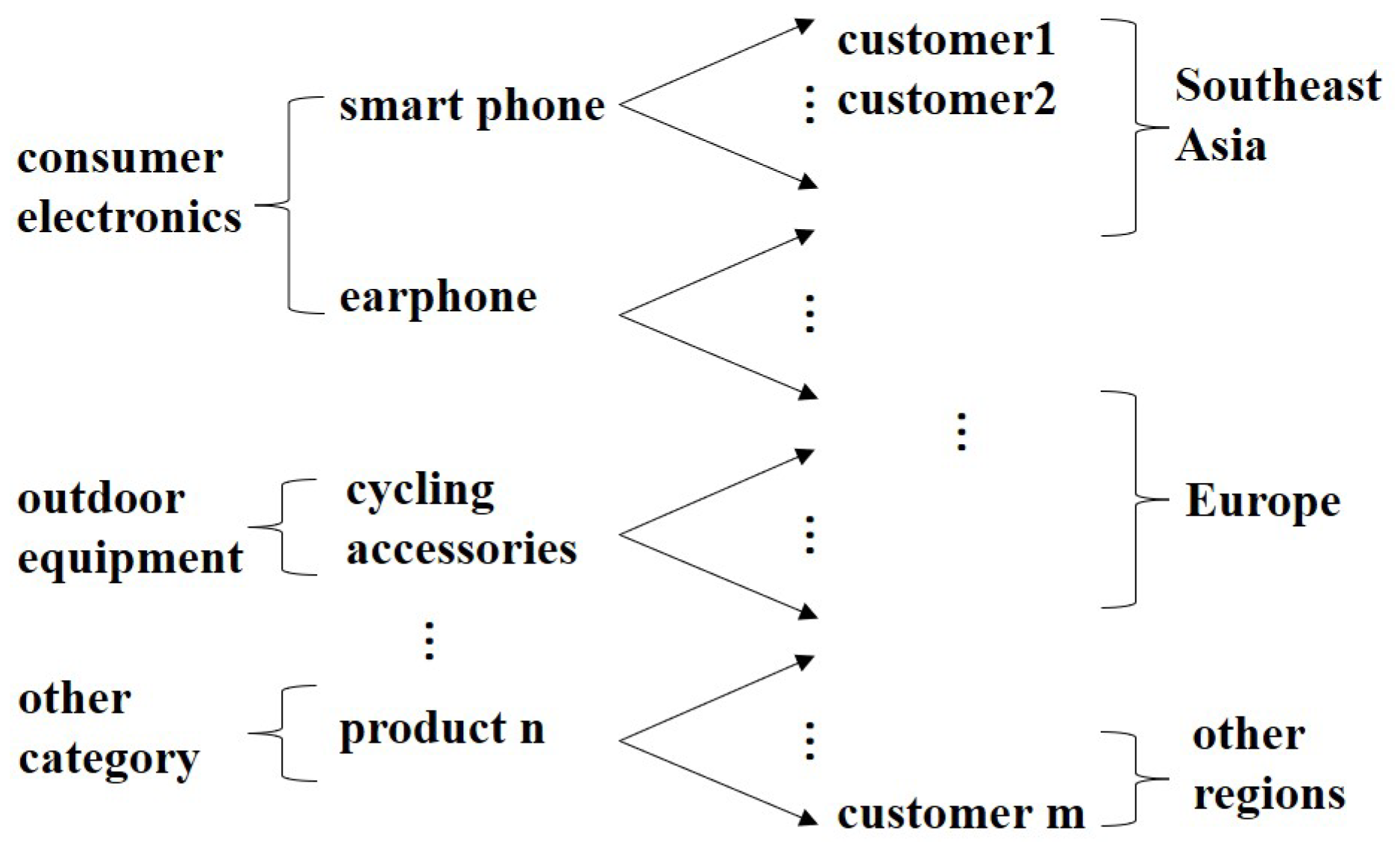
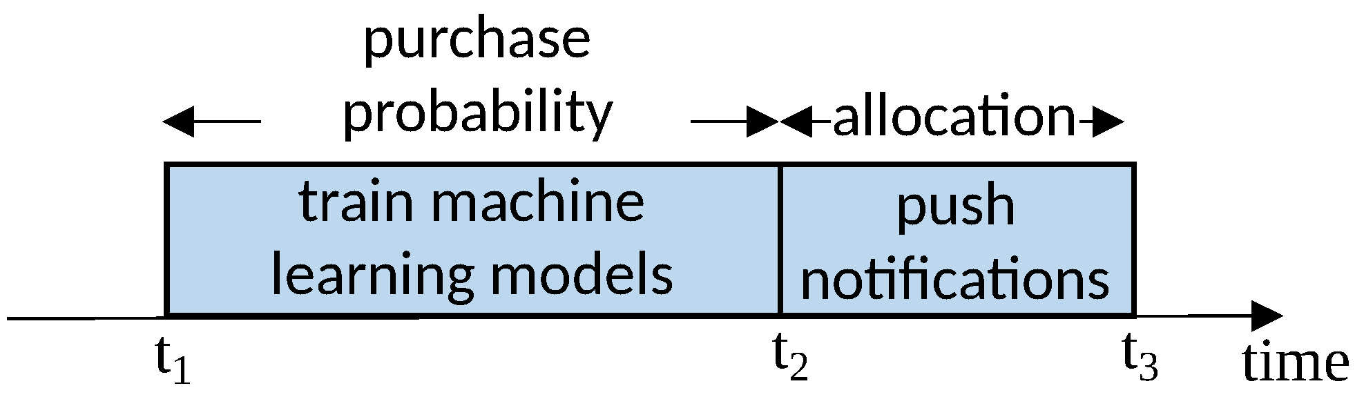

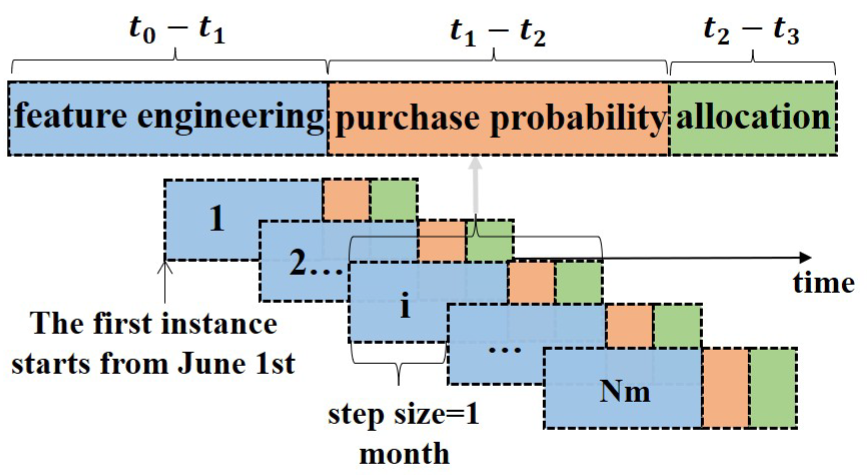
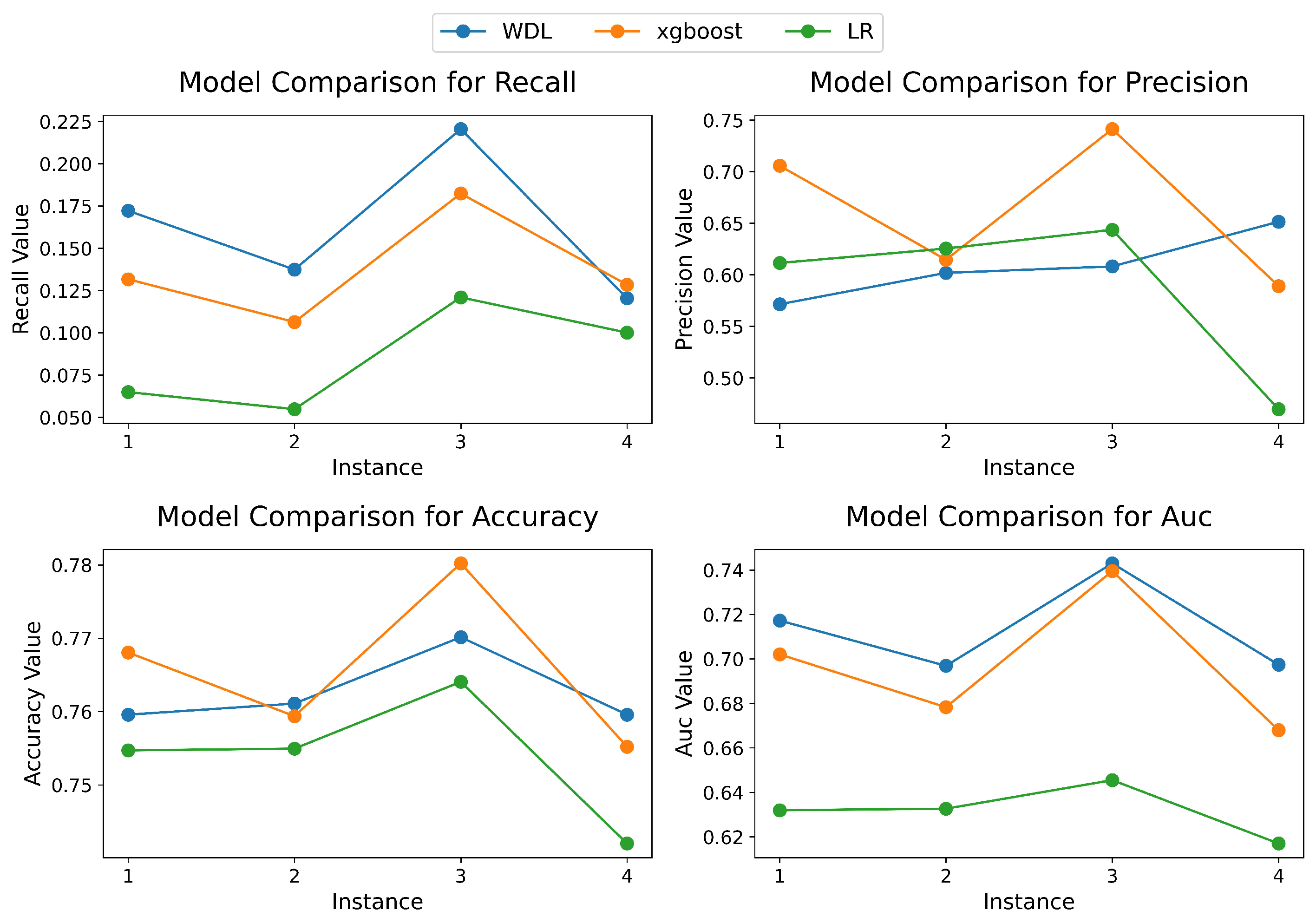
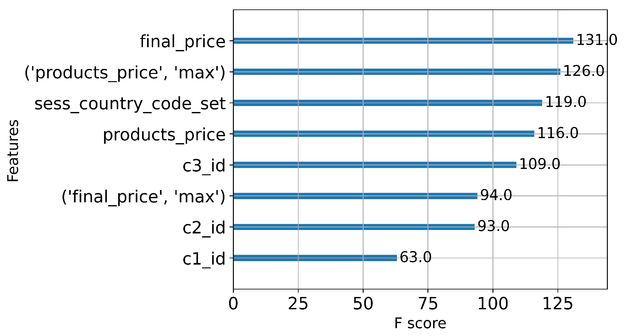

Disclaimer/Publisher’s Note: The statements, opinions and data contained in all publications are solely those of the individual author(s) and contributor(s) and not of MDPI and/or the editor(s). MDPI and/or the editor(s) disclaim responsibility for any injury to people or property resulting from any ideas, methods, instructions or products referred to in the content. |
© 2025 by the authors. Licensee MDPI, Basel, Switzerland. This article is an open access article distributed under the terms and conditions of the Creative Commons Attribution (CC BY) license (https://creativecommons.org/licenses/by/4.0/).