
Real-Time Detection and Quantification of Rail Surface Cracks Using Surface Acoustic Waves and Piezoelectric Patch Transducers

 , , , , ,
Abstract
1. Introduction
2. Materials and Methods
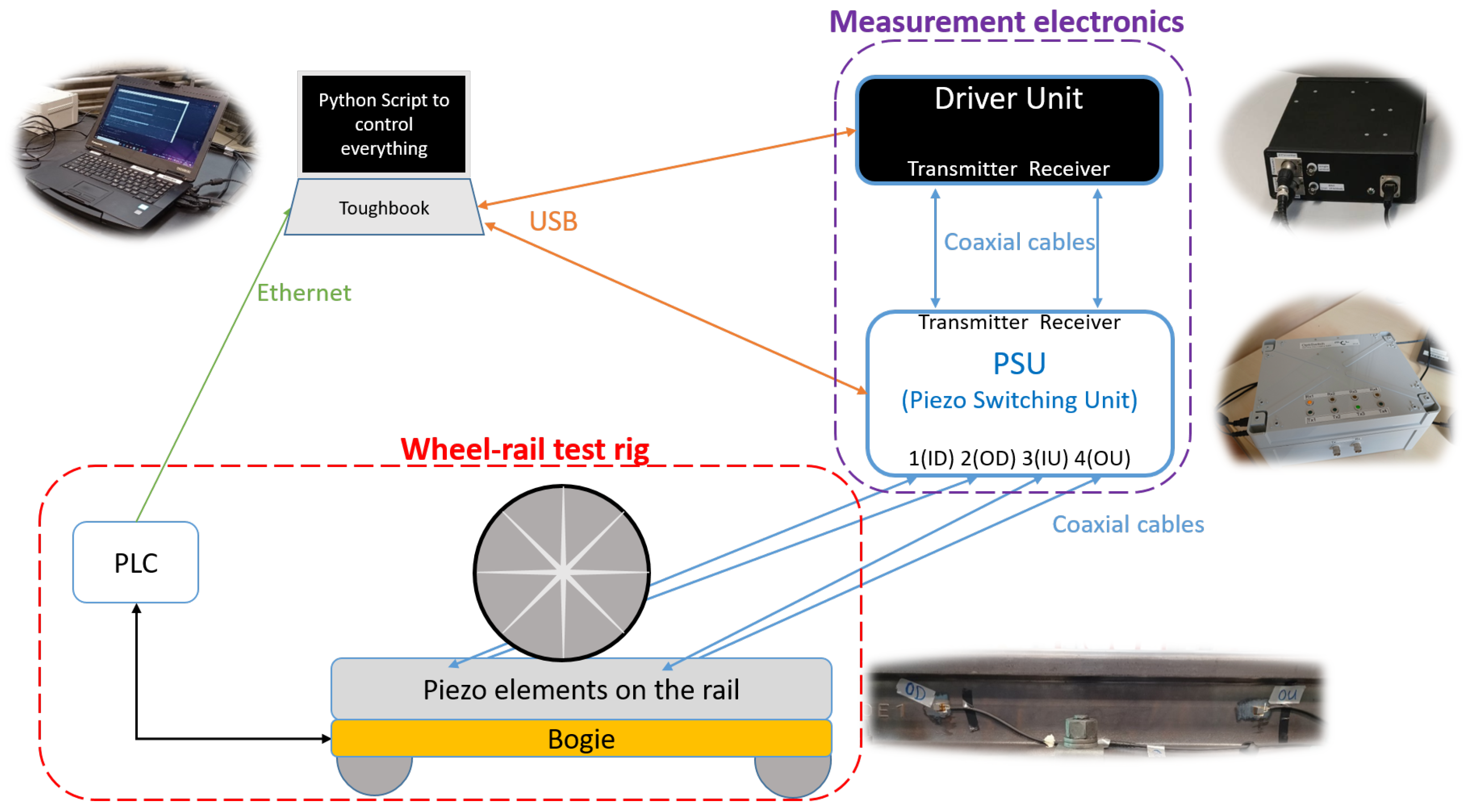
2.1. System Design
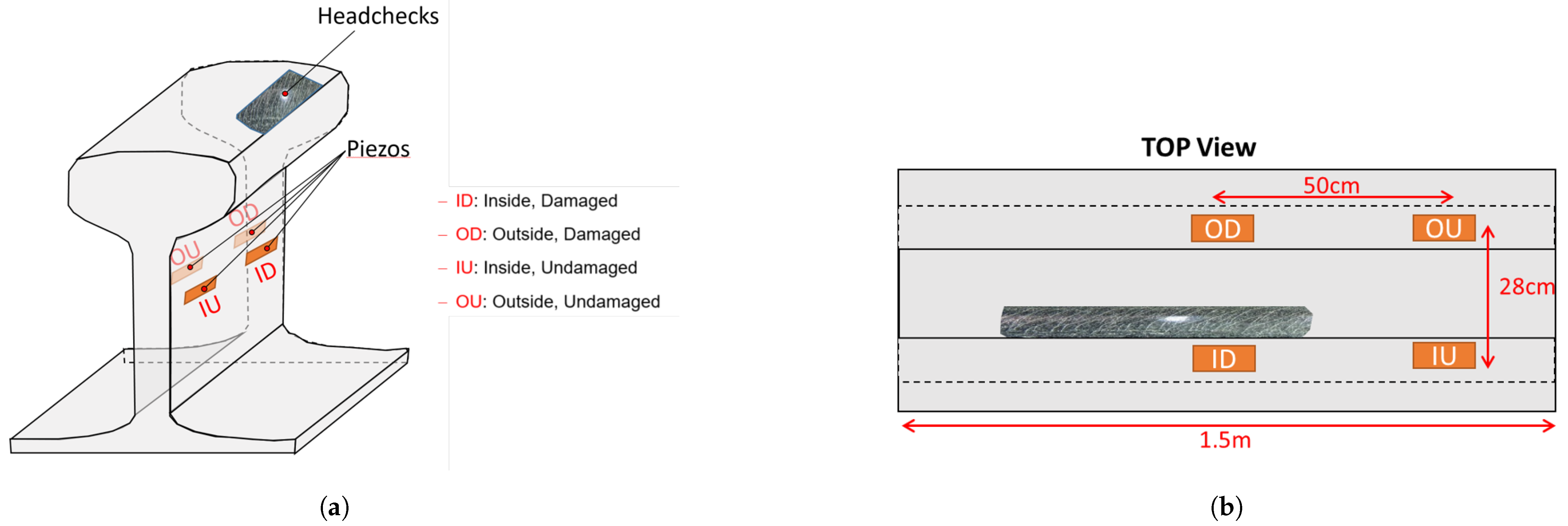
2.1.1. Transducers
2.1.2. Sender/Receiver Unit
2.2. Signal Processing Pipeline
- Noise reduction through cross-correlation.
- Identification of arrival time intervals.
- Estimation of damage index (DI) or crack depth by calculating transmission coefficients.
2.2.1. Deviation-Based Signal Processing Pipeline
- Interval detection:The received signal often exhibits a complex structure, containing noise, interference, and a combination of SAW and bulk waves. A typical received signal is shown in Figure 6. As seen, the signal has a weak amplitude and is influenced by various sources of noise and interference. To isolate the SAW component, a time-of-flight (ToF) analysis is conducted to estimate its expected arrival interval. In this case, a Rayleigh wave velocity of approximately 3000 m/s in steel is assumed, based on the material’s Young’s modulus and Poisson’s ratio. Given a transmitter–receiver spacing of 28 cm, the estimated time of flight is around 93 μs. Accordingly, a time window centered around this value—i.e., 93 μs ± (signal width/2)—is selected to accommodate uncertainties and ensure sufficient signal content for subsequent analysis, such as cross-correlation.This interval is visually marked and magnified in Figure 6 for clarity. It may be observed that a wave packet appears to arrive at nearly zero microseconds, which is not physically realistic. This early signal, also highlighted in the figure, is attributed to electromagnetic interference (EMI) between the sender and receiver ports, occurring at the moment the excitation signal is applied to the sender. The presence of such EMI is also indicated in the measurement results shown in [30] and further acknowledged in [31]. It is important to note that no additional excitation is applied to the sender port during the remaining signal duration, so no further EMI is expected. Although other wave modes, such as bulk waves, may be present in the time window following the EMI, the actual surface acoustic wave (SAW) packet arrives within the expected TOF window. Therefore, the EMI can be excluded, and the signal processing focuses only on the valid TOF interval.
- Calibration:Signal amplitudes can vary between cycles due to factors unrelated to crack development, such as adhesive aging or temperature fluctuations. To mitigate these effects, the algorithm calibrates the SAW signals using parts of the signal that remain unaffected by crack depth.
- Deviation calculation:Even within the expected SAW interval, the signal may contain bulk waves, electronic noise, and harmonics. These components often exhibit consistent patterns across cycles. By taking a snapshot of the signal at cycle zero, the algorithm calculates deviations for each subsequent cycle, effectively canceling out the unwanted components. The remaining deviation signal, in contrast, will primarily contain information related to crack depth evolution.
- Correlation:Despite previous preprocessing, the signal may still contain unwanted harmonics and noise at frequencies other than the excitation frequency. By correlating the processed signal with the transmitted signal, the algorithm acts as a matched filter, isolating the main frequency component for further analysis.
- Energy calculation:While many studies focus on peak amplitude, this approach considers the broader effect of the signal over a time interval. This is particularly important when using piezoelectric transducers, whose dimensions are comparable to the wavelength of the excitation, and excitation via burst signals extending over finite time. Instead of focusing on a single time point, the algorithm calculates the root mean square (RMS) value over the period of time the SAW takes to travel across the sensor, which correlates directly with crack depth.
- Normalization:The final output is an absolute value that becomes meaningful only when compared to a baseline measure. To achieve this, the calculated value is normalized with respect to the corresponding value at cycle zero (damage-free status).
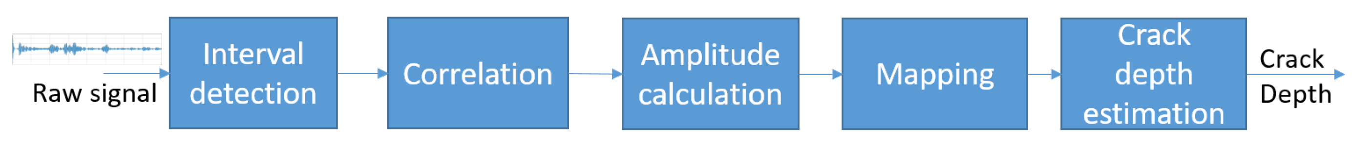
2.2.2. Transmission Coefficient Mapping Signal Processing Pipeline
- Interval detection:Identifies the relevant portion of the signal for analysis, as described in the previous section.
- Correlation:Cleans the signal by isolating the frequency component of the excitation signal, as discussed in the previous section.
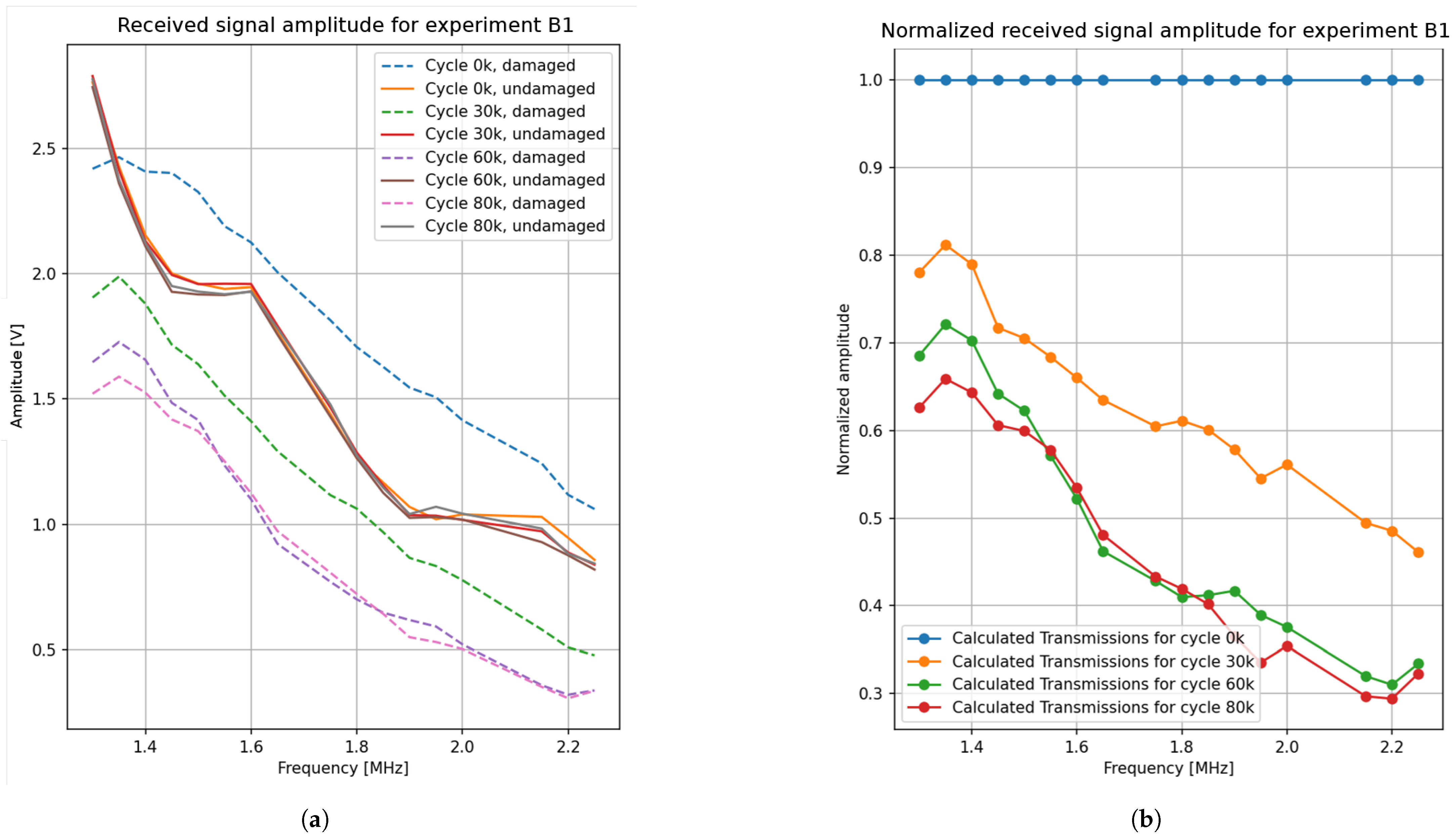
- Amplitude calculation:The maximum amplitudes of the correlations from the previous step are determined, and their square root values are computed. The resulting values from the damaged and undamaged signals correspond to and , respectively. The transmission coefficient is then calculated as the ratio of these two values. This process is repeated for all measurements taken at different excitation frequencies.
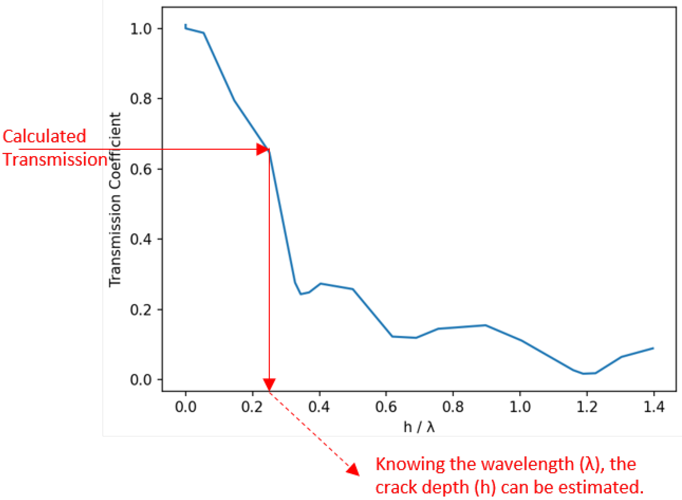
- Transmission coefficient mapping:The transmission coefficients, calculated using formula (1), at various frequencies are analyzed, and outliers are removed. Outliers are defined as transmission coefficients greater than 1 (unrealistic) or lower than 0.35. The latter threshold is based on the transmission graph in Figure 7, which shows that for transmission coefficients below 0.35 there is no monotonic relationship between the coefficient and the crack depth. After filtering, the corresponding crack depth is estimated for each valid transmission coefficient.
- Crack depth estimation:Since a single crack depth is estimated for each excitation frequency in the previous step, a distribution of crack depths is obtained. To remove any remaining outliers, a filtering process using the median absolute deviation (MAD) technique is applied. MAD is a robust statistical measure that calculates the median of the absolute deviations from the dataset’s median:
2.3. Validation Setup
3. Results
3.1. Experimental Data
3.1.1. DI Calculation
3.1.2. Crack Depth Estimation
3.2. Performance Metrics
4. Conclusions
Author Contributions
Funding
Institutional Review Board Statement
Informed Consent Statement
Data Availability Statement
Conflicts of Interest
Abbreviations
| CM | Condition monitoring |
| DI | Damage index |
| ECT | Eddy-current testing |
| EMAT | Electro magnetic acoustic transducers |
| HC | Head checks |
| MAD | Median absolute deviation |
| MFL | Magnetic flux leakag |
| NDT | Non-destructive testing |
| PSU | Piezo switching unit |
| RCF | Rolling contact fatigue |
| RMS | Root mean square |
| SAW | Surface acoustic wave |
| ToF | Time of flight |
| TRV | Track recording vehicles |
| Glossary | |
| CM | condition monitoring. 2 |
| DI | damage index. 8–10, 13, 14, 16 |
| ECT | eddy-current testing. 2 |
| EMAT | electromagnetic acoustic transducer. 2 |
| HC | head check. 1, 13, 15 |
| MAD | median absolute deviation. 13 |
| MFL | magnetic flux leakage. 2 |
| NDT | non-destructive testing. 1, 2 |
| PSU | piezo switching unit. 4, 8, 13, 16 |
| RCF | rolling contact fatigue. 1, 2 |
| RMS | root mean square. 10 |
| SAW | surface acoustic wave. 1–4, 7, 9–11, 16 |
| ToF | time of flight. 9 |
| TRV | track recording vehicle. 1, 11 |
References
- Federal Railroad Administration. Rolling Contact Fatigue: A Comprehensive Review. Technical Report, U.S. Department of Transportation. 2011. Available online: https://railroads.dot.gov/elibrary/rolling-contact-fatigue-comprehensive-review (accessed on 7 May 2025).
- Urassa, P.; Habte, H.S.; Mohammedseid, A. Crack influence and fatigue life assessment in rail profiles: A numerical study. Front. Built Environ. 2023, 9, 1304557. [Google Scholar] [CrossRef]
- Gong, W.; Akbar, M.F.; Jawad, G.N.; Mohamed, M.F.P.; Wahab, M.N.A. Nondestructive Testing Technologies for Rail Inspection: A Review. Coatings 2022, 12, 1790. [Google Scholar] [CrossRef]
- Mićić, M.; Brajović, L.; Lazarević, L.; Popović, Z. Inspection of RCF rail defects—Review of NDT methods. Mech. Syst. Signal Process. 2023, 182, 109568. [Google Scholar] [CrossRef]
- Park, J.W.; Lee, T.G.; Back, I.C.; Seo, J.M.; Kwon, S.G. Rail Surface Defect Detection and Analysis Using Multi-Channel Eddy Current Method Based Algorithm for Defect Evaluation. J. Nondestruct. Eval. 2021, 40, 83. [Google Scholar] [CrossRef]
- Wang, Y.; Wang, Y.; Wang, P.; Ji, K.; Wang, J.; Yang, J.; Shu, Y. Rail Magnetic Flux Leakage Detection and Data Analysis Based on Double-Track Flaw Detection Vehicle. Processes 2023, 11, 1024. [Google Scholar] [CrossRef]
- Tuschl, C.; Oswald-tranta, B.; Eck, S. Inductive thermography as non-destructive testing for railway rails. Appl. Sci. 2021, 11, 1003. [Google Scholar] [CrossRef]
- Tuschl, C.; Oswald-Tranta, B.; Eck, S. Scanning Inductive Thermographic Surface Defect Inspection of Long Flat or Curved Work-Pieces Using Rectification Targets. Appl. Sci. 2022, 12, 5851. [Google Scholar] [CrossRef]
- Tuschl, C.; Oswald-Tranta, B.; Agathocleous, T.; Eck, S. Scanning inductive pulse phase thermography with changing scanning speed for non-destructive testing. Quant. Infrared Thermogr. J. 2024, 21, 156–171. [Google Scholar] [CrossRef]
- Oßberger, U.; Kollment, W.; Eck, S. Insights towards Condition Monitoring of Fixed Railway Crossings. Procedia Struct. Integr. 2017, 4, 106–114. [Google Scholar] [CrossRef]
- Gruber, C.; Hammer, R.; Gänser, H.P.; Künstner, D.; Eck, S. Use of Surface Acoustic Waves for Crack Detection on Railway Track Components—Laboratory Tests. Appl. Sci. 2022, 12, 6334. [Google Scholar] [CrossRef]
- Xue, Z.; Xu, Y.; Hu, M.; Li, S. Systematic review: Ultrasonic technology for detecting rail defects. Constr. Build. Mater. 2023, 368, 130409. [Google Scholar] [CrossRef]
- Swaschnig, P.; Kofler, J.; Klambauer, R.; Bergmann, A. In-line detection of pouch foil damage in batteries during manufacturing using lamb waves. Ndt Int. 2025, 152, 103322. [Google Scholar] [CrossRef]
- Mandal, D.; Bovender, T.; Geil, R.D.; Banerjee, S. Surface Acoustic Waves (SAW) Sensors: Tone-Burst Sensing for Lab-on-a-Chip Devices. Sensors 2024, 24, 644. [Google Scholar] [CrossRef]
- Yu, Y.; Xie, H.; Zhou, T.; Zhang, H.; Lu, C.; Tao, R.; Tang, Z.; Luo, J. Real-Time and Ultrasensitive Prostate-Specific Antigen Sensing Using Love-Mode Surface Acoustic Wave Immunosensor Based on MoS2@Cu2O-Au Nanocomposites. Sensors 2024, 24, 7636. [Google Scholar] [CrossRef]
- Poudel, A.; Lopez, B.; Ali, S.; Bensur, J. In-Motion Railcar Wheel Inspection Using Magnetostrictive EMATs. Mater. Eval. 2024, 82, 42–49. [Google Scholar] [CrossRef]
- Korolev, S.V.; Krasil’nikov, V.A.; Krylo, V.V. Mechanism of sound generation in a solid by a spark discharge near the surface. Sov. Phys. Acoust. 1987, 33, 451–452. [Google Scholar]
- Rezaei, M.; Künstner, D.; Eck, S.; Gänser, H.P. Rail-web mounted pitch-catch piezoelectric setup for detection of head checks using surface acoustic waves. In Proceedings of the Road and Rail Infrastructure VIII: Proceedings of the Conference CETRA 2024, Cavtat, Croatia, 15–17 May 2024; Lakušić, S., Ed.; University of Zagreb Faculty of Civil Engineering: Zagreb, Croatia, 2024; pp. 1037–1045. [Google Scholar] [CrossRef]
- Morichika, S.; Sekiya, H.; Maruyama, O.; Hirano, S.; Miki, C. Fatigue crack detection using a piezoelectric ceramic sensor. Weld World 2020, 64, 141–149. [Google Scholar] [CrossRef]
- Cremins, M.; Shuai, Q.; Xu, J.; Tang, J. Fault detection in railway track using piezoelectric impedance. In Sensors and Smart Structures Technologies for Civil, Mechanical, and Aerospace Systems 2014; Lynch, J.P., Wang, K.W., Sohn, H., Eds.; International Society for Optics and Photonics, SPIE: Bellingham, WA, USA, 2014; Volume 9061. [Google Scholar] [CrossRef]
- Chung, K.J.; Lin, C.W. Condition monitoring for fault diagnosis of railway wheels using recurrence plots and convolutional neural networks (RP-CNN) models. Meas. Control 2024, 57, 330–338. [Google Scholar] [CrossRef]
- Fichtenbauer, S. Towards Continuous Railway Monitoring: A Concept for Surface Crack Assessment Based on Surface Acoustic Waves. Master’s Thesis, Montanuniversitaet Leoben, Leoben, Austria, 2023. [Google Scholar] [CrossRef]
- Stock, R.; Pippan, R. RCF and wear in theory and practice-The influence of rail grade on wear and RCF. Wear 2011, 271, 125–133. [Google Scholar] [CrossRef]
- Mandal, D.; Banerjee, S. Surface Acoustic Wave (SAW) Sensors: Physics, Materials, and Applications. Sensors 2022, 22, 820. [Google Scholar] [CrossRef]
- PI Ceramic GmbH. P-876 DuraAct Patch Transducer. PI Ceramic GmbH, Lederhose, Germany. 2024. Available online: https://www.piceramic.com/en/products/piezoceramic-actuators/patch-transducers/p-876-duraact-patch-transducer-101790 (accessed on 28 April 2025).
- Capineri, L.; Bulletti, A. Ultrasonic Guided-Waves Sensors and Integrated Structural Health Monitoring Systems for Impact Detection and Localization: A Review. Sensors 2021, 21, 2929. [Google Scholar] [CrossRef] [PubMed]
- Hottinger Brüel & Kjaer GmbH. Z70 Cold Curing Superglue. Hottinger Brüel & Kjaer GmbH, Darmstadt, Germany. 2024. Available online: https://www.hbm.com/en/2962/z70-a-single-component-cold-curing-adhesive/ (accessed on 28 April 2025).
- Digilent Inc. Analog Discovery 2: 100MS/s USB Oscilloscope, Logic Analyzer, and Variable Power Supply. 2024. Available online: https://digilent.com/shop/analog-discovery-2-100ms-s-usb-oscilloscope-logic-analyzer-and-variable-power-supply/ (accessed on 28 April 2025).
- Numato Lab. 16-channel relay module—24V, 7A, 240V, 10 GPIO, USB. Available online: https://numato.com/product/16-channel-usb-relay-module/ (accessed on 5 February 2025).
- Yan, J.; Jin, H.; Sun, H.; Qing, X. Active Monitoring of Fatigue Crack in the Weld Zone of Bogie Frames Using Ultrasonic Guided Waves. Sensors 2019, 19, 3372. [Google Scholar] [CrossRef] [PubMed]
- Mariani, S. Non-contact Ultrasonic Guided Wave Inspection of Rails: Next Generation Approach. Ph.D. Thesis, University of California, San Diego, CA, USA, 2015. ProQuest ID: Mariani_ucsd_0033D_14954. Merritt ID: ark:/20775/bb46775949.. [Google Scholar]
- Achenbach, J.; Brind, K.; Keshava, S. Reflection and transmission of obliquely incident Rayleigh waves by a surface-breaking crack. J. Acoust. Soc. Am. 1984, 75, 313–319. [Google Scholar] [CrossRef]
- Leys, C.; Ley, C.; Klein, O.; Bernard, P.; Licata, L. Detecting outliers: Do not use standard deviation around the mean, use the median absolute deviation around the median. J. Exp. Soc. Psychol. 2013, 49, 764–766. [Google Scholar] [CrossRef]


| Specification | P-876.SP1 |
|---|---|
| Dimensions L × W × T (mm) | 16 × 13 × 0.5 |
| Minimum lateral contraction (μm/m) | 650 |
| Relative lateral contraction (μm/m/V) | 1.3 |
| Operating voltage (V) | −100 to 400 |
| Actuator type | Transducer |
| Piezo material | PIC255 |
| Piezoceramic height (μm) | 200 |
| Electrical capacitance (nF) | 8 (±20%) |
| Blocking force (N) | 280 |
| Operating temperature range (°C) | −20 to 150 |
| Connector | Solderable contacts |
| Test Run | Cycle [k] | Estimation Method | Measured Depth [mm] | Estimated Depth [mm] | Error [%] |
|---|---|---|---|---|---|
| B1 | 60 | Proposed algorithm | 0.49 | 0.50 ± 0.019 | +2 |
| B1 | 80 | Proposed algorithm | 0.53 | 0.51 ± 0.032 | −4 |
| B2 | 30 | Proposed algorithm | 0.55 | 0.47 ± 0.077 | −15 |
| B2 | 30 | Eddy current | 0.55 | 0.42 | −24 |
Disclaimer/Publisher’s Note: The statements, opinions and data contained in all publications are solely those of the individual author(s) and contributor(s) and not of MDPI and/or the editor(s). MDPI and/or the editor(s) disclaim responsibility for any injury to people or property resulting from any ideas, methods, instructions or products referred to in the content. |
© 2025 by the authors. Licensee MDPI, Basel, Switzerland. This article is an open access article distributed under the terms and conditions of the Creative Commons Attribution (CC BY) license (https://creativecommons.org/licenses/by/4.0/).
Share and Cite
Rezaei, M.; Eck, S.; Fichtenbauer, S.; Maierhofer, J.; Klambauer, R.; Bergmann, A.; Künstner, D.; Velic, D.; Gänser, H.-P. Real-Time Detection and Quantification of Rail Surface Cracks Using Surface Acoustic Waves and Piezoelectric Patch Transducers. Sensors 2025, 25, 3014. https://doi.org/10.3390/s25103014
Rezaei M, Eck S, Fichtenbauer S, Maierhofer J, Klambauer R, Bergmann A, Künstner D, Velic D, Gänser H-P. Real-Time Detection and Quantification of Rail Surface Cracks Using Surface Acoustic Waves and Piezoelectric Patch Transducers. Sensors. 2025; 25(10):3014. https://doi.org/10.3390/s25103014
Chicago/Turabian StyleRezaei, Mohsen, Sven Eck, Sebastian Fichtenbauer, Jürgen Maierhofer, Reinhard Klambauer, Alexander Bergmann, David Künstner, Dino Velic, and Hans-Peter Gänser. 2025. "Real-Time Detection and Quantification of Rail Surface Cracks Using Surface Acoustic Waves and Piezoelectric Patch Transducers" Sensors 25, no. 10: 3014. https://doi.org/10.3390/s25103014
APA StyleRezaei, M., Eck, S., Fichtenbauer, S., Maierhofer, J., Klambauer, R., Bergmann, A., Künstner, D., Velic, D., & Gänser, H.-P. (2025). Real-Time Detection and Quantification of Rail Surface Cracks Using Surface Acoustic Waves and Piezoelectric Patch Transducers. Sensors, 25(10), 3014. https://doi.org/10.3390/s25103014