
Early Prediction of Sepsis Onset Using Neural Architecture Search Based on Genetic Algorithms


Abstract
:1. Introduction
2. Methods
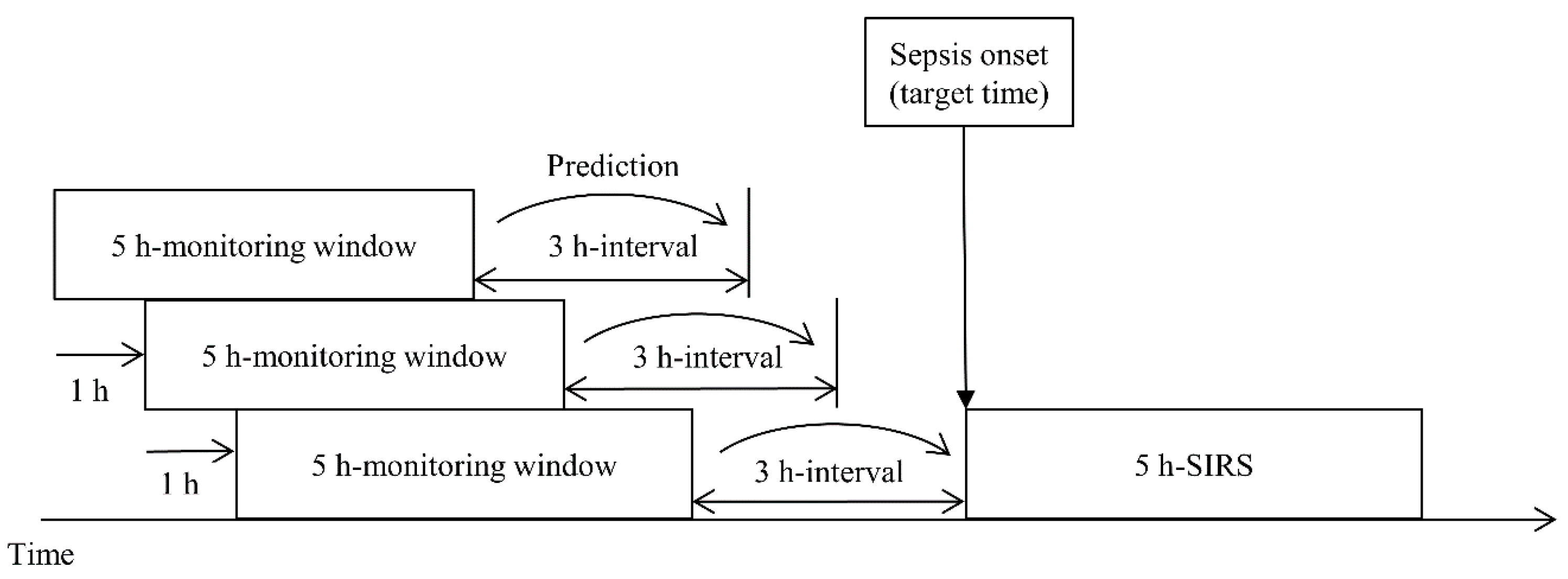
2.1. Gold Standard
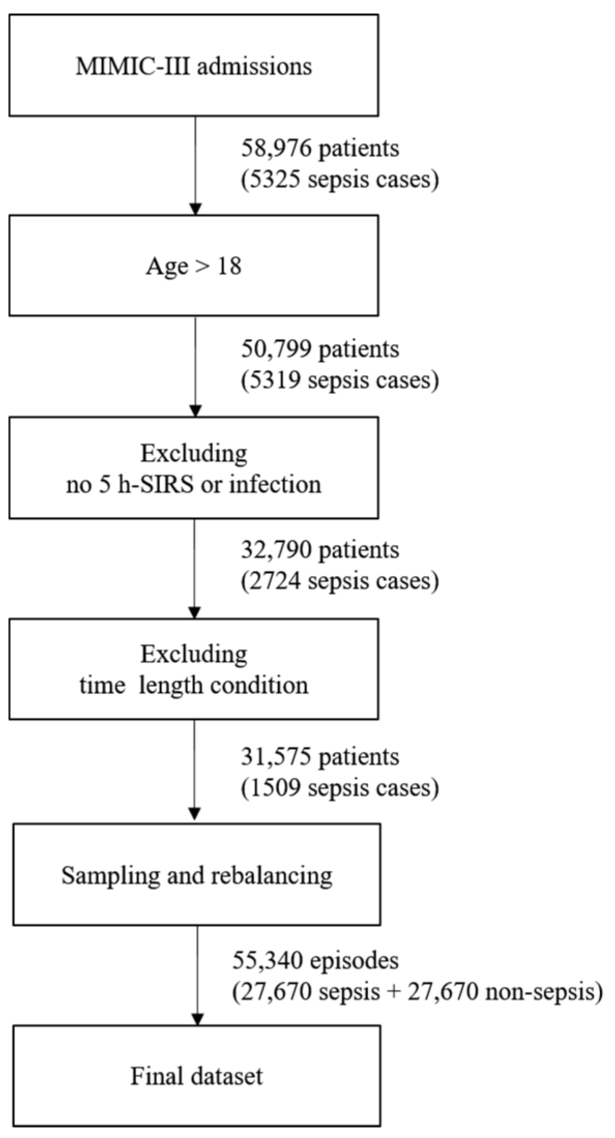
2.2. Dataset
2.3. Feature Extraction
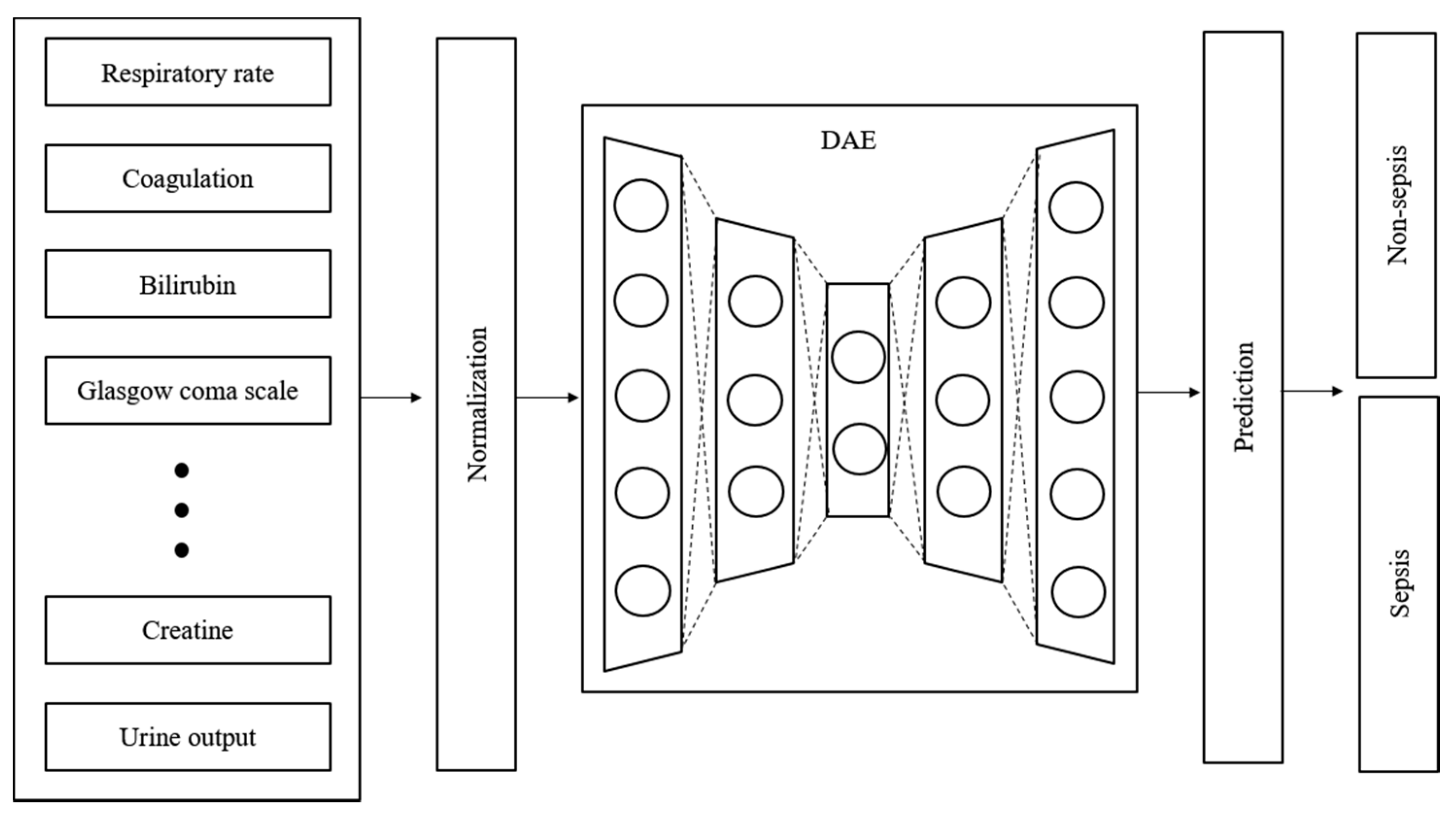
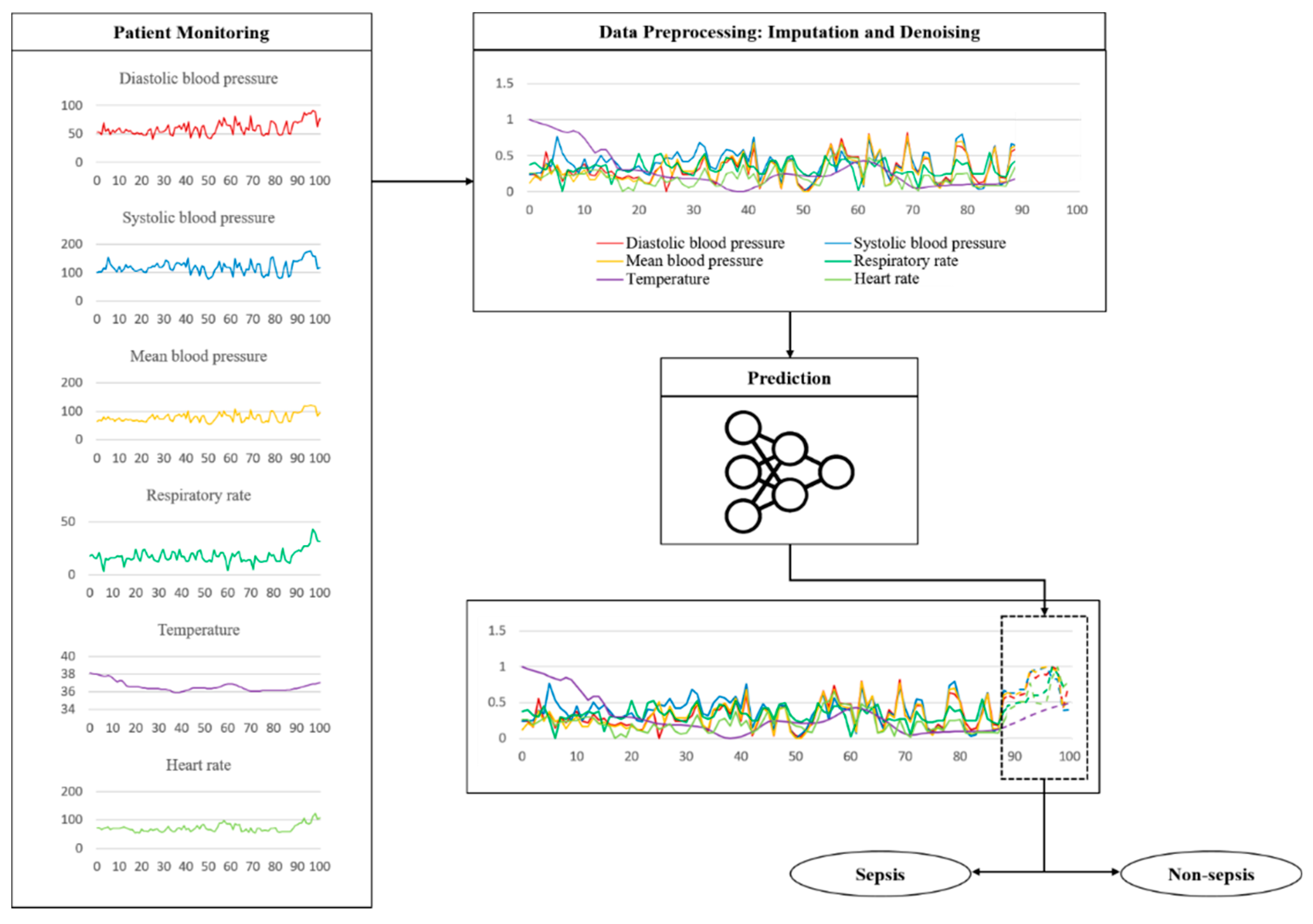
2.4. Imputation and Denoising
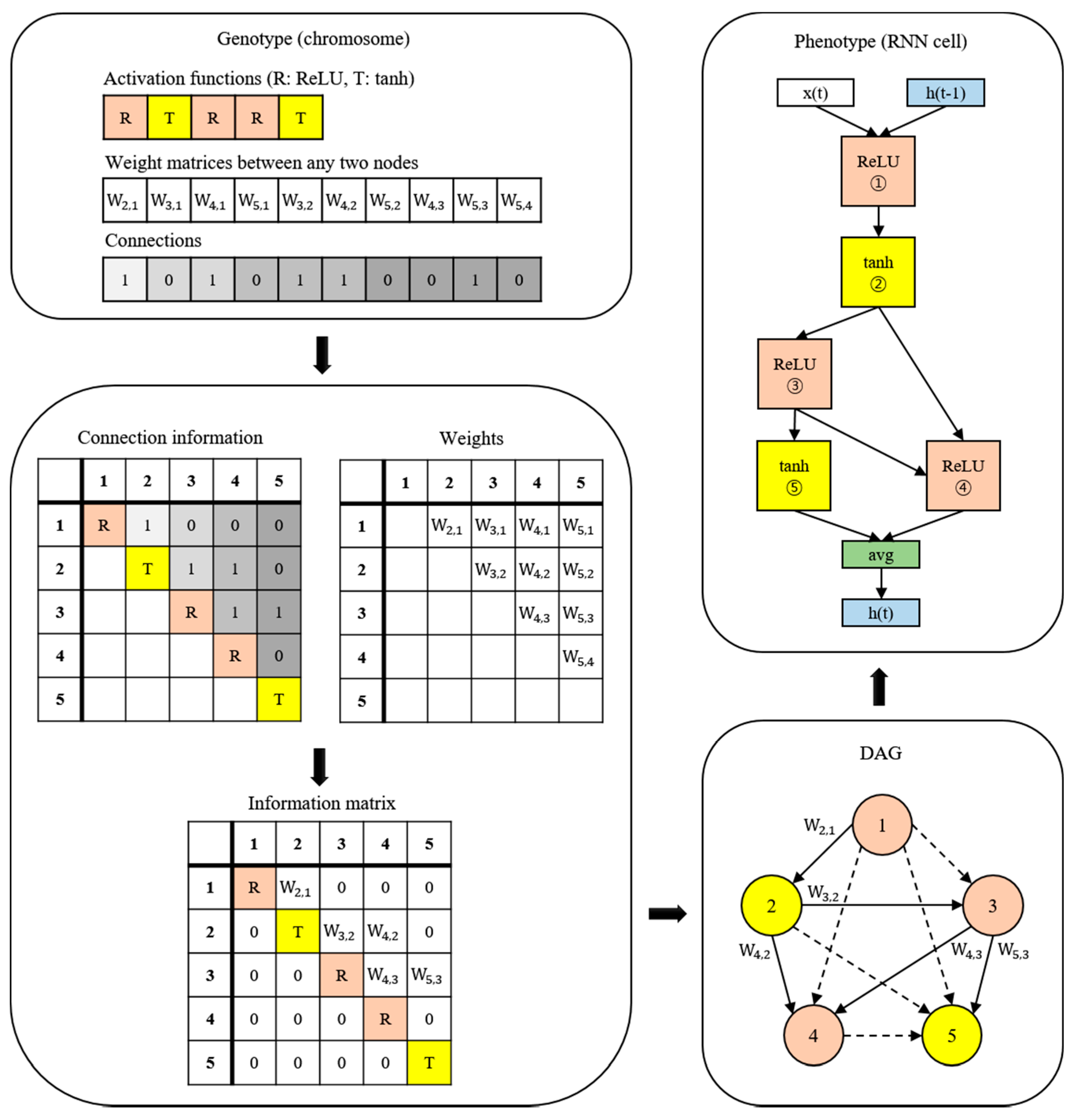
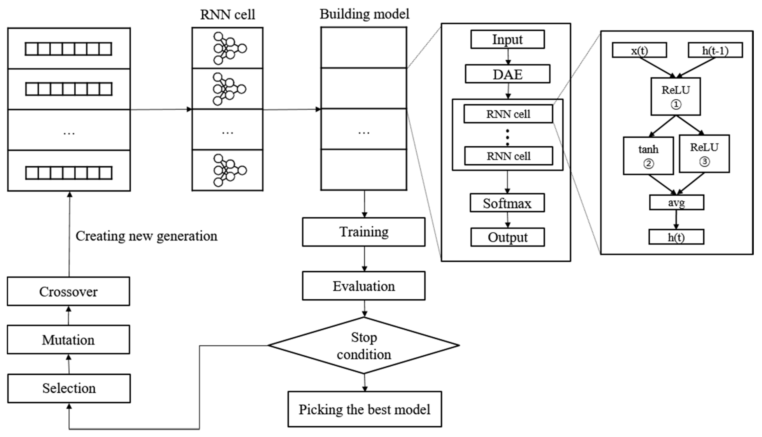
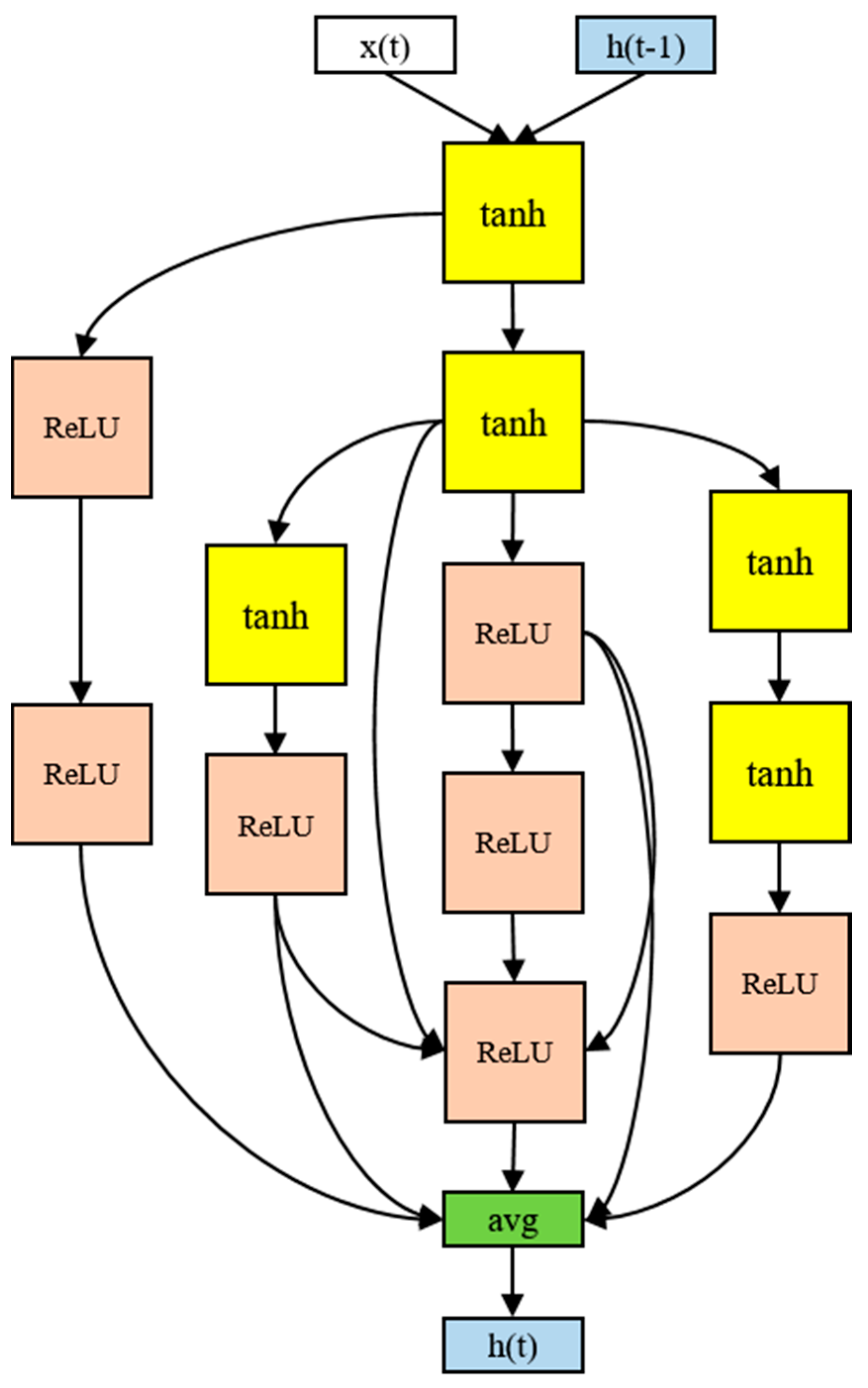
2.5. Proposed Model
2.6. Evaluation
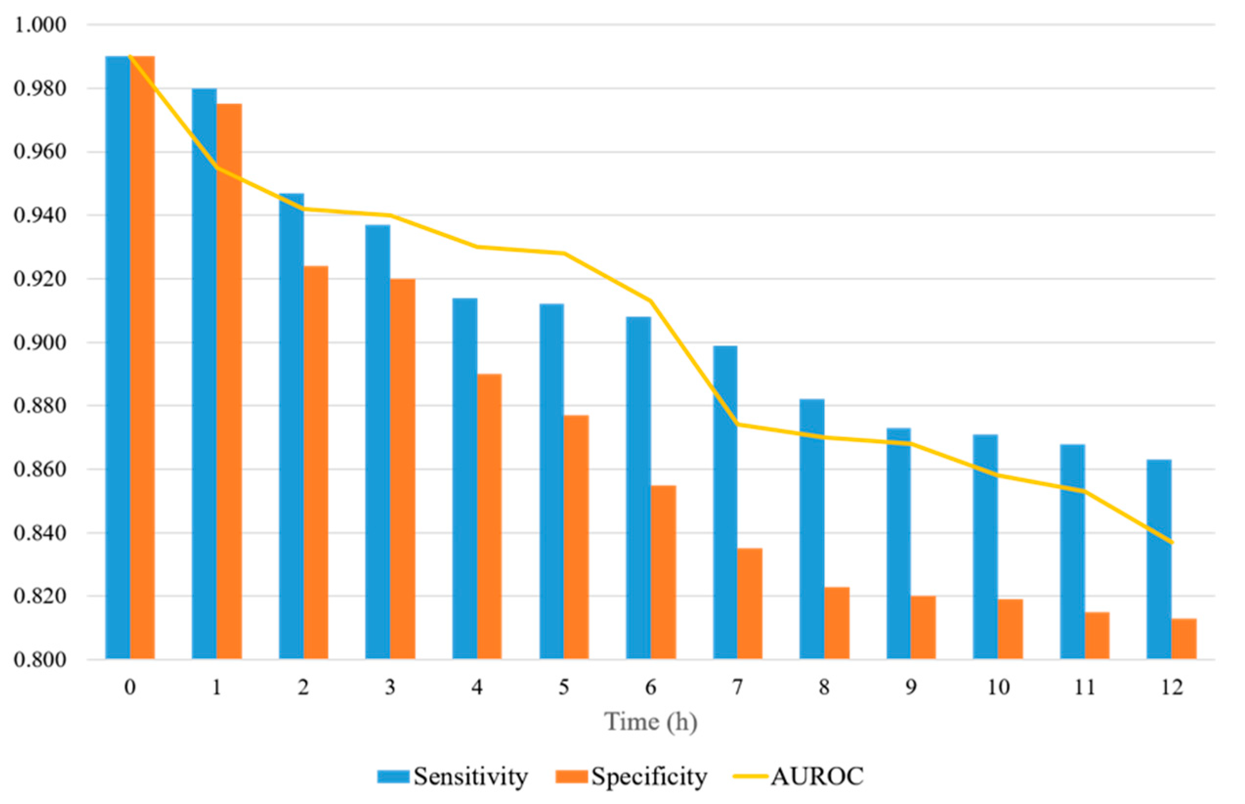
3. Results
4. Discussion
5. Conclusions
Author Contributions
Funding
Institutional Review Board Statement
Informed Consent Statement
Data Availability Statement
Conflicts of Interest
References
- Singer, M.; Deutschman, C.S.; Seymour, C.W.; Shankar-Hari, M.; Annane, D.; Bauer, M.; Bellomo, R.; Bernard, G.R.; Chiche, J.-D.; Coopersmith, C.M.; et al. The Third International Consensus Definitions for Sepsis and Septic Shock (Sepsis-3). JAMA 2016, 315, 801–810. [Google Scholar] [CrossRef]
- Reyna, M.A.; Josef, C.S.; Jeter, R.; Shashikumar, S.P.; Westover, M.B.; Nemati, S.; Clifford, G.D.; Sharma, A. Early Prediction of Sepsis from Clinical Data: The PhysioNet/Computing in Cardiology Challenge 2019. Crit. Care Med. 2020, 48, 210–217. [Google Scholar] [CrossRef] [Green Version]
- Giamarellos-Bourboulis, E.J.; Tsaganos, T.; Tsangaris, I.; Lada, M.; Routsi, C.; Sinapidis, D.; Koupetori, M.; Bristianou, M.; Adamis, G.; Mandragos, K.; et al. Validation of the New Sepsis-3 Definitions: Proposal for Improvement in Early Risk Identification. Clin. Microbiol. Infect. 2017, 23, 104–109. [Google Scholar] [CrossRef] [PubMed] [Green Version]
- Dykes, L.A.; Heintz, S.J.; Heintz, B.H.; Livorsi, D.J.; Egge, J.A.; Lund, B.C. Contrasting QSOFA and SIRS Criteria for Early Sepsis Identification in a Veteran Population. Fed. Pract. 2019, 36, S21–S24. [Google Scholar]
- Bone, R.C.; Balk, R.A.; Cerra, F.B.; Dellinger, R.P.; Fein, A.M.; Knaus, W.A.; Schein, R.M.H.; Sibbald, W.J. Definitions for Sepsis and Organ Failure and Guidelines for the Use of Innovative Therapies in Sepsis. Chest 1992, 101, 1644–1655. [Google Scholar] [CrossRef] [PubMed] [Green Version]
- Song, J.-U.; Sin, C.K.; Park, H.K.; Shim, S.R.; Lee, J. Performance of the Quick Sequential (Sepsis-Related) Organ Failure Assessment Score as a Prognostic Tool in Infected Patients Outside the Intensive Care Unit: A Systematic Review and Meta-Analysis. Crit. Care 2018, 22, 28. [Google Scholar] [CrossRef] [PubMed] [Green Version]
- Kim, Y.H.; Yeo, J.H.; Kang, M.J.; Lee, J.H.; Cho, K.W.; Hwang, S.; Hong, C.K.; Lee, Y.H.; Kim, Y.W. Performance Assessment of the SOFA, APACHE II Scoring System, and SAPS II in Intensive Care Unit Organophosphate Poisoned Patients. J. Korean Med. Sci. 2013, 28, 1822. [Google Scholar] [CrossRef] [PubMed] [Green Version]
- Huang, J.; Xuan, D.; Li, X.; Ma, L.; Zhou, Y.; Zou, H. The Value of APACHE II in Predicting Mortality after Paraquat Poisoning in Chinese and Korean Population: A Systematic Review and Meta-Analysis. Medicine (Baltimore) 2017, 96, e6838. [Google Scholar] [CrossRef]
- Le Gall, J.; Neumann, A.; Hemery, F.; Bleriot, J.; Fulgencio, J.; Garrigues, B.; Gouzes, C.; Lepage, E.; Moine, P.; Villers, D. Mortality Prediction Using SAPS II: An Update for French Intensive Care Units. Crit. Care 2005, 9, R645. [Google Scholar] [CrossRef] [PubMed] [Green Version]
- Gao, X.W.; Hui, R.; Tian, Z. Classification of CT Brain Images Based on Deep Learning Networks. Comput. Methods Programs Biomed. 2017, 138, 49–56. [Google Scholar] [CrossRef] [Green Version]
- Li, W.; Jia, F.; Hu, Q. Automatic Segmentation of Liver Tumor in CT Images with Deep Convolutional Neural Networks. J. Comput. Commun. 2015, 03, 146–151. [Google Scholar] [CrossRef] [Green Version]
- Gherardini, M.; Mazomenos, E.; Menciassi, A.; Stoyanov, D. Catheter Segmentation in X-Ray Fluoroscopy Using Synthetic Data and Transfer Learning with Light U-Nets. Comput. Methods Programs Biomed. 2020, 192, 105420. [Google Scholar] [CrossRef]
- Islam, M.M.; Nasrin, T.; Walther, B.A.; Wu, C.-C.; Yang, H.-C.; Li, Y.-C. Prediction of Sepsis Patients Using Machine Learning Approach: A Meta-Analysis. Comput. Methods Programs Biomed. 2019, 170, 1–9. [Google Scholar] [CrossRef]
- Scherpf, M.; Gräßer, F.; Malberg, H.; Zaunseder, S. Predicting Sepsis with a Recurrent Neural Network Using the MIMIC III Database. Comput. Biol. Med. 2019, 113, 103395. [Google Scholar] [CrossRef] [PubMed]
- Zhang, Y.; Lin, C.; Chi, M.; Ivy, J.; Capan, M.; Huddleston, J.M. LSTM for Septic Shock: Adding Unreliable Labels to Reliable Predictions. In Proceedings of the 2017 IEEE International Conference on Big Data (Big Data), Boston, MA, USA, 11–14 December 2017; pp. 1233–1242. [Google Scholar]
- Saqib, M.; Sha, Y.; Wang, M.D. Early Prediction of Sepsis in EMR Records Using Traditional ML Techniques and Deep Learning LSTM Networks. In Proceedings of the 2018 40th Annual International Conference of the IEEE Engineering in Medicine and Biology Society (EMBC), Honolulu, HI, USA, 18–21 July 2018; pp. 4038–4041. [Google Scholar]
- Oh, S.L.; Ng, E.Y.K.; Tan, R.S.; Acharya, U.R. Automated Diagnosis of Arrhythmia Using Combination of CNN and LSTM Techniques with Variable Length Heart Beats. Comput. Biol. Med. 2018, 102, 278–287. [Google Scholar] [CrossRef]
- Zhang, J.; Sun, Y.; Guo, L.; Gao, H.; Hong, X.; Song, H. A New Bearing Fault Diagnosis Method Based on Modified Convolutional Neural Networks. Chin. J. Aeronaut. 2020, 33, 439–447. [Google Scholar] [CrossRef]
- Fagerström, J.; Bång, M.; Wilhelms, D.; Chew, M.S. LiSep LSTM: A Machine Learning Algorithm for Early Detection of Septic Shock. Sci. Rep. 2019, 9, 15132. [Google Scholar] [CrossRef] [Green Version]
- Kam, H.J.; Kim, H.Y. Learning Representations for the Early Detection of Sepsis with Deep Neural Networks. Comput. Biol. Med. 2017, 89, 248–255. [Google Scholar] [CrossRef]
- Elsken, T.; Metzen, J.H.; Hutter, F. Neural Architecture Search: A Survey. J. Mach. Learn. Res. 2019, 20, 1997–2017. [Google Scholar]
- Pham, H.; Guan, M.Y.; Zoph, B.; Le, Q.V.; Dean, J. Efficient Neural Architecture Search via Parameter Sharing. In Proceedings of the 35th International Conference on Machine Learning, Stockholm, Sweden, 10–15 July 2018; pp. 4095–4104. [Google Scholar]
- Chen, Y.; Meng, G.; Zhang, Q.; Xiang, S.; Huang, C.; Mu, L.; Wang, X. RENAS: Reinforced Evolutionary Neural Architecture Search. In Proceedings of the 2019 IEEE/CVF Conference on Computer Vision and Pattern Recognition (CVPR), Long Beach, CA, USA, 15–20 June 2019; pp. 4782–4791. [Google Scholar]
- Calvert, J.S.; Price, D.A.; Chettipally, U.K.; Barton, C.W.; Feldman, M.D.; Hoffman, J.L.; Jay, M.; Das, R. A Computational Approach to Early Sepsis Detection. Comput. Biol. Med. 2016, 74, 69–73. [Google Scholar] [CrossRef] [Green Version]
- Johnson, A.E.W.; Pollard, T.J.; Shen, L.; Lehman, L.H.; Feng, M.; Ghassemi, M.; Moody, B.; Szolovits, P.; Anthony Celi, L.; Mark, R.G. MIMIC-III, a Freely Accessible Critical Care Database. Sci. Data 2016, 3, 160035. [Google Scholar] [CrossRef] [Green Version]
- Gui, Q.; Jin, Z.; Xu, W. Exploring Missing Data Prediction in Medical Monitoring: A Performance Analysis Approach. In Proceedings of the 2014 IEEE Signal Processing in Medicine and Biology Symposium (SPMB), Philadelphia, PA, USA, 13 December 2014; pp. 1–6. [Google Scholar]
- Liu, P.; Zheng, P.; Chen, Z. Deep Learning with Stacked Denoising Auto-Encoder for Short-Term Electric Load Forecasting. Energies 2019, 12, 2445. [Google Scholar] [CrossRef] [Green Version]
- Vincent, P.; Larochelle, H.; Lajoie, I.; Bengio, Y.; Manzagol, P.-A. Stacked Denoising Autoencoders: Learning Useful Representations in a Deep Network with a Local Denoising Criterion. J. Mach. Learn. Res. 2010, 11, 3371–3408. [Google Scholar]
- Holland, J.H. Genetic Algorithms and Adaptation. In Adaptive Control of Ill-Defined Systems; Selfridge, O.G., Rissland, E.L., Arbib, M.A., Eds.; Springer: Boston, MA, USA, 1984; pp. 317–333. ISBN 978-1-4684-8943-9. [Google Scholar]
- Desautels, T.; Calvert, J.; Hoffman, J.; Jay, M.; Kerem, Y.; Shieh, L.; Shimabukuro, D.; Chettipally, U.; Feldman, M.D.; Barton, C.; et al. Prediction of Sepsis in the Intensive Care Unit With Minimal Electronic Health Record Data: A Machine Learning Approach. JMIR Med. Inform. 2016, 4, e5909. [Google Scholar] [CrossRef]
- Nemati, S.; Holder, A.; Razmi, F.; Stanley, M.D.; Clifford, G.D.; Buchman, T.G. An Interpretable Machine Learning Model for Accurate Prediction of Sepsis in the ICU. Crit. Care Med. 2018, 46, 547–553. [Google Scholar] [CrossRef] [PubMed]
- Khojandi, A.; Tansakul, V.; Li, X.; Koszalinski, R.S.; Paiva, W. Prediction of Sepsis and In-Hospital Mortality Using Electronic Health Records. Methods Inf. Med. 2018, 57, 185–193. [Google Scholar] [CrossRef]
- Moor, M.; Horn, M.; Rieck, B.; Roqueiro, D.; Borgwardt, K. Early Recognition of Sepsis with Gaussian Process Temporal Convolutional Networks and Dynamic Time Warping. In Proceedings of the 4th Machine Learning for Healthcare Conference, Ann Arbor, MI, USA, 8–10 August 2019; pp. 2–26. [Google Scholar]
- Li, X.; Ng, G.A.; Schlindwein, F.S. Convolutional and Recurrent Neural Networks for Early Detection of Sepsis Using Hourly Physiological Data from Patients in Intensive Care Unit. In Proceedings of the 2019 Computing in Cardiology (CinC), Singapore, 8–11 September 2019; pp. 1–4. [Google Scholar]
- Lauritsen, S.M.; Kalør, M.E.; Kongsgaard, E.L.; Lauritsen, K.M.; Jørgensen, M.J.; Lange, J.; Thiesson, B. Early Detection of Sepsis Utilizing Deep Learning on Electronic Health Record Event Sequences. Artif. Intell. Med. 2020, 104, 101820. [Google Scholar] [CrossRef]
- Yang, M.; Liu, C.; Wang, X.; Li, Y.; Gao, H.; Liu, X.; Li, J. An Explainable Artificial Intelligence Predictor for Early Detection of Sepsis. Crit. Care Med. 2020, 48, e1091–e1096. [Google Scholar] [CrossRef] [PubMed]
- Bedoya, A.D.; Futoma, J.; Clement, M.E.; Corey, K.; Brajer, N.; Lin, A.; Simons, M.G.; Gao, M.; Nichols, M.; Balu, S.; et al. Machine Learning for Early Detection of Sepsis: An Internal and Temporal Validation Study. JAMIA Open 2020, 3, 252–260. [Google Scholar] [CrossRef]
- Li, Q.; Li, L.; Zhong, J.; Huang, L.F. Real-Time Sepsis Severity Prediction on Knowledge Graph Deep Learning Networks for the Intensive Care Unit. J. Vis. Commun. Image Represent. 2020, 72, 102901. [Google Scholar] [CrossRef]
- Shashikumar, S.P.; Josef, C.S.; Sharma, A.; Nemati, S. DeepAISE—An Interpretable and Recurrent Neural Survival Model for Early Prediction of Sepsis. Artif. Intell. Med. 2021, 113, 102036. [Google Scholar] [CrossRef] [PubMed]
- Rafiei, A.; Rezaee, A.; Hajati, F.; Gheisari, S.; Golzan, M. SSP: Early Prediction of Sepsis Using Fully Connected LSTM-CNN Model. Comput. Biol. Med. 2021, 128, 104110. [Google Scholar] [CrossRef] [PubMed]
- Li, H.; Xu, Z.; Taylor, G.; Studer, C.; Goldstein, T. Visualizing the Loss Landscape of Neural Nets. In Proceedings of the 32nd International Conference on Neural Information Processing Systems, Montréal, QC, Canada, 3–8 December 2018; pp. 6391–6401. [Google Scholar]


| Overall | |
|---|---|
| Admission | 58,976 |
| Adult patients | 38,425 |
| Age | 65.86 (52.72–77.97) |
| Gender (female) | 15,409 |
| HR 1 (bpm) | 84.00 (73.00–97.00) |
| MAP 2 (mmHg) | 76.00 (67.33–87.00) |
| RR 3 (cpm) | 18.00 (14.00–22.00) |
| Na (mmol/L) | 138.00 (136.00–141.00) |
| K (mmol/L) | 4.10 (3.80–4.60) |
| HCO3 (mmol/L) | 24.00 (21.00–26.00) |
| WBC 4 (×103/mm3) | 11.00 (7.90–14.90) |
| PaO2/FiO2 ratio | 267.50 (180.00–352.50) |
| Ht 5 (%) | 31.00 (26.00–36.00) |
| Urea (mmol/L) | 1577.00 (968.00–2415.00) |
| Bilirubin (mg/dL) | 0.7 (0.40–1.70) |
| Feature | ID | Name |
|---|---|---|
| Heart rate | 211 | Heart Rate |
| 220045 | Heart Rate | |
| Temperature | 678 | Temperature F |
| 223761 | Temperature Fahrenheit | |
| 676 | Temperature C | |
| 223762 | Temperature Celsius | |
| Systolic blood pressure | 51 | Arterial BP (Systolic) |
| 442 | Manual BP (Systolic) | |
| 455 | NBP (Systolic) | |
| 6701 | Arterial BP #2 (Systolic) | |
| 220179 | Non-Invasive Blood Pressure systolic | |
| 220050 | Arterial Blood Pressure systolic | |
| PaO2/FiO2 ratio | 50821 | PO2 |
| 50816 | Oxygen | |
| 223835 | Inspired O2 Fraction | |
| 3420 | FiO2 | |
| 3422 | FiO2 (Meas) | |
| 190 | FiO2 Set | |
| White blood cells count | 51300 | WBC Count |
| 51301 | White Blood Cells | |
| Glasgow coma scale | 723 | Verbal Response |
| 454 | Motor Response | |
| 184 | Eye Opening | |
| 223900 | GCS—Verbal Response | |
| 223901 | GCS—Motor Response | |
| 220739 | GCS—Eye Opening |
| SOFA | qSOFA | SAPS II | InSight | |
|---|---|---|---|---|
| Age | O | O | ||
| Heart rate | O | O | ||
| pH | O | |||
| Systolic blood pressure | O | O | O | |
| Pulse pressure | O | |||
| Temperature | O | O | ||
| Respiratory rate | O | |||
| Glasgow coma scale | O | O | O | |
| Mechanical ventilation or CPAP | O | |||
| PaO2 | O | O | O | |
| FiO2 | O | O | O | |
| Urine output | O | O | ||
| Blood urea nitrogen | O | |||
| Blood oxygen saturation | O | |||
| Sodium | O | |||
| Potassium | O | |||
| Bicarbonate | O | |||
| Bilirubin | O | O | ||
| White blood cell count | O | O | ||
| Chronic diseases | O | |||
| Type of admission | O | |||
| Platelets | O | |||
| Creatinine | O | |||
| Mean arterial pressure | O | |||
| Dopamine | O | |||
| Epinephrine | O | |||
| Norepinephrine | O |
| Authors | Dataset | Model | Prediction Time | Sensitivity | Specificity | AUROC (95% CI) |
|---|---|---|---|---|---|---|
| Calvert et al. [24], 2016 | MIMIC-II | InSight | 3 h | 0.90 | 0.81 | 0.83 |
| Desautels et al. [30], 2016 | MIMIC-III | InSight | 4 h | 0.80 | 0.54 | 0.74 |
| Kam et al. [20], 2017 | MIMIC-II | LSTM | 3 h | 0.91 | 0.94 | 0.93 |
| Nemati et al. [31], 2018 | MIMIC-III | AISE | 4 h | 0.85 | 0.67 | 0.85 |
| Khojandi et al. [32], 2018 | Oklahoma State University | RF | 0 h | 0.99 | 0.97 | 0.90 |
| Moor et al. [33], 2019 | MIMIC-III | MGP-TCN | 7 h | - | - | 0.86 |
| Li et al. [34], 2019 | 2019 PhysioNet/CinC Challenge dataset | CNN+RNN | 12 h | - | - | 0.75 |
| Scherpf et al. [14], 2019 | MIMIC-III | RNN | 3 h | 0.90 | 0.47 | 0.81 (0.79–0.83) |
| Lauritsen et al. [35], 2020 | The Danish National Patient Registry | CNN+LSTM | 3 h | - | - | 0.86 |
| Yang et al. [36], 2020 | 2019 PhysioNet/CinC Challenge dataset | XGBOOST | 1 h | 0.90 | 0.64 | 0.85 |
| Bedoya et al. [37], 2020 | Duke University Hospital | MGP-RNN | 4 h | - | - | 0.88 (0.87–0.89) |
| Li et al. [38], 2020 | 2019 PhysioNet/CinC Challenge dataset | LightGBM | 6 h | 0.86 | 0.63 | 0.85 |
| Shashikumar et al. [39], 2021 | MIMIC-III | DeepAISE | 4 h | 0.80 | 0.75 | 0.87 |
| Rafiei et al. [40], 2021 | 2019 PhysioNet/CinC Challenge dataset | SSP | 4 h | 0.85 | 0.81 | 0.92 |
| This study | MIMIC-III | SOFA | 3 h | 0.65 | 0.58 | 0.63 (0.59–0.67) |
| qSOFA | 3 h | 0.61 | 0.75 | 0.65 (0.62–0.68) | ||
| SAPS II | 3 h | 0.65 | 0.77 | 0.68 (0.66–0.70) | ||
| LSTM | 3 h | 0.83 | 0.74 | 0.84 (0.81–0.87) | ||
| The proposed model | 3 h | 0.93 | 0.91 | 0.94 (0.92–0.96) | ||
| 4 h | 0.91 | 0.86 | 0.93 (0.92–0.94) | |||
| 8 h | 0.88 | 0.82 | 0.87 (0.84–0.90) | |||
| 12 h | 0.86 | 0.81 | 0.83 (0.81–0.85) |
Publisher’s Note: MDPI stays neutral with regard to jurisdictional claims in published maps and institutional affiliations. |
© 2022 by the authors. Licensee MDPI, Basel, Switzerland. This article is an open access article distributed under the terms and conditions of the Creative Commons Attribution (CC BY) license (https://creativecommons.org/licenses/by/4.0/).
Share and Cite
Kim, J.K.; Ahn, W.; Park, S.; Lee, S.-H.; Kim, L. Early Prediction of Sepsis Onset Using Neural Architecture Search Based on Genetic Algorithms. Int. J. Environ. Res. Public Health 2022, 19, 2349. https://doi.org/10.3390/ijerph19042349
Kim JK, Ahn W, Park S, Lee S-H, Kim L. Early Prediction of Sepsis Onset Using Neural Architecture Search Based on Genetic Algorithms. International Journal of Environmental Research and Public Health. 2022; 19(4):2349. https://doi.org/10.3390/ijerph19042349
Chicago/Turabian StyleKim, Jae Kwan, Wonbin Ahn, Sangin Park, Soo-Hong Lee, and Laehyun Kim. 2022. "Early Prediction of Sepsis Onset Using Neural Architecture Search Based on Genetic Algorithms" International Journal of Environmental Research and Public Health 19, no. 4: 2349. https://doi.org/10.3390/ijerph19042349
APA StyleKim, J. K., Ahn, W., Park, S., Lee, S.-H., & Kim, L. (2022). Early Prediction of Sepsis Onset Using Neural Architecture Search Based on Genetic Algorithms. International Journal of Environmental Research and Public Health, 19(4), 2349. https://doi.org/10.3390/ijerph19042349